Article

A Lookahead Behavior Model for Multi-Agent Hybrid Simulation

College of Information System and Management, National University of Defense Technology, Changsha 410073, Hunan, China
*
Author to whom correspondence should be addressed.
Appl. Sci. 2017, 7(10), 1095; https://doi.org/10.3390/app7101095
Submission received: 28 August 2017 / Revised: 17 October 2017 / Accepted: 18 October 2017 / Published: 24 October 2017
(This article belongs to the Special Issue Modeling, Simulation, Operation and Control of Discrete Event Systems)

Abstract

:
In the military field, multi-agent simulation (MAS) plays an important role in studying wars statistically. For a military simulation system, which involves large-scale entities and generates a very large number of interactions during the runtime, the issue of how to improve the running efficiency is of great concern for researchers. Current solutions mainly use hybrid simulation to gain fewer updates and synchronizations, where some important continuous models are maintained implicitly to keep the system dynamics, and partial resynchronization (PR) is chosen as the preferable state update mechanism. However, problems, such as resynchronization interval selection and cyclic dependency, remain unsolved in PR, which easily lead to low update efficiency and infinite looping of the state update process. To address these problems, this paper proposes a lookahead behavior model (LBM) to implement a PR-based hybrid simulation. In LBM, a minimal safe time window is used to predict the interactions between implicit models, upon which the resynchronization interval can be efficiently determined. Moreover, the LBM gives an estimated state value in the lookahead process so as to break the state-dependent cycle. The simulation results show that, compared with traditional mechanisms, LBM requires fewer updates and synchronizations.

1. Introduction

Agent-based modeling and simulation has become the primary means of studying complex adaptive systems (CAS). It constructs the basic elements in the system as agents. Through the agents and interactions among them, it generates system changes and, therefore, forms a bottom-up perspective for people to simulate and research the emergent behavior of the system, where the nature of the system can be understood much better. The behavior model of a typical agent can be built using a generic “sense-think-act” paradigm [1,2,3,4] in multi-agent simulation (MAS). The steps in this paradigm include the agent’s process of perceiving the environment, making decisions, and acting, which correspond to the sense-think-act cycle, respectively.
MAS can be applied not only to predict the behaviors of simple systems under specific conditions, but also to research the statistical trends in complex systems [5,6,7,8,9,10,11]. A number of typical applications in this work include disaster emergency management [12], traffic management [13,14], military online decision-making [15,16], and so on. These applications adjust the uncertain parameters by a set of stochastic numbers to obtain a large sample space for iterative calculations [17], so as to evaluate various plans and finally obtain several near-optimal solutions for decision-makers.
However, in the simulation of complex systems, the typical time-stepped sense-think-act cycle takes a great deal more time when agents—and thus their interactions—are enormous. For example, the computing efficiency of MANA (map-aware non-uniform automata) system [18] for combat operations, when the number of agents reaches 600, will be greatly reduced [19]. In military applications, the system usually consists of a large number of autonomous or semi-autonomous combat units, which require large-scale agents. This large-scale simulation, even in one iteration, would consume a great deal of time, rendering the time needed for optimal planning selection unable to be reasonably controlled. Therefore, the efficiency of the MAS becomes the vital aspect to be considered in a large-scale complex simulation system, especially in simulation-based optimization applications.
A common approach proposed to improve the computational efficiency is hybrid agent-based simulation, which introduces discrete event simulation (DES) into agent-based models [20,21,22,23]. As the discrete event-based approach does not need to scan the simulation model continuously when the system state stays unchanged, it is generally believed that the efficiency of the scheduling strategy based on discrete events is higher than that of the time-stepped method of periodic scanning [24].
It has been found that MAS and DES become a pair of contradictions for continuous models in the ways of state updating and the predictability of the agent behavior [25,26,27]. Complex systems in the real world are mixtures of continuous and discrete systems [28,29]. There is often a need to retain the continuity of the object characteristics so as to capture the system dynamics. Thus, the time-stepped simulation is much more applicable in most typical MAS.
Therefore, the matter of how to update the agent state is the main focus in building a hybrid simulation. According to its ways of implementation, the state update mechanism can be divided into fixed time synchronization (FS), variable time synchronization (VS), optimistic synchronization (OS), complete resynchronization (CR), and partial resynchronization (PR), which will be discussed in detail in Section 2. Among them, PR is an outstanding method in hybrid simulation with fewer updates and sync numbers. As shown in Reference [20], the PR method can greatly improve the computational efficiency in the National Airspace System when the agent requires frequent interaction and the state update time changes considerably.
However, there are still problems that need to be addressed when developing PR-based simulations, two of which are the resynchronization interval (RI) and cyclic dependency (CD). Smaller RI brings more re-sync times, while larger RI may result in missing important interactions. CD causes an infinite loop in the synchronization of states.
Aiming at tackling these two problems, this paper proposes a lookahead behavior model (LBM) for hybrid simulation. LBM uses a time window-based lookahead process to implement hybrid simulations under the PR mechanism. The goal of the method is to create a nearest next “safe” time window when advancing simulation time. On one hand, the interaction events that will happen in relation to two agents can be predicted in the time window, to determine when a resynchronization is needed between them. On the other hand, estimated values are introduced in a time window for an agent in the cyclic dependency so as to break the loop occurring in the state synchronization. This paper describes the lookahead modeling process in a simple military test case and compares the efficiency of the PR mechanism with those of other state update mechanisms. The results show that, compared to traditional agent behavior models (TBMs) with fixed time synchronization or variable time synchronization, LBM allows simultaneous behaviors of sense, think, and act, and skips unnecessary cycles and updates, which can lead to a performance improvement.
The rest of this paper is organized as follows. Section 2 introduces related works in traditional “sense-think-act” paradigm, state update mechanism, and the general pattern of hybrid simulation. Further in Section 3, we present the RI and CD problems in the military context. In Section 4, the time window-based LBM is introduced. Section 5 demonstrates the realization of the lookahead process, and presents the experimental results of the proposed LBM-PR along with the comparison analysis with the existing state update mechanisms. Additionally, the paper presents a comparison between traditional behavior models and several issues for discussion in Section 6. Finally, Section 7 concludes the paper.

2. Related Works

The main idea of hybrid simulation is to introduce DES to improve the computational efficiency of the simulation. This can make hybrid simulations more applicable in military operations. Influenced by the implementation mechanism, the introduction of DES can bring about great changes to the agent behavior model itself as well as the state update mechanism of agent model.
This part presents the relevant work of hybrid simulations from the perspectives of the traditional agent behavior model, state update mechanism of agent model, and general patterns to combine DES and agent-based modeling, respectively, in addition to analyzing their advantages and disadvantages.

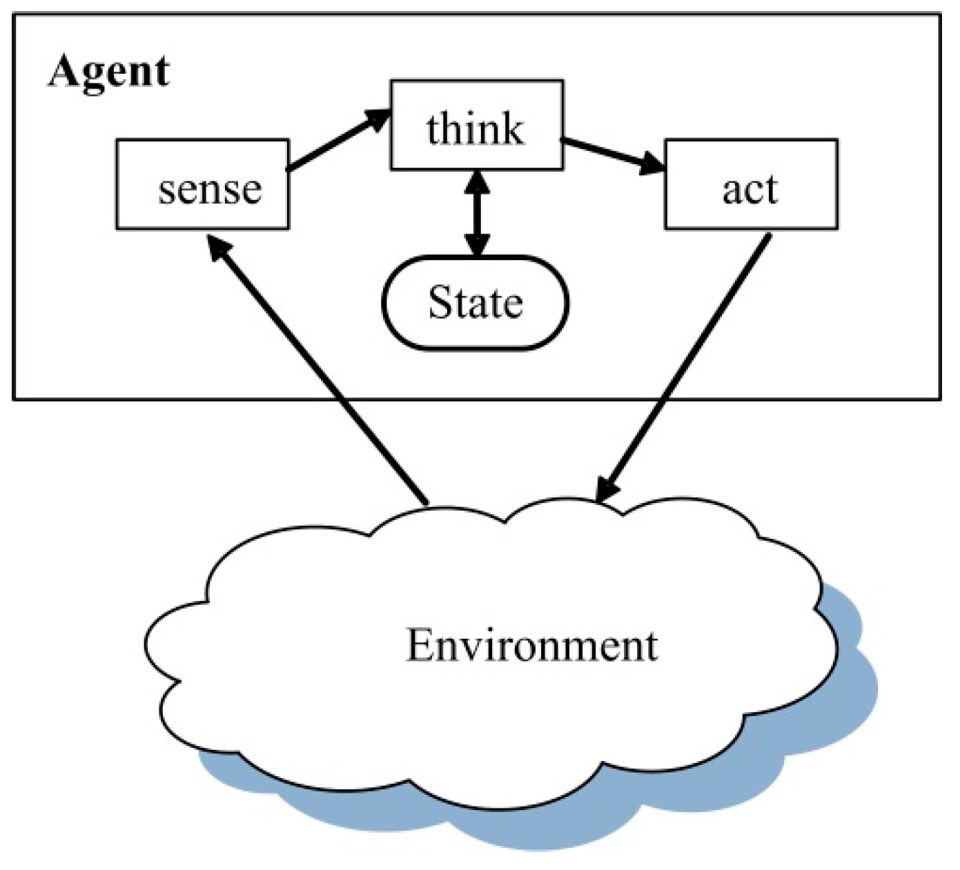
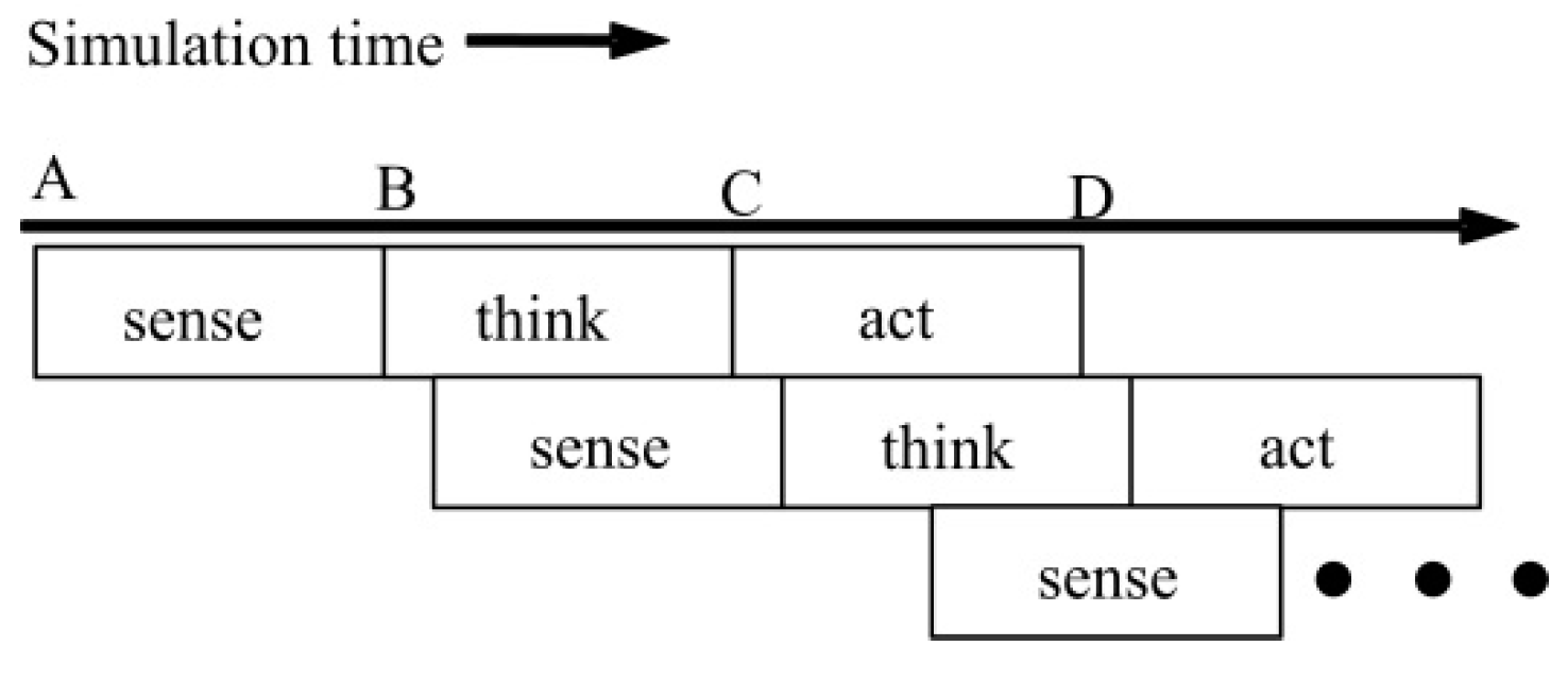
2.1. Traditional Agent Behavior Model

From the structure, an agent consists of the sensor, the actuator, and decision components. The agent uses the sensor to perceive the environment and performs the act determined by the decision components through the actuator, which then affects the environment or other agents. Thus, the agent usually conducts the behavior modeling with the “sense-think-act” cycle, as shown in Figure 1 [4]. Here, the agent first obtains senses from the environment, then processes these senses and thinks about what to do, and finally acts to affect the environment.
The Scalable Agents Simulation System (SASSY) [4] and Parallel Discrete Event Simulation for Multi-Agent System (PDES-MAS) [30] are the main hybrid simulation platforms using this original Traditional agent Behavior Model (original TBM). The System for Parallel Agent Discrete Event Simulator (SPADES) [31] framework improves this model by establishing a “sense-think-act” delay model (which can be shorted as delayed TBM). In this model, an agent cycle consists of the following three steps: sense, think and act, each with a corresponding delay. These delays can be arbitrary, except for the “think” steps, which are not allowed to overlap in two cycles, and different steps of different cycles that can overlap within the delay time, as shown in Figure 2 [31]. The “think” steps are not allowed to overlap because of the assumption that a typical agent only has one Central Processing Unit (CPU) and cannot think at the same time; this model can perceive the external environment while simulating the thinking of the agent.
These two typical TBMs describe the physical agent model intuitively using the cycle formed by the three steps of sense, think, and act. In the war system, the decision cycle based on perception can also be described using this “sense-think-act” paradigm. Among them, sense corresponds to the sensor processing, think corresponds to the process of Command and Control (C2), and act contains the implementation process of behaviors including maneuver, attack/defense, logistics management, and communication.
However, these traditional “sense-think-act” models have some shortcomings in simulating the behavior of agents in a continuous process. From the perspective of information processing, the original TBM regards the agent and its behavior as information processing conducted by a device with an input and output (e.g., the agent’s perception would be the input and its act would be the output). This type of input/output model is mainly for autonomous agents with intelligent acts. Even with the delayed TBM, the assumption that the “think” steps cannot overlap is mainly applicable to agents of the machine type and presents an inability to describe all agent types in a complex system.
For example, some semi-autonomous entities in military simulation can not only determine and carry out an act required to accomplish a goal by sensing the external environment, but also perform actions by strictly following the order of the superior while under the superior’s command and control. In this case, the agent can perform the act without needing to undergo the steps of sensing and thinking.

2.2. State Update Mechanism in Agent-Based Modeling

The state update mechanism is the first problem to be solved before introducing DES in the agent-based model. In each of the “sense-think-act” cycles in the agent model, the agent needs to update its state and complete the synchronization with other agents. Minimizing the number of state updates becomes the key to the efficiency improvement of the hybrid simulation.
According to the ways different simulation models change their states, simulation can be divided into synchronous simulation and asynchronous simulation. In synchronous simulation, all state variables of all entities are updated synchronously. Asynchronous simulation allows an entity to individually update its own state at one specific simulation moment regardless of other entities, while in asynchronous simulation, the asynchronous update for attributes can also be applied; that is, at the state update point, the entity only needs to update variables that have state changes, rather than update all of the state variables.
With the simulation time mechanism and the state synchronization mechanism combined, the updating of the agent’s attributes in the hybrid simulation can be carried out using the following methods [20,32,33]:
(1) Fixed time synchronization (FS): All agents update their respective states at fixed intervals. The smaller the time step, the fewer the interactions missed by the simulation and the more accurate the simulation results. This method is easy to be realized, which is an advantage of fixed time synchronization. However, a drawback is that there may be redundant updates. The small steps used to guarantee the correctness of the simulation results often tremendously increase the number of updates of the agent’s state. Even when there is no event, the agent’s state change still needs to be checked. Moreover, the fixed time step requires the shortest possible interval that might occur for all interactions. As interactions occurring in the battlefield are random, and there are many entities, the computational burden increased by this fixed-step method is too much to meet the requirement of computation efficiency proposed in analytic simulations.
(2) Variable time synchronization (VS): All agents update their states simultaneously, and the update requirements can be proposed by any agent in the simulation. The step size for the agent to update its state is not fixed during the simulation. This method still faces the problem of redundant updates, and has many unnecessary computation processes.
(3) Optimistic synchronization (OS): Each agent updates its state separately without considering other agents, and only if it finds that there has been a causal error caused by the interaction with other agents will it use the rollback mechanism to roll the agent back to its state before the interaction occurs. This method can give full play to the agent’s parallelism, but when too many causal errors occur, the frequent rollback has a great influence on the system’s overall operating efficiency.
(5) Complete resynchronization (CR): At each resynchronization moment, all agents update their states.
(6) Partial resynchronization (PR): At each resynchronization moment, only the required agents update their states.
In these state update mechanisms, FS, VS, and OS are synchronous simulation, and CR and PR belong to asynchronous simulation. All states of all agents in the synchronization simulation need to be updated synchronously. In asynchronous simulation, the agent can update the state variables according to its own state change and conservatively estimate when the interaction will occur, requesting that relevant agents update the states once the interaction occurs; that is, to carry out resynchronization.
The efficiencies of the five state update mechanisms are compared qualitatively in several aspects, including whether they need to update all states, whether or not states of all agents need to be updated, and how to update states, as shown in Table 1. It is worth noting that the measurement of the execution time is not contained because it is not easy to be compared directly without any other influence, especially when a large number of statistical elements are included in the simulation. Comparatively, the indicators in the table can still be used to evaluate efficiency as they reflect the number of operations the agent takes during the simulation.
This shows that the PR method does not require all agents to update all states simultaneously, and the timing of updating the status is at some specific time compared to other state synchronization mechanisms. When the entities are dispersed in military simulation, the number of interactions among entities will be correspondingly small, and the number of required resynchronizations will be small, as well. Therefore, for the large number of entities deployed in the large defense space in a military simulation, the use of the PR mechanism can reduce a large amount of unnecessary state updates.

2.3. Approaches of Combining DES and Agent-Based Modeling

In general, the combination of DES and agent-based modeling can obtain better efficiency than pure MAS. In the existing hybrid simulation, agent-based modeling and DES play different roles. According to the different ways of discretization of a continuous model in MAS, the model pattern of the hybrid simulation can be classified into four categories: strict discrete, complete time-stepped and discrete, partial time-stepped and discrete, and implicit modeling-based discrete.
(1) Strict discrete (SD). The method converts a continuous model strictly to a discrete model [34]. Since the models in the system are all discrete models, this method mainly adopts an asynchronous simulation mechanism such as CR or PR to update the state. Although strict discreteness can improve efficiency, it cannot fully express the dynamics of a continuous model, which should be involved when there is a need for the study of the continuous model in depth.
(2) Complete time-stepped and discrete (CTD). This approach applies a discrete event simulator to an agent-based model. When the behaviors of agents cannot be predicted, discrete events are created based on the time steps. This is a compromise approach. It is based on the similarity of time-driven simulation and event-driven simulation, where discrete events can be used to realize the time-advancing mechanism of time-stepped simulations. This method is consistent with the timed simulation in the realization of continuous model. The state update mechanism can be a synchronous simulation such as FS, VS, and OS. It should be noted that sometimes it is even less efficient than the time-stepped simulation because of the overhead in the operation of events, such as creating, sorting, and deleting.
(3) Partial time-stepped and discrete (PTD). This method allows hybrid discrete-continuous simulation models to coexist explicitly in the simulation. Some continuous models are used to describe unpredictable agent behavior. For example, in the research on human travel simulation [35], where a human is abstracted as an agent, the time steps are used to schedule the course of reaching destinations for pedestrians, and discrete events are adopted to simulate the queuing system of agents when the pedestrians are waiting for a bus. In a SPADES system, the model to interact with the world model is scheduled by a continuous simulator, which advances the simulation time by a small number of time quanta, and the interaction between agents (e.g., sensations and actions) is scheduled by a discrete events simulator [31]. Due to the existence of an explicit continuous model, the state update mechanism of this method is a hybrid mechanism of a synchronous simulation plus an asynchronous simulation, which can improve the efficiency to a certain extent.
(4) Implicit modeling-based discrete (IMD). The continuous models in this method are realized as internally-implicit models, and discrete events are used for explicit updates and interactions [36]. CR and PR can be applied in this pattern to retain dynamics while taking full advantage of DES in efficiency. However, the implementation of this method depends on the purpose of the study and the characteristics of the system to be studied. It is necessary to predict the minimal updates of the implicit model and to design a specialized interface to implement these minimal required moments.
The comparison of the four approaches is shown in Table 2. It can be seen that the application of DES is usually at a cost of overhead in the model implementation. In order to apply the PR to the agent-based model, it is necessary to choose either the strict discrete method or the implicit modeling-based discrete method to implement a continuous system as a discrete one.
In large-scale military simulations with efficiency requirements, the implicit modeling-based discrete method is better than the others to realize the hybrid simulation. In some specific large-scale military applications, it is usually necessary to preserve the dynamics of the system as much as possible for research purposes, and the details that are of little relevance to the purpose of the study can be simplified or discarded. Therefore, the important system dynamics can be modeled implicitly in the agent model, with PR updating the state of the agent.

3. Problem Description

In order to better describe the problems to be solved in our proposed method, we first present the symbol table in Table 3. After a review of the military context, the issues in PR will be discussed in this section.

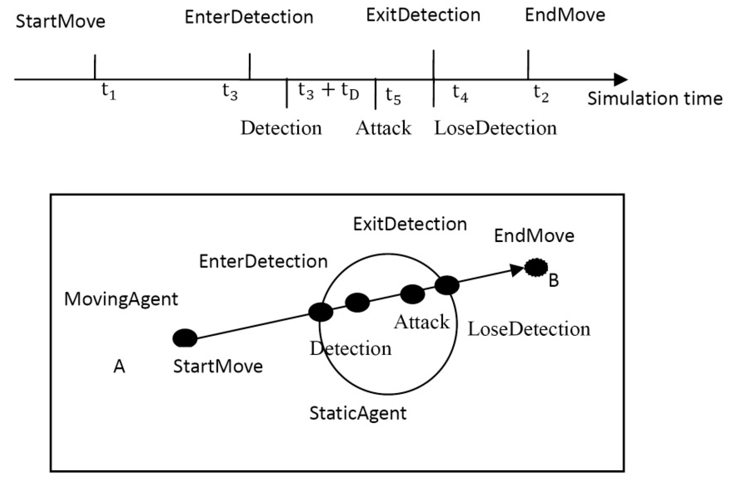
3.1. Context Overview

This section further describes the military context, as well as the need for a hybrid simulation.
In the military context, the typical CAS model can represent military commanders [37,38]. A state-of-the-art military agent model is a perception-based agent model. The commander agent is created to model the ability of command and control, which can be achieved by simulating the commanders’ decision-making process, sensors, weapons, mobile platforms, and communication facilities to conduct processing, detection, lethality, mobility, and communication, respectively [39,40]. For example, in the Joint Warfare System (JWARS) [41], a Battle Space Entity (BSE), which is the basic element to represent military forces and systems, is composed of C2, Sensor, Platform, Resource Manager, and Communication Manager. The sensor uses different detection radii and probabilities to represent different detection capabilities. Weapons have distinct killing probabilities and ranges. The maneuver platforms have their own moving speeds.
In military conflict scenarios, the interactions between agents not only involve the exchange of orders, reports, and requests between the superiors and subordinates in the same side, but also contain a large number of interaction events concerning perception and attack. In general, the commander agent forms the understanding of battlefield situations based on information gathered from its own perception and other commander agents. In light of this cognition, the commander agent completes its decisions and then performs actions such as movement and combat. In turn, the results of these actions are fed back from the environment. On the whole, the process forms a perception-based decision cycle.
Influenced by the numerous entities in the military system and the inundated interaction, the agent-based military simulation has devote much attention to the running efficiency. In particular, when using iterative runs of large samples to provide optimized solutions in the military decision-making system, the quality of the provided options depends on the time available before the submission of the planning [42,43]. The more abundant the time, the more simulations can be carried out, which leads to more experiments carried out in real time. A lot of work has been studied at different levels on how to improve the running efficiency of military simulation. Some use low-resolution models [44]. Some utilize parallel methods or high-performance hardware [45,46]. Some make use of hybrid simulations. The use of DES in large-scale military simulations is common to enhance performance. For example, JWARS and Joint Theater Level Simulation (JTLS) [47] are both discrete event simulations.
Therefore, it is worthy for the researchers to study how to establish a hybrid simulation model in the military context.

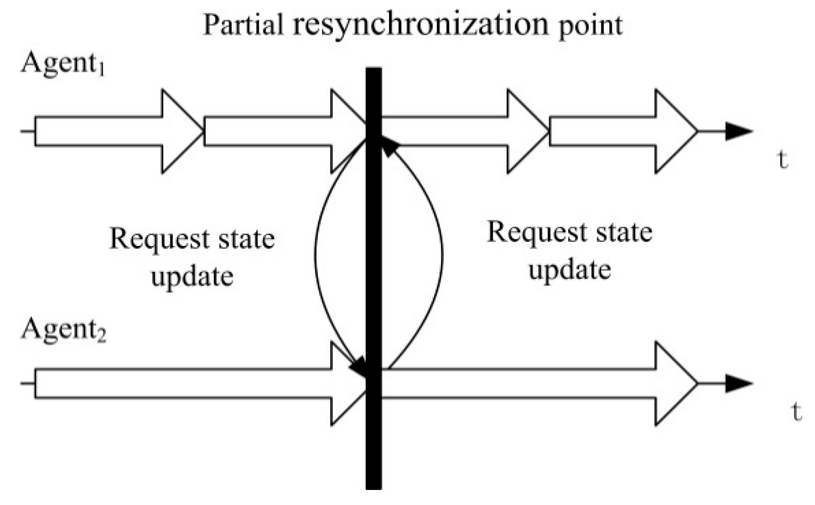
3.2. Main Problems of the PR

From the perspective of the number of updates, partial resynchronization is the method with the minimum number of updates, but there are two important problems that this method possesses, namely, cyclic dependency and the determination of resynchronization intervals.

3.2.1. Resynchronization Interval Determination

The computational efficiency of the resynchronization mechanism is, to a large extent, determined by the setting of the resynchronization interval. Accurately calculated resynchronization events usually mean a larger computation cost on the checking of states [13], while inaccurate resynchronization intervals can lead to incorrect interaction estimation and the loss of interaction information.
There exists a host of solutions to the RI problems. In a study conducted by Kuchar et al. [48] on airspace control, the synchronization interval setting of the uncertain dynamic system was understood as a problem involving signal detection, and the study mainly aimed to minimize false alarms (i.e., premature resynchronization) and lost detection (i.e., the resynchronization process skipped certain interactions). In another approach [20], the measurement agent was designed to predict when an interaction would occur between two related agents as a means of setting the resynchronization interval and determining which agent to be resynchronized, and a “measurement management agent” was used to manage the measurement agent related to many agents. The synchronization time is the minimum value of the next update time predicted by these “measurement management agents”. It was also proposed that the neural network could be used to predict the interaction between two agents.
These methods provide a scheme for determining the estimates of the resynchronization interval, but are not that accurate. If the estimated resynchronization interval is too large, it is possible to miss some actual interactions between agents, which means that some important interactions may be lost. If the estimated resynchronization interval is too small, it is possible to generate more redundant status updates and synchronization.
In the implicit modeling-based discrete approach, the challenge of RI is how to accurately predict the interaction events between the implicit models of two agents. Interactive events can typically be divided into interactions between continuous models, interactions between continuous models and discrete models, and interactions between discrete models. Among them, interaction events directly involved in the discrete models are easier to predict because the moments of the interaction events must be at the discrete time points when the states of the discrete model change.
Therefore, the RI problem has always been an important issue of applying the PR method, whose difficulty lies in predicting the interaction between the implicit modeling of agents.

3.2.2. Cyclic Dependency

Cyclic dependency [49] can be described as direct or indirect dependencies between two or more modules when they perform their own functions.
In partial resynchronization, the environmental state is not described in detail. The state of the agent is updated through the model calculation only when the agent takes the initiative to perform state transition or when it is required by other agents to conduct state updates. The moment a state update is required is referred to as the partial resynchronization point, as shown in Figure 3.
When partial resynchronization occurs between two interdependent agents, this method might involve cyclic dependency. Figure 3 shows the cyclic dependency between two agents. When a g e n t 1 runs to the partial resynchronization point and enters the state update process, as a g e n t 1 and a g e n t 2 interact with each other, the states of a g e n t 1 at this resynchronization point are affected by the states of a g e n t 2 . Thus, a g e n t 1 needs a g e n t 2 to update its ( a g e n t 2 ’s) states. However, the update of the state values of a g e n t 2 is also dependent on the states of a g e n t 1 at the current moment; thus, to carry out a state update, a g e n t 2 requires a g e n t 1 to update its ( a g e n t 1 ’s) states as well. In this dynamic, a cyclic dependency is formed between a g e n t 1 and a g e n t 2 .
Such situations may also occur among N agents: e.g., a g e n t 1 needs a g e n t 2 to update its ( a g e n t 2 ’s) states; a g e n t 2 needs a g e n t 3 to update its ( a g e n t 3 ’s) states, …, a g e n t N 1 needs a g e n t N to update its states, and a g e n t N needs a g e n t 1 to update its states.
Thus, the formal definition of CD can be as follows:
Definition 1. 
(For N agents which are represented as a g e n t 1 ,..., a g e n t i ,..., a g e n t N , there is cyclic dependency between the state of N agents at time t ): t T , if:
s t 1 = δ e x t 1 ( t , s t 2 ) , s t 2 = δ e x t 2 ( t , s t 3 ) , ... , s t i = δ e x t i ( t , s t i + 1 ) , ... , s t N 1 = δ e x t N 1 ( t , s t N ) , s t N = δ e x t N ( t , s t 1 )
where:
  • N 2 and N , is the set of natural numbers,
  • s t i is the states of a g e n t i at time t ,
  • δ e x t i is the external state transition function of a g e n t i .
CD problems can only be triggered by external events. According to Definition 1, the state transition of the agent that occurs in CD is a function of other agent states. This indicates that these state transition functions with external dependencies are external state transition functions of discrete event systems. According to the Discrete Event System Specification proposed by Zeigler [50], discrete event simulation can only change the state of the external state transition function with the occurrence of an external event. This means that the interdependence of state updates between the sender and the receiver at the same simulation event can only be achieved with the arrival of external interaction events.
CD problems are prevalent in PR-based military simulations. A typical example is the calculation of ammunition consumption and force change in military conflict. In the conflict between two or more parties, once a party uses a weapon, the other side will also fight back. During this fight, the combat unit ammunition consumed and the number of soldiers changes until the battle stops. This process is a dynamic and continuous process, with interdependence between combat units involved in the battle. The traditional military simulation uses this process as a continuous state variable, where the states update in a small step-by-step manner based on the initial states of each step. As we have not found any relevant solution after we have tried our best, we think this problem still needs to be addressed for PR.
From the summary in Section 2, it can be seen that the computational efficiency is the key issue for military simulations. Each step in the “sense-think-act” cycle can intuitively describe the physical model in the military domain, but the TBM cannot fully represent entities in the military system, such as semi-autonomous combat units. For a large-scale military simulation, the use of PR mechanism can reduce unnecessary state updates. However, when using the PR mechanism in the practical application process, there are still two important issues that need to be studied: RI and CD.

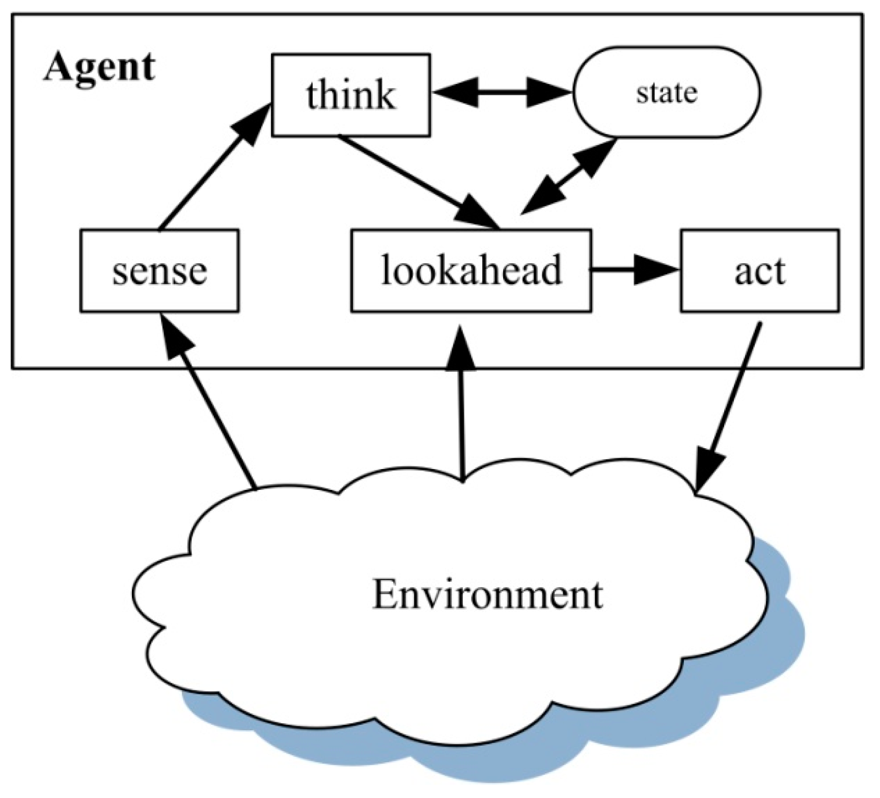
4. The Lookahead Behavior Model

The objective of this paper, in the context of a large-scale military decision-making system application facing running efficiency problems, is to solve the two problems of PR based on the implicit modeling method in order to build a more efficient and feasible hybrid simulation.
The concept of “lookahead behavior” is introduced to the traditional agent behavior model and the “sense-think-lookahead-act” behavior model is proposed, as shown in Figure 4, to solve the two important problems in the process of partial resynchronization and to realize the agent state update model based on an event-driven approach. It can make full use of the advantages of the hybrid simulation composed by the agent model and the DES engine.
A basic aim of LBM is to establish a hybrid simulation based on implicit modeling. The period of the agent behavior model becomes “sense-think-lookahead-act”. Each step of the behavior is based on the corresponding event process as a starting point. The intervals between steps can be arbitrarily delayed, depending on the characteristics of the physical object to be simulated. The initial behavior event of the agent needs to be initialized during the initialization of the simulation. The event for one step is not forced to be created and dispatched during the execution of a previous step in the same cycle. The constraint in the model is that lookahead should be performed right before each action is taken. After the possible interaction during the action is predicted in the lookahead, the action actually performed can be simulated.
The main idea of solving RI in the LBM model is to predict beforehand the likely interaction between agents caused by performing the action. To this end, the authors of this paper propose a time window-based lookahead method.
In order to solve the CD problem in the LBM model, the authors propose a method based on state estimation to break the interdependency cycle of state updates.

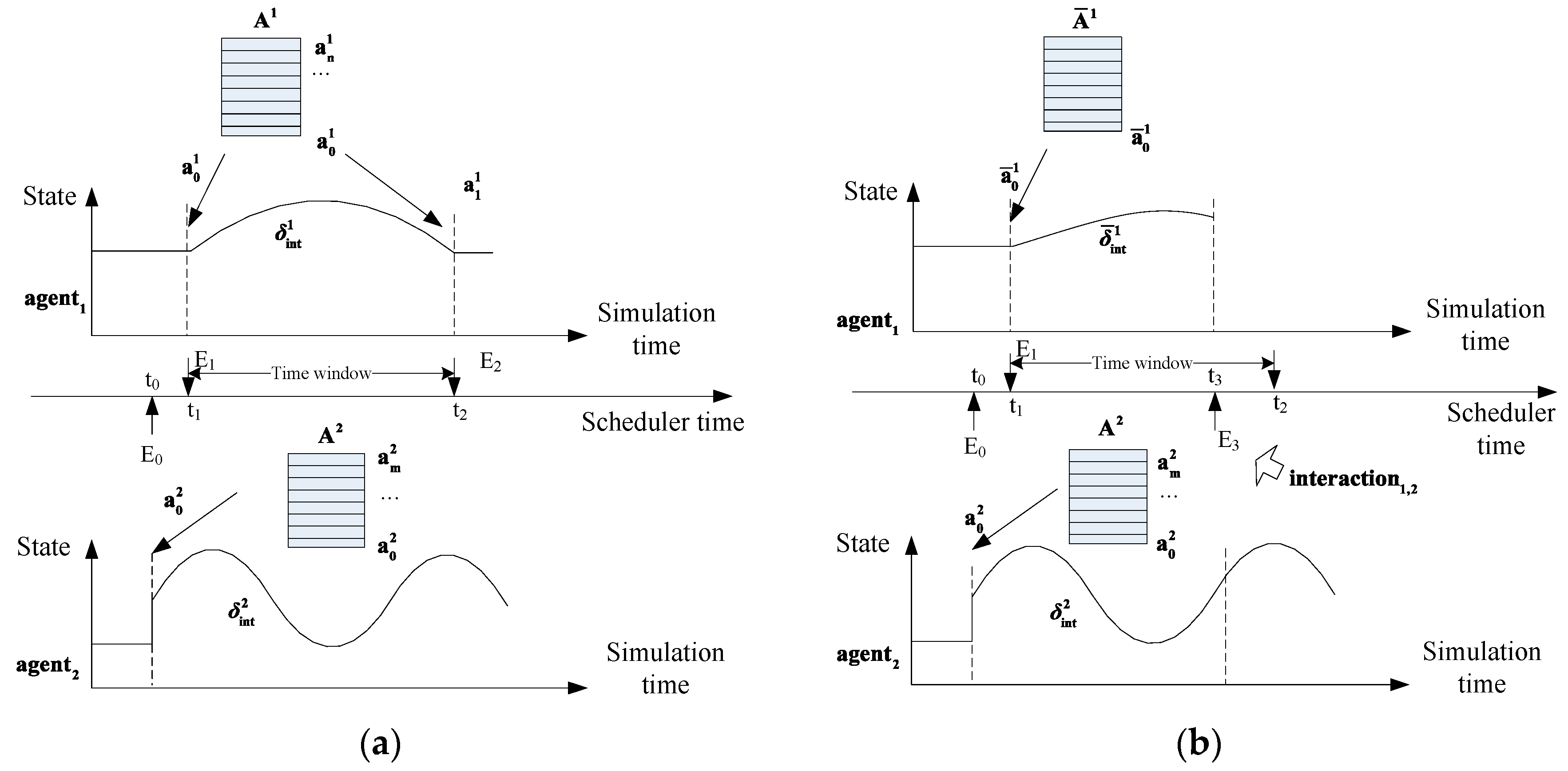
4.1. Time Window-Based Lookahead

The time window-based lookahead is proposed to solve the RI problem. The core of the problem is how to accurately predict the resynchronization interval that may occur between agents in the context of hybrid simulations. In order to fully exploit the efficiency of DES in the background of a military decision-making system, our work is founded on the implicit modeling-based discrete approach. Thus, the issue becomes how to accurately predict the interaction between the implicit models of the two agents.
Further, the interaction events that occur between the implicit models are related to the action being performed by the agent. The change of the internal implicit model corresponds to the change of the internal state transition function of the model. This change is determined only by the action of the model itself. Before the performance of a certain action, the time interval and the corresponding state transition function can be obtained. Therefore, the lookahead process should be finished before each action, in order to predict the interaction between the corresponding internal models of two agents.
The basic idea of the time window-based lookahead is to provide a time window determined by the duration affected by the action and to use the internal model related to the action to determine when the interaction events may happen during that period. The time window and interaction event are defined as follows:
Definition 2. 
(Time window): A time window T w i n d o w in a lookahead step of an agent a g e n t k can be defined as:
T w i n d o w = [ t c u r r e n t , t c u r r e n t + t d u r a t i o n ( a 0 k ) ]
where t c u r r e n t is the current simulation time which satisfies t c u r r e n t = t s t a r t ( a 0 k ) . This means that action a 0 k is the next action to be performed at once for a g e n t k , t d u r a t i o n ( a 0 k ) is the duration of the next action for a g e n t k , and t c u r r e n t + t d u r a t i o n ( a 1 k ) is the end time of the time window, which is also the end time of the next action for the agent.
Definition 3. 
(Interaction event): An interaction event E v e n t k for two agents (referred to as a g e n t k and a g e n t l ) is structured as:
E v e n t k , l = < a g e n t s e n d e r , a g e n t r e c e i v e r , t c r e a t e , t o c c u r , i n t e r a c t i o n k , l >
where:
  • a g e n t s e n d e r is the sender of E v e n t k interaction event, and can be a g e n t k or a g e n t l ;
  • a g e n t r e c e i v e r is the receiver of E v e n t k , and is an alternative choice;
  • t c r e a t e is the creating time of E v e n t k ;
  • t o c c u r is the occurring time of E v e n t k ; and
  • i n t e r a c t i o n k , l represents the corresponding interaction.
In Definition 3, the sender and the receiver of the event can be specified according to the specific kind of interaction, facilitating the sender to trigger the state transition of the receiver.
When a primary updating agent a g e n t k is going to perform its next action a 1 k , there can be two situations for the state change during the performing of a 1 k .
The first one refers to the situation where no other agents interact with the primary updating agent during a 1 k . It is known that action a 1 k initiates a process of internal state transition δ int k , which means the agent will spend time on performing a 1 k . At this point, the state of the primary updating agent can be described as being driven by two events, specifically, the start of the “action” and the end of the “action”. Other state transitions for this action are implied in the internal state transition function δ int k .
For example, in a military simulation of the Anglo-Zulu War [8], Zulu agents can be initialized with a preset movement vector to straight in the direct of the British line. The initial movement vector can be modeled as implicit state transition functions for the states of speed and position. When a Zulu agent starts its movement, it will spend some time on the “moving” action until it arrives at its destination, if not to be replaced by another action of “direct charge”.
The second situation refers to the situation where there are other agents interacting with the primary updating agent. At this point, the state of the primary updating agent is affected by the actions of other agents; therefore, these interactions can be described as events.
As the performance of the action is the “blasting fuse” leading to the change of the agent’s state, the interaction between agents is based on their state. In addition, the determination of the interaction result depends on the act type. Therefore, the interaction between two agents depends on their act and state.
For instance, as the Zulu agent approaches, the British agent sees the enemy troop drawing closer. At this time, the occurrence of the perceiving interaction for the British agent’s perceptual behavior is related to the relative distance between the Zulu agent and the British agent. Only when the Zulu agent is within the detection scope of the British agent will there be a perception interaction between them. Thus, the actions and states of these agents are needed to predict the interactive behavior between agents that may occur using the lookahead process.
The main idea of the time window-based lookahead is based on the “safe” time advancement carried out by the time window, as shown in detail below.
According to Definition 2, a time window is created regarding the sequence of actions to be performed by the agent (which is called the primary agent). Agents associated with it (i.e., agents that may interact with the primary agent) can either “safely” advance to the end of this time window, or can “safely” advance until they interact with each other in this time window. This means that the related agents either will not interact with the primary agent within this time period, or they will conduct time synchronization by generating interaction events within the time window. If an interaction event is generated, then this interaction event may be the input event that changes the primary agent’s state, and the action corresponding to the time window may be affected by this interaction event; thus, the original action of the primary agent will be rescheduled at the moment the interaction event occurs. If there is no interaction event between the primary agent and the related ones in the time window, the primary agent can obtain the state when the action ends, performing its state transition function, and can start performing the next action in the action sequence. By constantly calculating interactions that may occur in the time window, the agent’s action is divided into several sections by the interaction events, and the performance of the agent’s action is going to “jump” in the timeline from one moment to another.
Figure 5 shows a case to explain the basic principle of predicting resynchronization time using the lookahead method. In this example, there are two moving units, which are modeled as a g e n t 1 and a g e n t 2 . The current time of the scheduler is t c u r r e n t . The action sequence of movement to be performed by a g e n t 1 is A 1 = { a 0 1 , .... , a n 1 } , and a g e n t 2 is performing its movement of a 0 2 in its action sequence A 2 = { a 0 2 , .... , a m 2 } at the current moment, where n and m are the numbers of actions to be performed sequentially for a g e n t 1 and a g e n t 2 . The moving speed update functions for a g e n t 1 and a g e n t 2 are modeled as internal state transitions of δ int 1 and δ int 2 , respectively. That is, for a g e n t 1 , the action a 0 1 corresponds to the internal state transition δ int 1 , which will cause a g e n t 1 to change its state from t s t a r t ( a 0 1 ) to t s t a r t ( a 0 1 ) + t d u r a t i o n ( a 0 1 ) . For a g e n t 2 , the state is changed by the internal state transition δ int 2 .
With the change in the speed vector, the spatial positions of agents might change, which could lead to the occurrence of interactions, such as detections.
Without any consideration of interactions between a g e n t 1 and a g e n t 2 , two events for performing action a 0 1 can be created to perform the internal state transition. The “start action” event for a 0 1 is represented as E 0 , while the “ending action” event for a 0 1 is denoted as E 1 . Let t 1 = t s t a r t ( a 0 1 ) , and t 2 = t s t a r t ( a 0 1 ) + t d u r a t i o n ( a 0 1 ) . The initial situation is illustrated in Figure 5a.
After the two events for a 0 1 are scheduled, the time window can be obtained as T w i n d o w = [ t 1 , t 2 ] according to Definition 2. Then, the intersection of functions δ int 1 and δ int 2 can be calculated to generate the i n t e r a c t i o n 1 , 2 between a g e n t 1 and a g e n t 2 within the time window. Supposing that i n t e r a c t i o n 1 , 2 will occur at t 3 , the interaction event will be E 3 = E 1 , 2 = < a g e n t 1 , a g e n t 2 , t 1 , t 3 , i n t e r a c t i o n 1 , 2 > , according to Definition 3. The situation after the lookahead process is illustrated in Figure 5b. It is a remarkable fact that the t 3 is a time in the future, indicating that the event E 3 is a result of the prediction of the lookahead.
In the processing of E 3 , the original state transition for a g e n t 1 might be interrupted. The state of a g e n t 1 will be updated and resynchronized with a g e n t 2 . Meanwhile, the event E 2 could be canceled if the action a 0 1 can only be partially carried out as a ¯ 0 1 . Under the circumstances, the following action sequence of a g e n t 1 will be regenerated at t 3 as A ¯ 1 = ( a ¯ 0 1 ) .
The time window-based lookahead algorithm shown above can be described as Algorithm 1. The duration of action t d u r a t i o n , along with the start time of action t s t a r t , is determined when the action is created. The predictInteraction ( a 0 , a i ) procedure refers to the calculation of the intersection of two internal state transition functions, which are related to a 0 and a i , respectively.
Algorithm 1: Time window-based lookahead algorithm.
Input: next action to be performed at the moment by the primary Agent0: a 0 ; duration of action: t d u r a t i o n
Variables:
                 t c u r r e n t // current simulation time
Output: E v e n t S e t = { ( E v e n t j , S t a t e L o o k a h e a d j ) }
T w i n d o w = [ t c u r r e n t , t c u r r e n t + t d u r a t i o n ]
A g e n t L i s t = getAgentsMayInteractWithAction ( a 0 )
3  for each a g e n t i in the A g e n t L i s t
4      a i = getCurrentPerformingAction( a g e n t i )
5      I n t e r a c t i o n S e t = predictInteraction( a 0 , a i )
6     for each i n t e r a c t i o n j in the I n t e r a c t i o n S e t
7         t j = getPredictedTimeOfInteraction ( i n t e r a c t i o n j )
8         S t a t e L o o k a h e a d j = getPredictedStateOfInteraction( i n t e r a c t i o n j )
9        if( t j T w i n d o w )
10               E v e n t j = createEventFrominteraction( a g e n t 0 , a g e n t i , t j , i n t e r a c t i o n j )
11             E v e n t S e t ( E v e n t j , S t a t e L o o k a h e a d j )
12          end if
13     end for
14  end for
According to Algorithm 1, after the interaction between the primary agent and the other agent in the time window is predicted, the corresponding interaction event can be created according to the predicted time and the agents who participate in the interaction. This lookahead process identifies possible resynchronization interactions within the time window. However, the calculation of the intersection of the internal state transition function may be time-consuming and needs to be optimized according to the actual model. At the same time, the scheduling of interaction events is implemented in the modeling process, so it is necessary to determine all types of interactions between different types of agents before modeling. This aggravates the coupling between models and increases the difficulty of modeling.

4.2. Estimate Value-Based Unlock

The lookahead process described above has realized the prediction of resynchronization time. This sub-section will detail the manner in which the lookahead process solves the problem of cyclic dependency.
The goal of CD in the LBM is to break the cycle of dependency for state updates. This paper proposes a method based on state estimation. The method uses the estimated value for the dependent state to perform the initial state transition calculation, and then uses the final state transition value to replace the estimated one.
The estimated value of state s t k for a g e n t k in this paper is represented as s t k = δ p r e k ( t ) , where t is the moment when the state will occur in future. The estimated state value can solve the CD between the two agents, as shown in the proof of Lemma 1.
Lemma 1. 
Estimated value can eliminate the cyclic dependency between two agents at time t in partial resynchronization.
Proof. 
Assume there is cyclic dependency between a g e n t 1 and a g e n t 2 at a future time t ; that is, the states of a g e n t 1 and a g e n t 2 satisfy s t 1 = δ e x t 1 ( t , s t 2 ) , s t 2 = δ e x t 2 ( t , s t 1 ) .
Then:
i , j , s . t . t i , t j < t , a i 1 ( t i ) A 1 , a j 2 ( t j ) A 2 t i + 1 t , t j + 1 t
namely, the latest actions performed by a g e n t 1 and a g e n t 2 before time t can always be found, and:
s t 1 , s t 2   satisfies   { s t 1 = δ p r e 1 ( t i ) , s t 2 = δ e x t 2 ( t , s t 1 ) , i f t i t j s t 2 = δ p r e 2 ( t j ) , s t 1 = δ e x t 1 ( t , s t 2 ) , i f t i < t j
The following formula can be obtained: s t 1 = δ e x t 1 ( t , s t 2 ) , s t 2 = δ e x t 2 ( t , s t 1 ) ; that is, the states of a g e n t 1 and a g e n t 2 at time t are only related to the state of the lookahead prediction. ☐
According to Lemma 1, the estimated state values can resolve the CD problem between couples of agents (see the proof of Theorem 1).
Theorem 1. 
The estimated value can eliminate the cyclic dependency between agents in partial resynchronization.
Proof. 
If there is cyclic dependency between n agents at time t , then according to Definition 1, the following can be obtained: s t 1 = δ e x t 1 ( t , s t 2 ) , s t 2 = δ e x t 2 ( t , s t 3 ) , , s t n 1 = δ e x t n 1 ( t , s t n ) , s t n = δ e x t n ( t , s t 1 ) .
According to the transitivity of the function, we can determine that: s t 1 = δ e x t 1 ( t , s t 2 ) , s t 2 = δ e x t 2 δ e x t n ( t , s t 3 , , s t n , s t 1 ) . That is, there is cyclic dependency between a g e n t 1 and a g e n t 2 at time t , which could be defined as s t 1 = δ e x t 1 ( t , s t 2 ) , s t 2 = F e x t 2 ( t , s t 1 ) , where F e x t 2 = δ e x t 2 δ e x t n ( t , s t 3 , , s t n , s t 1 ) represents a compound function of t and s t 1 .
From Lemma 1, the estimated value can eliminate the cyclic dependency between a g e n t 1 and a g e n t 2 at time t ; that is, s t 1 , s t 2 can always be found so that s t 1 = δ e x t 1 ( t , s t 2 ) , s t 2 = F e x t 2 ( t , s t 1 ) . Then:
s t 1 = δ e x t 1 ( t , s t 2 ) , s t 2 = δ e x t 2 ( t , s t 3 ) , , s t n 1 = δ e x t n 1 ( t , s t n ) , s t n = δ e x t n ( t , s t 1 )
Thus, it is clear that cyclic dependency no longer exists among the states of the n agents. Therefore, lookahead can eliminate the cyclic dependency between the n agents in partial resynchronization. ☐
Since the CD problem occurs at the moment the interaction event occurs, the time window used to break the dependency loop is a time window of length 0.
Using the estimated value to unlock the state dependencies when updating the state, the problem of how to estimate the status value needs to be addressed. Plenty of time is obviously needed to accurately estimate the state, and the error between the state estimate and the true value will affect the accuracy of the state update. In the present work, the authors of this paper mainly use the method of pre-calculation to save some typical values in some typical scenarios in a local file. Then, the state estimates are interpolated from the typical values so as to achieve a compromise between calculation accuracy and efficiency.

5. Case and Experiments

In order to evaluate the LBM, this paper designs a simple military test case to study the efficiency of different state update mechanisms. The specific assumptions and initial conditions of the experiment are described in Section 5.1. The process of modeling the typical behavior in the scenario is presented in Section 5.2. Then, Section 5.3 gives the experimental results and a brief analysis.

5.1. Case Scenario and Experiment Setup

A simple military air defense scenario is designed with both red and blue units. The red side mainly contains pairs of radar and artillery deployed in the same position, while the units of the blue side are the aircrafts. The detection model of radar uses a simplified constant-delay model based on the detection radius, that is, after the target enters the detection range for a constant time, the radar performs a detection to obtain the target information. The artillery attacks the target after another constant time of the target detection. The damage on the aircraft is not considered. The aircraft’s motion model is a continuous model, using uniform linear motion to update the position. Radar perception and artillery attacks are both discrete models.
In order to simplify the implementation, two types of agents are established: StaticAgent on the red side and MovingAgent on the blue side. StaticAgent simulates the capabilities of detection and attacking of radar and artillery, respectively, whereas MovingAgent simulates the process in which the aircraft performs movements.
Experiments are carried out to simulate the process of sense, move, and attack of the two kinds of agents. The experiment is as follows: set the initial and ending positions of all MovingAgents and perform the moving action a m o v e to move from the initial position to the destination at a fixed speed. When the destination is reached, the agent resets the initial and ending positions and continues the movement. StaticAgent detects the MovingAgents and performs the attack action a a t t a c k .
Four sets of experiments are conducted to evaluate the efficiency of LBM, namely:
(1)
Fixed time synchronization-based simulation (FS);
(2)
Variable time synchronization-based simulation (VS);
(3)
Complete resynchronization-based simulation (CR);
(4)
Partial resynchronization-based LBM simulation (LBM-PR).
In the LBM model, the agent spends its time mainly on performing state updates, executing the behavior cycle, and forecasting the synchronization interval. Assuming that each agent finishes the three tasks for constant time durations, the number of state updates, the number of executed cycles, and the number of lookaheads will affect the time spent by the agent model. Therefore, this paper uses these measurements as the LBM performance indicators. Taking account of random factors, this experiment will use the average of these measurements as the ultimate performance metric.
The parameters of this experiment are shown in Table 4.

5.2. Modeling of Lookahead

In the above scenario, the manner in which the time window-based lookahead process is realized was demonstrated through the interaction between one MovingAgent and one StaticAgent, as follows:
Two agents are in the scenario: the MovingAgent and the StaticAgent, as shown in Figure 6. Current simulation time is t 1 . The MovingAgent is fetching the first action of a m o v e from its action list, as it is going to arrive at point B linearly at constant speed at t 2 . The StaticAgent is an attacking agent located at point C. The sense model of the StaticAgent is a simplified time-delayed sense model with a detection range of R, and a delayed detection time of t D .
According to the sequence of events that an event scheduler processes to advance the simulation clock, the procedure of the lookahead and act of the a m o v e can be simulated as follows:
Step 1: Perform lookahead for a m o v e , current simulation time is t 1 .
Create and schedule the endMoving event E E n d M o v i n g with processing time of t 2 . Create the time window T 1 = [ t 1 , t 2 ] . Then, predict the interactions between the MovingAgent and the StaticAgent during T 1 , which are i n t e r a c t i o n E n t e r D e t e c t i o n and i n t e r a c t i o n E x i t D e t e c t i o n , with occurring time of t 3 and t 4 . Next, create and schedule interaction events E E n t e r D e t e c t i o n and E E x i t D e t e c t i o n .
Step 2: Process event E E n t e r D e t e c t i o n , current simulation time is t 3 .
In this step, the StaticAgent creates and schedules the detection event E D e t e c t i o n at t 3 + t D .
Step 3: Process event E D e t e c t i o n , current simulation time is t 3 + t D .
The StaticAgent performs “sense” behavior, adds the MovingAgent into the target list, and the states are resynchronized between the MovingAgent and the StaticAgent. It is assumed that the StaticAgent decides on an attacking action a a t t a c k at t 5 . Then, the lookahead event E l o o k a h e a d A t t a c k is created and scheduled at t 5 to predict the attacking action’s effect.
Step 4: Process event E l o o k a h e a d A t t a c k ; current simulation time is t 5 .
In this step, the E A t t a c k is created and scheduled attacking action at t 5 .
Step 5: Process event E A t t a c k ; current simulation time is t 5 .
Step 6: Process event E E x i t D e t e c t i o n ; current simulation time is t 4 .
Create and schedule the lose detection event E L o s e D e t e c t i o n for StaticAgent at t 4 .
Step 7: Process event E L o s e D e t e c t i o n ; current simulation time is t 4 .
The StaticAgent performs “sense” behavior; delete the MovingAgents from the target list.
Step 8: Process event E E n d M o v i n g ; current simulation time is t 2 .
The MovingAgent arrives at the destination. The procedure ends, and the action a m o v e is completely performed.
The lookahead process in Step 1 predicts two interactions caused by detection of the StaticAgent, which results in resynchronization between the MovingAgent and the StaticAgent, and divides the moving action into several sub-motions. In Figure 7, the resynchronization between the MovingAgent and the StaticAgent occurs at simulation time t 3 , t 3 + t D , t 5 , and t 4 . In the time window from t 1 to t 2 , the state updates for the MovingAgent are skipped over without any interactions between the MovingAgent and the StaticAgent, except for those at the resynchronization point.

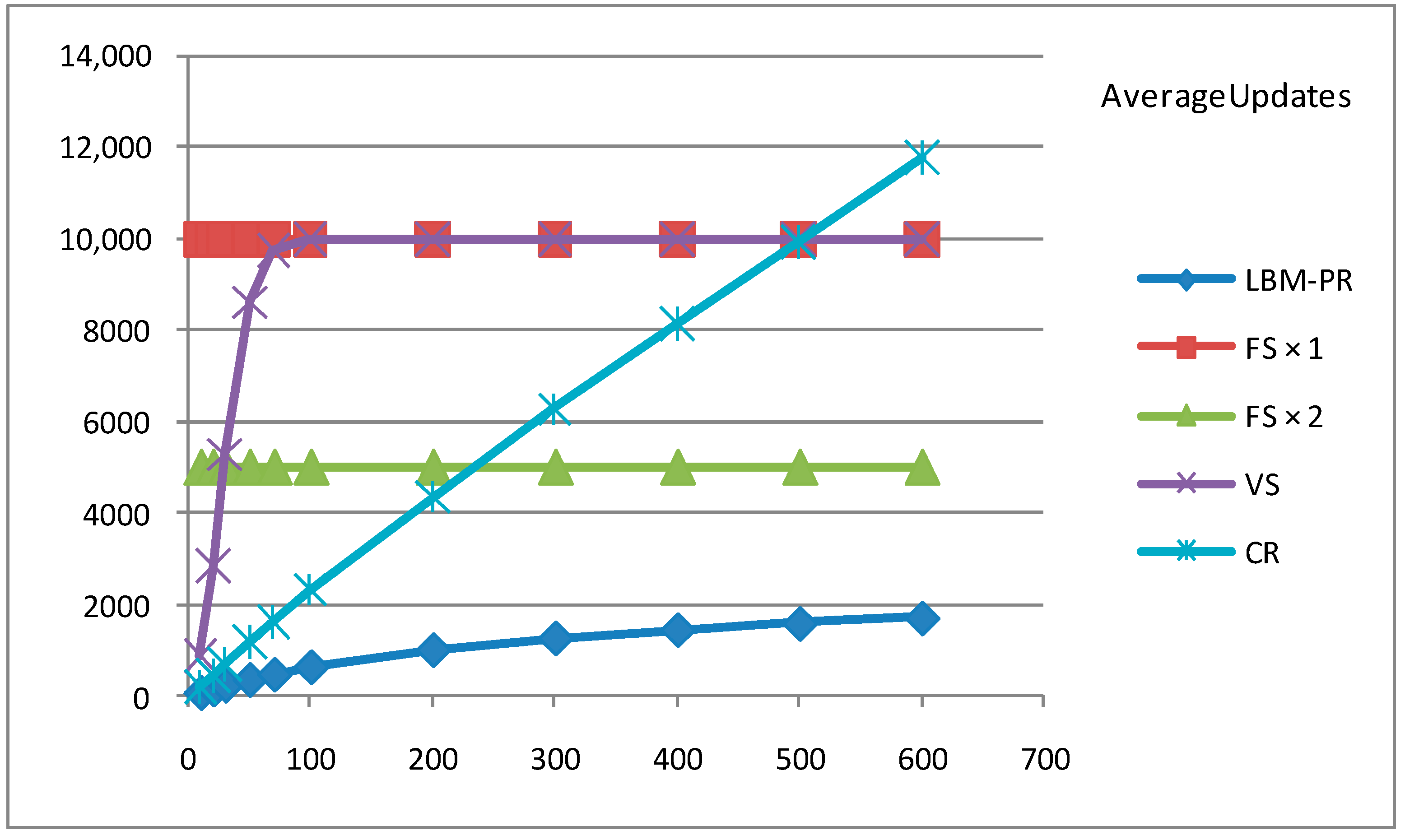
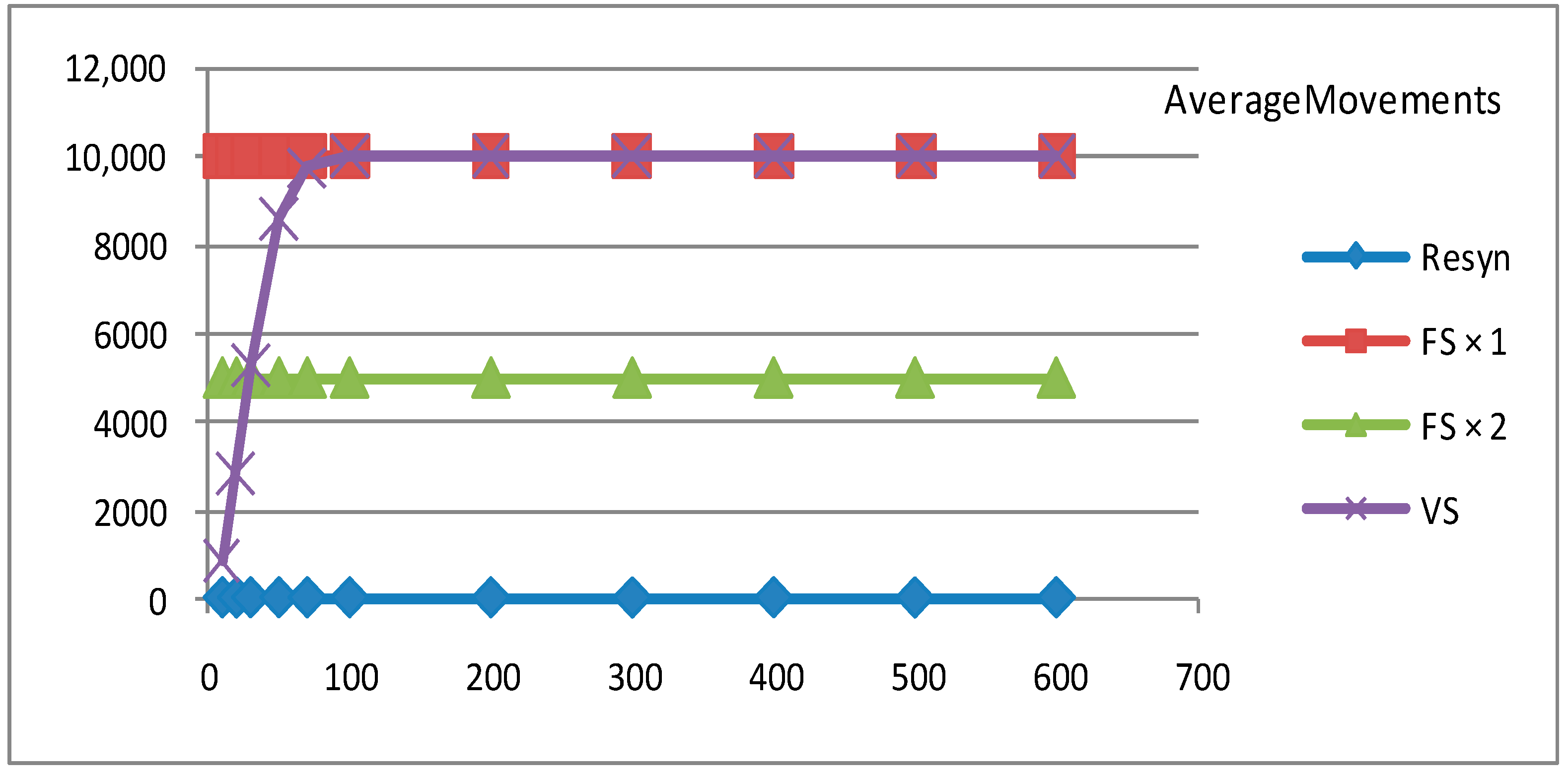
5.3. Experiment Results

The experiments compare the efficiencies of FS, VS, CR, and LBM-PR. We execute the experiments 100 times with the simulation time of 10,000 s, and count the average numbers of updates, movements, and sensations in the four simulations. The minimum time interval for a time-stepped method (e.g., FS, VS) is limited to 1. The experimental results are shown in Figure 8, Figure 9 and Figure 10.
Figure 8, Figure 9 and Figure 10 show the changes of the average number of updates, movements, and sensations with agent numbers when different time mechanisms are used. “FS × 1” in the figures represents the FS simulation with a fixed time step of 1. “FS × 2” represents the FS simulation with a fixed time step of 2. “Resyn” represents the asynchronous simulation including the “CR” and “LBM-PR” methods. Since the average number of movements and the sensation of complete resynchronization and partial resynchronization simulations are the same, the “Resyn” curve is used for both of them in Figure 9 and Figure 10.
The experimental results show that the overall performance of LBM-PR is higher than those of state update mechanisms on the selected samples. Ideally, the number of lookahead occurrences is the same as the number of movements, so that the indicator for movements can reflect that for lookaheads.
It can be seen from the results that:
(1) The counted numbers for the FS are not changed with the increasing number of agents, because every agent updates, senses, and moves at every time step, although there might be more interactions when the total number of agents grows larger.
(2) CR and LBM-PR simulations are superior to the synchronous simulations in efficiency and accuracy for updating the state. Agents in CR and LBM-PR simulations can accurately take their behaviors of “sense” and “move” when, and only when, required. The number of updates is strictly constrained by the time step in the synchronous simulation. The VS method can capture many more interactions than “FS × 2”, as some interactions may happen between the time step of the “FS × 2” method. When some interactions occur between the minimum time intervals, even the VR method will miss them. That is why the average number of updates for CR exceeds the numbers for VR and “FS × 1”.
(3) LBM-PR simulation is superior to CR in the average numbers of updates. At every resynchronization time, all agents update their states in CR, while only some involved agents are required to update in LBM-PR.
(4) The average numbers of movements and sensations for LBM-PR and CR are the same for the same quantities of agents, as the resynchronization only affects the update of the agent but not the motion or sense behavior being performing.
(5) When the number of agents increases from 10 to 100, the average numbers of sensations for VS, CR, and LBM-PR increase obviously. This is because when the size of virtual space stays the same, there are more agents, and thus more interactions between agents. When the number of agents reaches 100, it can be seen from the VR that detection events happen almost at each step on average. At this point, simulations with a fixed step greater than 1 may lose some interactions that occur between two steps.

6. Discussions

This section discusses the characteristics and scope of the LBM proposed in this paper based on a case study.

6.1. Characteristics

The comparisons of LBM with original TBM and delayed TBM are shown in Table 5. Compared to the TBM, the LBM model adds a lookahead step before the action step, and requires that the lookahead must be performed before the action is executed. The implicit modeling of the continuous model makes the links between the steps within a cycle no longer tight, so the delays or overlap relationships between different steps and different cycles become more casual. The continuous models are inside the agent, and the steps of think and sense can be skipped. Therefore, the proposed LBM could be used to model semi-autonomous entities in the military field.
LBM uses a PR-based hybrid simulation paradigm, and has advantages in performance compared with those of the original TBM and delayed TBM. LBM-PR does not need to be updated periodically, and can skip many unnecessary state updates in the continuous model. It will not lose interaction events thanks to the accurate prediction of interaction events.

6.2. Applicable Scope

As mentioned above, the sense, think, and act steps in the LBM model can simulate the sensor detection, commander decision-making, and platform mobility plus weapon lethality, respectively. At the same time, the implicit modeling-based discrete method is used in modeling the dynamics of the system to realize the state transition of the continuous model (such as the movement process). In the lookahead step, the LBM predicts possible interaction events within the time window, according to the actions the agents would take and the corresponding implicit models.
Moreover, LBM can simulate semi-autonomous entities in the military field, or skip the sense step to simulate entities whose self-perceiving capabilities can be ignored in the battlefields. This shows that LBM has the ability to model complex military systems, which include continuous and discrete models.
The implementation of LBM-PR makes LBM take full advantage of the efficient scheduling of DES. This advantage is even more pronounced in systems where the scale is large and the agent behaviors do not change frequently.
However, there are also some disadvantages in efficiency. The event scheduler itself has some overhead in the event scheduling and cancellation. If the frequent changes in behavior lead to the cancellation of a large number of events, it will not only bring additional operating costs for the event scheduler, but also increase the number of invalid lookaheads.
The lookahead process in LBM is closely related to the model. In practice, it is often necessary to simplify the model or optimize the lookahead process according to the research content. In the example discussed in this article, the movement of the MovingAgent is sufficiently simplified, otherwise the overhead of the lookahead itself will increase.
Compared to other methods, LBM increases the difficulty in modeling. Specifically, the time window-based lookahead needs to pre-sort all possible types of events, as well as all possible interactions between agents. The estimated value-based unlock requires the pre-recognition of all possible CDs among all agents, and an estimated state value set or a state prediction function is suggested to be prepared in advance of the simulation. In systems that require a large number of run iterations for decision-making, the estimated value needed to resolve the cyclic dependency should be derived from some statistical values in practice.

7. Conclusions and Future Work

In this study, it is demonstrated that a proposed lookahead behavior model based on a time window could effectively solve the problem of resynchronization interval determination and cyclic dependency in a multi-agent hybrid simulation with partial resynchronization. The implementation process of the lookahead algorithm is described, showing that the lookahead process can eliminate cyclic dependency in the state update process of the agents. This type of behavior model is of great significance to the design and implementation of hybrid simulation, and it is helpful in realizing efficient hybrid simulation systems with a smaller number of agent state updates.
Although the LBM presented in this paper has the ability to model complex military systems and demonstrates better computational efficiency in a given case, the work of this paper still needs to be tested in real-world scenarios. First, the interaction prediction process needs to be optimized in conjunction with real applications, for example, by finding some algorithms to filter the calculation of interactions, which obviously will not happen. Secondly, the performance experiments in more application scenarios will be conducted further to clarify whether and when the performance gains from LBM-PR can offset the overheads of lookahead to a large extent.

Acknowledgments

This study was supported by the National Natural Science Foundation of China (61473300) and the Natural Science Foundation of Hunan Province (2017JJ3371).

Author Contributions

Mei Yang proposed the method and wrote the paper; Yong Peng analyzed the problem; Quan-jun Yin designed the experiments and the structure of the paper; Ru-sheng Ju and Xiao Xu designed the case and performed the experiments; and Ke-di Huang analyzed the case.

Conflicts of Interest

The authors declare no conflict of interest.

References

  1. Riley, P.F.; Riley, G.F. Next Generation Modeling III—Agents:Spades—A Distributed Agent Simulation Environment with Software-in-the-Loop Execution. In Proceedings of the 35th Conference on Winter Simulation: Driving Innovation, New Orleans, LA, USA, 7–10 December 2003; pp. 817–825. [Google Scholar]
  2. Uhrmacher, A.M.; Tyschler, P.; Tyschler, D. Modeling and simulation of mobile agents. Future Gener. Comput. Syst. 2000, 17, 107–118. [Google Scholar] [CrossRef]
  3. Theodoropoulos, G.; Logan, B. A framework for the Distributed Simulation of Agent-Based Systems. In Proceedings of the 13th European Simulation Multiconference (ESM’99), Warsaw, Poland, 1–4 June 1999; pp. 58–65. [Google Scholar]
  4. Hybinette, M.; Kraemer, E.; Xiong, Y.; Matthews, G.; Ahmed, J. Sassy: A design for a scalable agent-based simulation system using a distributed discrete event infrastructure. In Proceedings of the 2006 Winter Simulation Conference—(WSC 2006), Monterey, CA, USA, 3–6 December 2006; pp. 926–933. [Google Scholar]
  5. Sanchez, S.M.; Lucas, T.W. Exploring the world of agent-based simulations: Simple models, complex analyses. In Proceedings of the 2002 Winter Simulation Conference—(WSC 2002), San Diego, CA, USA, 8–11 December 2002; pp. 116–126. [Google Scholar]
  6. Kearns, M.; Singh, S.; Shelton, C.R.; Kormann, D.; Kormann, D. Cobot in lambdamoo: An adaptive social statistics agent. Auton. Agents Multi-Agent Syst. 2006, 13, 327–354. [Google Scholar]
  7. Scogings, C.; Hawick, K.A. Altruism amongst spatial predator-prey animats. In 11th International Conference on the Simulation and Synthesis of Living Systems (ALife XI); Bullock, S., Nobel, J., Watson, R., Bedau, M., Eds.; MIT Press: Winchester, UK, 2008; pp. 537–544. [Google Scholar]
  8. Cioffirevilla, C. Invariance and universality in social agent-based simulations. Proc. Natl. Acad. Sci. USA 2002, 99, 7314–7316. [Google Scholar] [CrossRef] [PubMed]
  9. Scogings, C.; Hawick, K.A. An agent-based model of the Battle of Isandlwana. In Proceedings of the 2012 Winter Simulation Conference—(WSC 2012), Raleigh, NC, USA, 9–12 December 2012; pp. 1–12. [Google Scholar]
  10. Ilachinski, A. Artificial War: Multiagent-Based Simulation of Combat; World Scientific: River Edge, NJ, USA, 2004. [Google Scholar]
  11. Beeker, E.R., III; Page, E.H. A case study of the development and use of a MANA-based federation for studying US border operations. In Proceedings of the 2006 Winter Simulation Conference, Monterey, CA, USA, 3–6 December 2006; pp. 841–847. [Google Scholar]
  12. Wu, S.; Shuman, L.; Bidanda, B.; Kelley, M.; Sochats, K.; Balaban, C. Agent-based discrete event simulation modeling for disaster responses. In Proceedings of the IIE Annual Conference and Expo 2008, Vancouver, BC, Canada, 17–22 May 2008; pp. 1908–1913. [Google Scholar]
  13. Zhang, B.; Chan, W.K.; Ukkusuri, S.V. Agent-based discrete-event hybrid space modeling approach for transportation evacuation simulation. In Proceedings of the Winter Simulation Conference 2011, Raleigh, NC, USA, 11–14 December 2011; Volume 16, pp. 199–209. [Google Scholar]
  14. Bouarfa, S.; Blom, H.A.; Curran, R.; Everdij, M.H. Agent-based modeling and simulation of emergent behavior in air transportation. Complex Adapt. Syst. Model. 2013, 1, 15. [Google Scholar] [CrossRef]
  15. Davis, P.K.; Kahan, J.P. Theory and Methods for Supporting High Level Military Decisionmaking; Rand Corporation: Santa Monica, CA, USA, 2007. [Google Scholar]
  16. Fishwick, P.A.; Kim, G.; Jin, J.L. Improved decision making through simulation based planning. Simul. Trans. Soc. Model. Simul. Int. 1996, 67, 315–327. [Google Scholar] [CrossRef]
  17. Schoemaker, P.J.H. Multiple scenario development—Its conceptual and behavioral foundation. Strat. Manag. J. 1993, 14, 193–213. [Google Scholar] [CrossRef]
  18. Lauren, M.; Stephen, R. Map-Aware Non-Uniform Automata (MANA)—A New Zealand Approach to Scenario Modelling. J. Battlef. Technol. 2002, 5, 27–31. [Google Scholar]
  19. Ross, J.L. A comparative study of simulation software for modeling stability operations. In Proceedings of the 2012 Symposium on Military Modeling and Simulation, Orlando, FL, USA, 26–30 March 2012. [Google Scholar]
  20. Lee, S.; Pritchett, A.R.; Goldsman, D. Hybrid agent-based simulation for analyzing the national airspace system. In Proceedings of the Winter Simulation Conference, Arlington, VA, USA, 9–12 December 2001; pp. 1029–1036. [Google Scholar]
  21. Chan, W.K.V.; Son, Y.J.; Macal, C.M. Agent-based simulation tutorial—Simulation of emergent behavior and differences between agent-based simulation and discrete-event simulation. In Proceedings of the Winter Simulation Conference, Baltimore, MD, USA, 5–8 December 2010; pp. 135–150. [Google Scholar]
  22. Brandolini, M.; Rocca, A.; Bruzzone, A.G.; Briano, C.; Petrova, P. Poly-functional intelligent agents for computer generated forces. In Proceedings of the Winter Simulation Conference, Washington, DC, USA, 5–8 December 2004; pp. 1045–1053. [Google Scholar]
  23. Zhaoxia, W.; Minrui, F.; Dajun, D.; Min, Z. Decentralized Event-Triggered Average Consensus for Multi-Agent Systems in CPSs with Communication Constraints. J. Battlef. Technol. 2015, 2, 248–257. [Google Scholar]
  24. Zeigler, B.P.; Kim, T.G.; Praehofer, H. Theory of Modeling and Simulation, 2nd ed.; Academic Press: San Diego, CA, USA, 2000; p. 474. [Google Scholar]
  25. Zhenhua, W.; Juanjuan, X.; Huanshui, Z. Consensus seeking for discrete-time multi-agent systems with communication delay. IEEE/CAA J. Autom. Sin. 2015, 2, 151–157. [Google Scholar]
  26. Wu, Y.; He, X. Secure Consensus Control for Multi-Agent Systems with Attacks and Communication Delays. IEEE/CAA J. Autom. Sin. 2017, 4, 136–142. [Google Scholar] [CrossRef]
  27. Hou, M.; Zhu, H.; Zhou, M.C.; Arrabito, G.R. Optimizing Operator-Agent Interaction in Intelligent Adaptive Interface Design: A Conceptual Framework. IEEE Trans. Syst. Man Cybern. Part C 2011, 41, 161–178. [Google Scholar] [CrossRef]
  28. Banks, J.; Carson, J.S., II; Nelson, B.L.; Nicol, D.M. Discrete-Event System Simulation, 4th ed.; Person Education: New York, NY, USA, 2005. [Google Scholar]
  29. Qian, X.; Yu, J.; Dai, R. A new discipline of science-the study of open complex giant system and its methodology. Nature 1990, 13, 3–10. [Google Scholar]
  30. Oguara, T.; Chen, D.; Theodoropoulos, G.; Logan, B.; Lees, M. An adaptive load management mechanism for distributed simulation of multi-agent systems. In Proceedings of the IEEE International Symposium on Distributed Simulation and Real-Time Applications, Montreal, QC, Canada, 10–12 October 2005; pp. 179–186. [Google Scholar]
  31. Reifelhoess, P. SPADES: A System for Parallel-Agent, Discrete-Event Simulation; American Association for Artificial Intelligence: Menlo Park, CA, USA, 2003; pp. 41–42. [Google Scholar]
  32. Scogings, C.J.; Hawick, K.A.; James, H.A. Tools and techniques for optimisation of microscopic artificial life simulation models. In Proceedings of the IASTED International Conference on Modelling, Simulation and Optimization, Gaborone, Botswana, 11–13 September 2006; pp. 90–95. [Google Scholar]
  33. Hu, X.; Muzy, A.; Ntaimo, L. A hybrid agent-cellular space modeling approach for fire spread and suppression simulation. In Proceedings of the 37th Conference on Winter Simulation, Orlando, FL, USA, 4–7 December 2005; pp. 248–255. [Google Scholar]
  34. Klingener, J.F. Programming combined discrete-continuous simulation models for performance. In Proceedings of the 28th conference on Winter simulation, Coronado, CA, USA, 8–11 December 1996; pp. 833–839. [Google Scholar]
  35. Dubiel, B.; Tsimhoni, O. Integrating agent based modeling into a discrete event simulation. In Proceedings of the 2005 Winter Simulation Conference—(WSC 2005), Lake Buena Vista, FL, USA, 4–7 December 2005; pp. 1029–1037. [Google Scholar]
  36. Wu, S. Agent-Based Discrete Event Simulation Modeling and Evolutionary Real-Time Decision Making for Large-Scale Systems. Ph.D. Thesis, University of Pittsburgh, Pittsburgh, PA, USA, 2008. [Google Scholar]
  37. Hiniker, P.J. A model of command and control processes for JWARS: Test results from controlled experiments and simulation runs. In Proceedings of the 7th International Command & Control Research & Technology Symposium, Quebec City, QC, Canada, 16–20 September 2002; pp. 1–16. [Google Scholar]
  38. Mason, C.R.; Moffat, J. An agent architecture for implementing command and control in military simulations. In Proceedings of the Winter Simulation Conference, Arlington, VA, USA, 9–12 December 2001; pp. 721–729. [Google Scholar]
  39. Lim, K.L.; Mann, I.; Santos, R.; Tobin, B.; Berryman, M.J.; Abbott, D.; Ryan, A. Adaptive battle agents: Complex adaptive combat models. In Microelectronics, MEMS, and Nanotechnology; SPIE: New York, NY, USA, 2005; pp. 48–60. [Google Scholar]
  40. Hiniker, P. The loaded loop: A complex adaptive systems model of C2 processes in combat. In Proceedings of the RAND Modeling of C2 Decision Processes Workshop, Mclean, VA, USA, 31 July–2 August 2001. [Google Scholar]
  41. Skinner, A.; Mcintyre, G.A. The Joint Warfare System (JWARS): A modeling and analysis tool for the defense department. In Proceedings of the Winter Simulation Conference 2011, Raleigh, NC, USA, 11–14 December 2011; pp. 691–696. [Google Scholar]
  42. Huang, K.D.; Zhao, X.Y.; Yang, S.L.; Yang, M.; Hu, F.H.; Cai, Y. System design description infrastructure overview for military simulation and analysis system. J. Syst. Simul. 2012, 24, 2439–2447. [Google Scholar]
  43. Yang, M.; Zhao, X.-Y.; Cai, Y.; Huang, K.-D. Key technologies of high performance simulation for analytical simulation evaluation. J. Syst. Simul. 2012, 24, 49–53, 81. [Google Scholar]
  44. Liu, B.H.; Huang, K.D. Multi-resolution modeling: Present status and trends. Acta Simul. Syst. Sin. 2004, 16, 1150–1154. [Google Scholar]
  45. Hawick, K.A.; James, H.A.; Scogings, C. High-performance Spatial Simulations and optimisations on 64-bit architectures. In Proceedings of the International Conference on Modeling, Scotland, UK, 24–29 July 2005; pp. 129–135. [Google Scholar]
  46. Bouwens, C.L.; Barnes, S.B.; Pratt, D.; Melim, P. Adapting forces modeling and simulation applications for use on high performance computational systems. In Proceedings of the Spring Simulation Multiconference, Orlando, FL, USA, 11–15 April 2010; p. 148. [Google Scholar]
  47. Prochnow, D.L.; Furness, C.Z.; Roberts, J. The use of the Joint Theater Level Simulation (JTLS) with the High Level Architecture (HLA) to produce distributed training environments. In Proceedings of the Simulation Interoperability Workshop, Orlando, FL, USA, 26–31 March 2000. [Google Scholar]
  48. James, K.K. Methodology for Alerting-System Performance Evaluation. J. Guid. Control Dyn. 1996, 19, 438–444. [Google Scholar]
  49. Jonsson, B.; Perathoner, S.; Thiele, L.; Yi, W. Cyclic dependencies in modular performance analysis. In Proceedings of the ACM International Conference on Embedded Software, Atlanta, GA, USA, 19–24 October 2008; pp. 179–188. [Google Scholar]
  50. Kim, T.G.; Zeigler, B.P. The DEVS Formalism: Hierarchical, Modular Systems Specification in an Object Oriented Framework. Proceedings of 1987 Winter Simulation Conference, Atlanta, GA, USA, 14 December 1987; pp. 559–566. [Google Scholar]
Figure 1. The “sense-think-act” behavior model.
Applsci 07 01095 g001
Figure 2. The agent delay model.
Applsci 07 01095 g002
Figure 3. Cyclic dependency between two agents in partial resynchronization.
Applsci 07 01095 g003
Figure 4. The “sense-think-lookahead-act” behavior model.
Applsci 07 01095 g004
Figure 5. The lookahead principle based on the time window. (a) The initial state. (b) The state after the lookahead procedure.
Applsci 07 01095 g005
Figure 6. The small scenario of the test case.
Applsci 07 01095 g006
Figure 7. The process of the moving action when the MovingAgent is attacked.
Applsci 07 01095 g007
Figure 8. The change of average numbers of updates with agent number.
Applsci 07 01095 g008
Figure 9. The change of average numbers of movements with agent number.
Applsci 07 01095 g009
Figure 10. The change of average numbers of sensations with agent number.
Applsci 07 01095 g010
Table 1. The qualitative comparison of efficiency for the five state update mechanisms (FS: fixed time synchronization, VS: variable time synchronization, OS: optimistic synchronization, CR: complete resynchronization, PR: partial resynchronization).
MechanismAll States Need to Be Updated?All Agents Need to Be Updated?Update Synchronizationly or Not?
FSYesYesSynchronizationly
VSYesYesSynchronizationly
OSYesYesSynchronizationly + Asynchronously rollback
CRNoYesAsynchronously
PRNoNoAsynchronously
Table 2. The comparisons of characteristics for the four approaches of combining DES and agent-based modeling (DES: discrete event simulation; SD: strict discrete, CTD: complete time-stepped and discrete, PTD: partial time-stepped and discrete, IMD: implicit modeling-based discrete).
ApproachesDegree of Utilizing Efficiency Improvement of DESDegree of ImplementationCan Dynamics Be Fully Modeled?Available State Update Mechanism
SDCompletelyHardNotCR/PR
CTDLowSimpleYesFS/VS/OS
PTDRelatively lowRelatively simpleYesFS/VS/OS + CR/PR
IMDCompletelyRelatively hardYesCR/PR
Table 3. Table of symbols.
SymbolNomenclature
N a g e n t s The number of agents in the system
a g e n t k The k th agent, 1 k N a g e n t s
a j k ( t ) The act performed by the k th agent at time t and this action is the j th action it performs, 1 k N a g e n t s
T The time set
t c u r r e n t The current simulation time, t c u r r e n t T
t s t a r t ( a j k ) The start time of the j th action a j k for the k th agent a g e n t k , t s t a r t ( a j k ) T
t d u r a t i o n ( a j k ) The duration of the j th action a j k for the k th agent a g e n t k , t d u r a t i o n ( a j k ) T
s t k The state of the k th agent at time t where 1 k N a g e n t s
s t k ( t c u r r e n t ) The estimated state of the k th agent at time t predicted at time t c u r r e n t where t t c u r r e n t
S k = s t k The set of all the states of the k th agent
s k = s t k The set of all the lookahead states of the k th agent
A j + 1 k = ( a 0 k t 0 , a 1 k ( t 1 ) , , a j k ( t j ) ) The sequence of all actions performed by the k th agent before time t = t j + 1
T ¯ = { t 0 , t 1 , , t j } The set of the beginning time of acts performed by the k th agent before time t = t j + 1
A k = A j k The set of all the actions of the k th agent
A = A k The set of the system’s actions
= S k The set of the system’s states
δ int k : S k S k The internal state transition function of the k th agent
δ e x t k : × T × A S k The external state transition function of the k th agent; it indicates that the state transition of the k th agent occurred at one specific moment is related to the system’s existing acts and states
δ p r e k : × T × A S k The lookahead function of the state of the k th agent; this implies that the state of the k th agent predicted at one specific moment is related to the system’s existing acts and states
F e x t 2 = F e x t 2 ( t , s t 1 ) = δ e x t 2 δ e x t n ( t , s t 3 , , s t n , s t 1 ) A compound function of t and s t 1 for the second agent
Table 4. Experiment configurations.
ParameterValue
Size of virtual space10,000 × 10,000
Number of agents in total10, 20, 30, 50, 70, 100, 200, 300, 400, 500, 600
Speed of MovingAgentRandom number, 1–100
Detection radius of StaticAgentRandom number, 0–50
Table 5. Comparisons of LBM with original TBM and delayed TBM (LBM: lookahead behavior model, TBM: traditional agent behavior model).
AspectsOriginal TBMDelayed TBMLBM
Steps contained in a cycleSense, think, and actSense, think, and actSense, think, lookahead, and act
The relationship of stepsSerial in a cycle, indispensible for each stepSerial in a cycle with arbitrary delays between two steps, indispensible for think stepThink/sense can be skipped, indispensible for lookahead before each action
The relationship of cyclesFixed time intervalArbitrary delayArbitrary
Ability to conduct simultaneouslyNoYes (except for think step)Yes
Number of updatesMoreMoreLess
Number of resynchronizationsMoreMoreLess

