
A Novel Method for Sensorless Speed Detection of Brushed DC Motors


Abstract
:
1. Introduction
- The observers based on the dynamic model estimate the speed using a model of the brushed dc motor. A linear model is usually used [3,4], but this type of model has the problem that the parameters used, such as resistance, inductance, and back electromotive force (back-EMF), change under different operating conditions [5,6]. In this situation, the parameters are adjusted for one specific work condition and they are not modified. Consequently, the observers work correctly when operating conditions are similar to the specified conditions, but they do not work as well when the operating conditions differ from the specified conditions. A first solution for this is to dynamically estimate the parameters of the model [7,8,9], but this generates a complex model that is usually nonlinear. A second solution is to use a nonlinear model of the brushed dc motor [10,11,12], or a technique that indirectly models the motor, such as Neural Networks [13,14] and the Kalman filter [15,16]. The problem with these solutions is that they have a high computational cost, and the estimation of the parameters used is not an easy task. A third solution is to use a method with a simple model that is only valid in a specific condition. For example, the method can model the motor only when the supply turns off [17]. The problem with this method is that the speed can only be measured if the condition is met.
- The observers based on the ripple component use a part of the ac current signal, which is called the ripple component [2,18]. This component is the result of two effects. The first effect is produced because the electromotive force induced in each coil has a sinusoidal shape, and it is not perfectly rectified by the brush-commutator system [19]. The second effect is produced because the brushes in the commutator sometimes short two adjacent commutator segments, joining the terminals of the coils connected to these commutator segments, resulting in peaks in the current [20]. Both effects produce undulations in the current. The number of undulations per second, or ripple frequency, is related to motor speed [21]. Many methods in the literature use the ripple component [2,18,22,23,24,25].
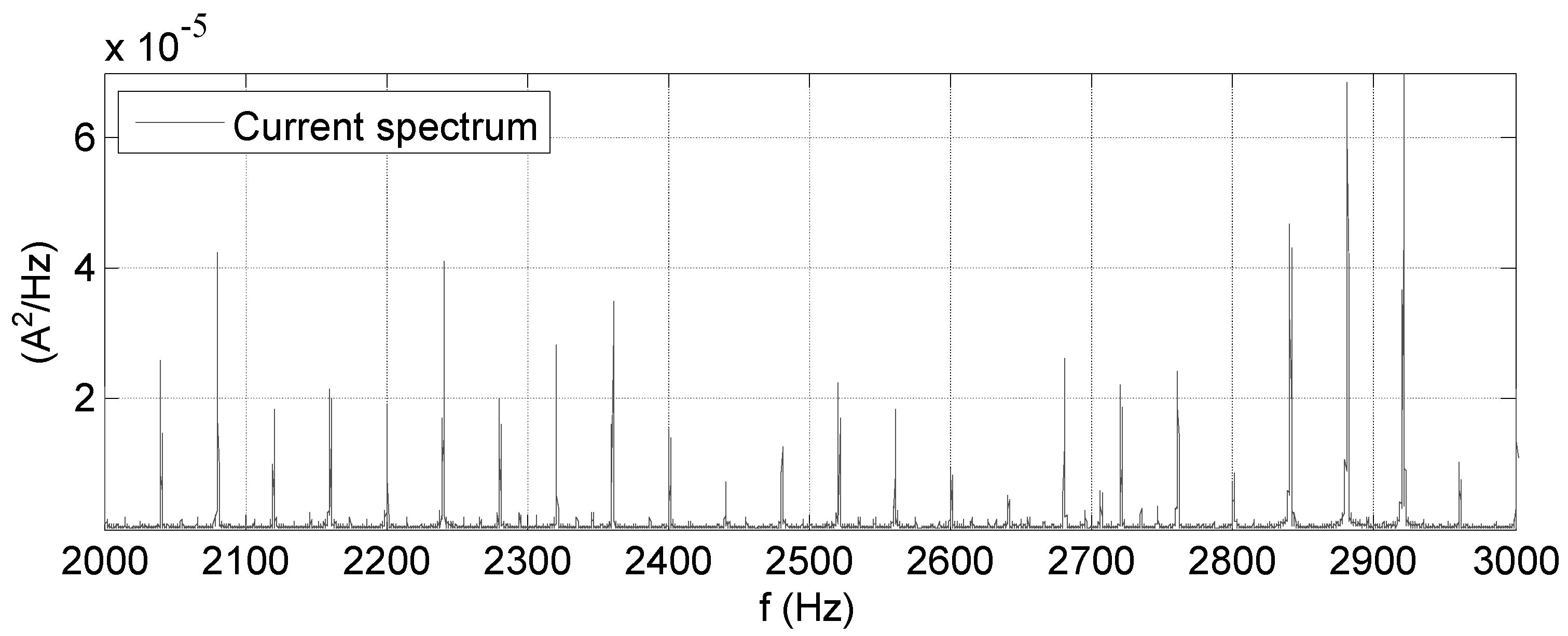
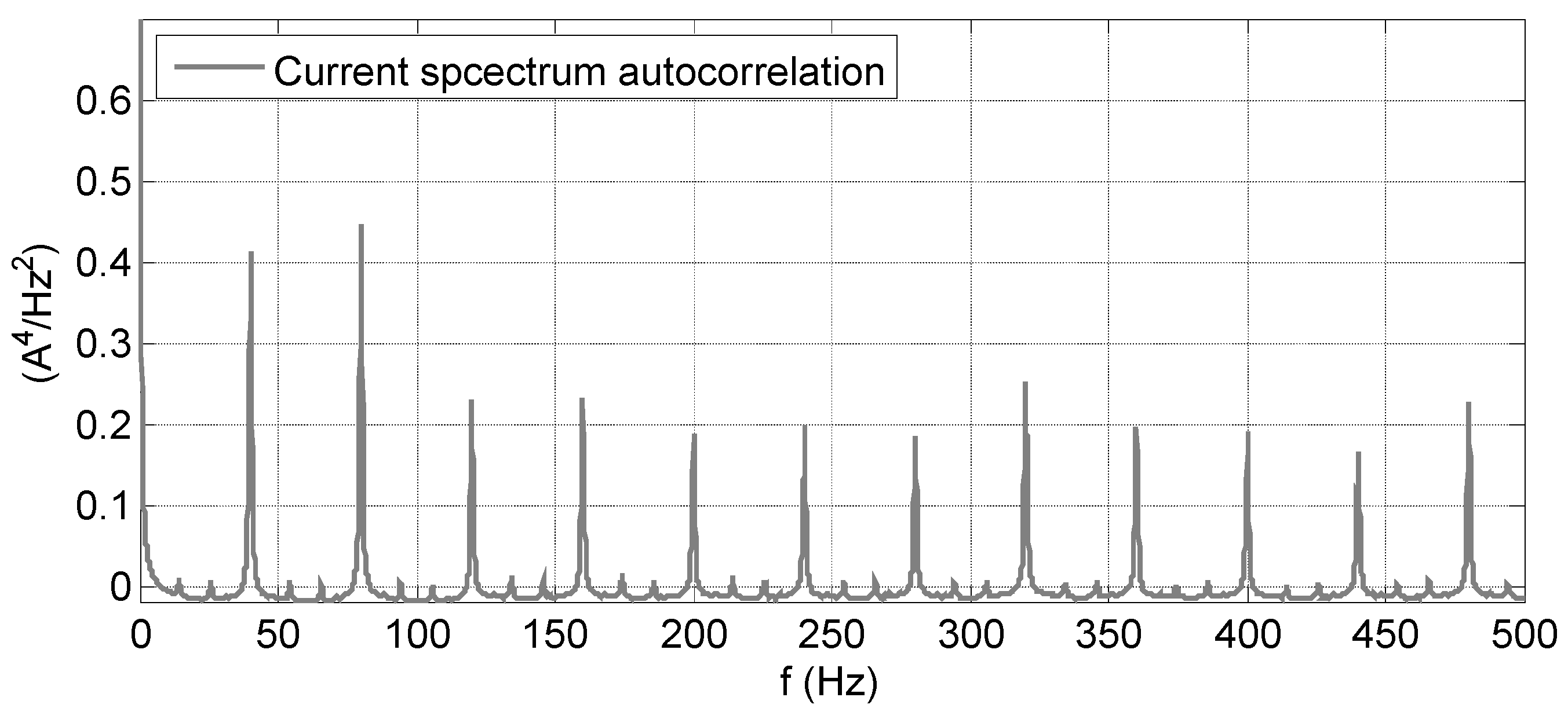
2. Spectral Components of Brushed DC Motor Current
2.1. Ripple Component
2.2. Other Spectral Components
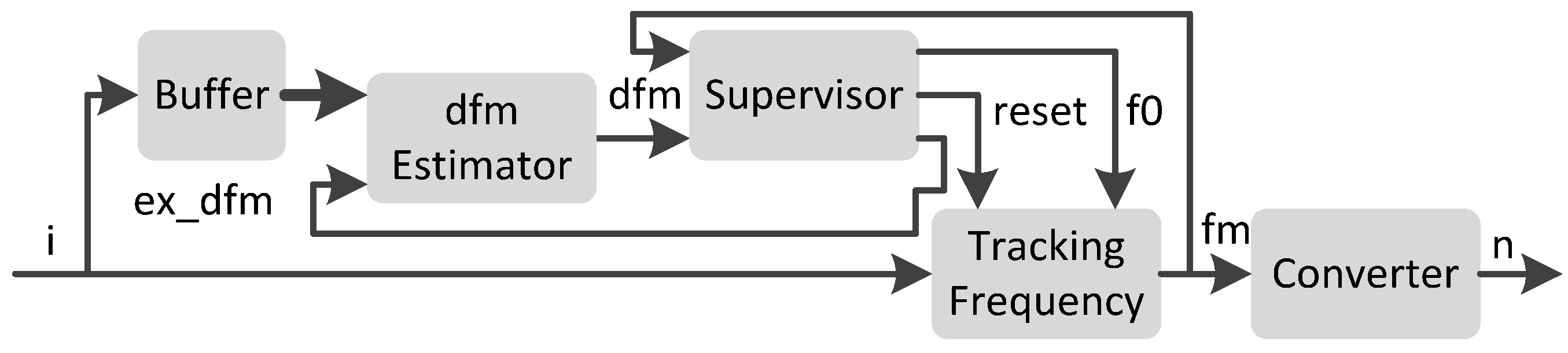
3. Proposed Method
3.1. Buffer Block
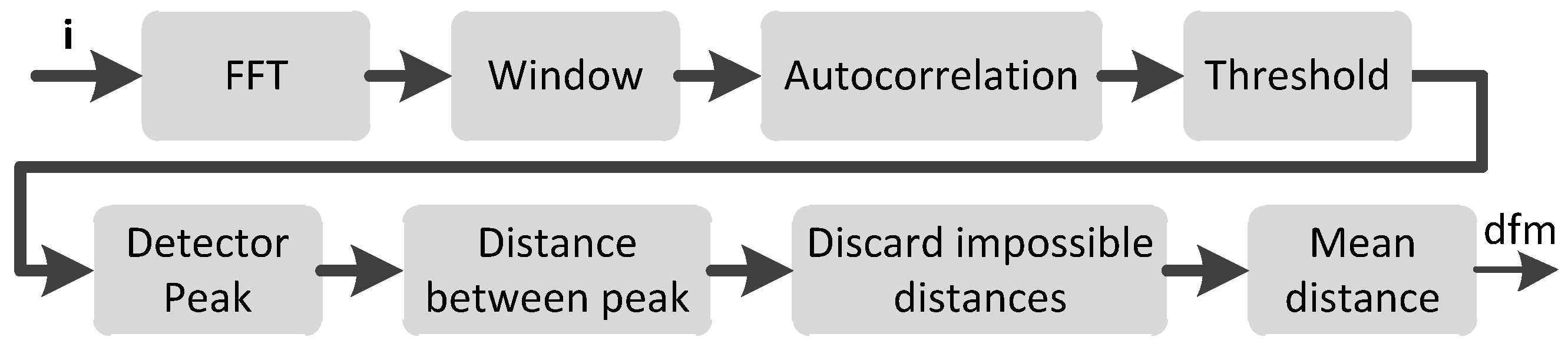
3.2. Estimator Block
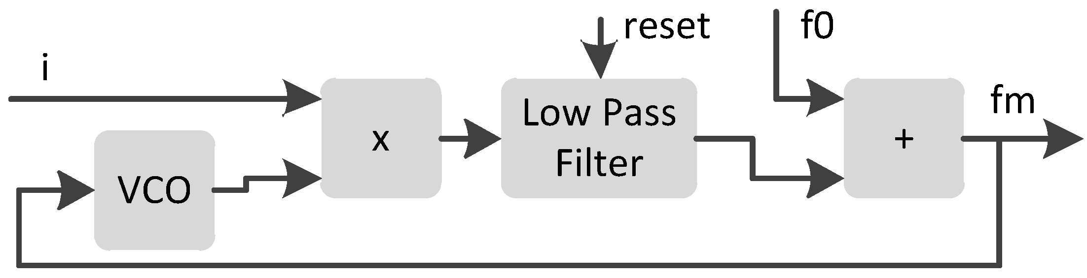
3.3. Tracking Frequency Block
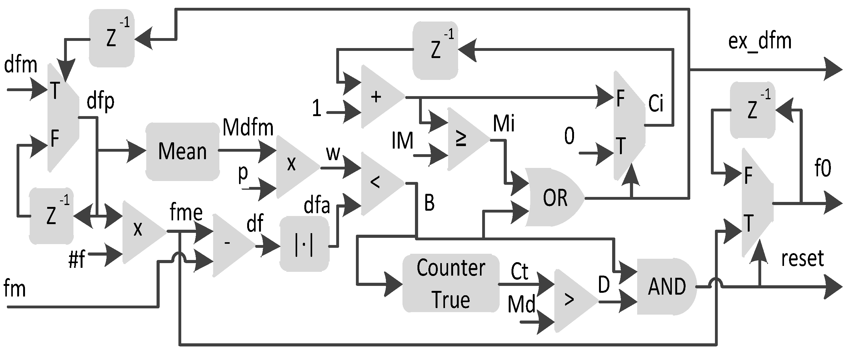
3.4. Supervisor Block
3.5. Converter
4. Experimental Validation
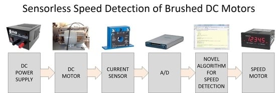
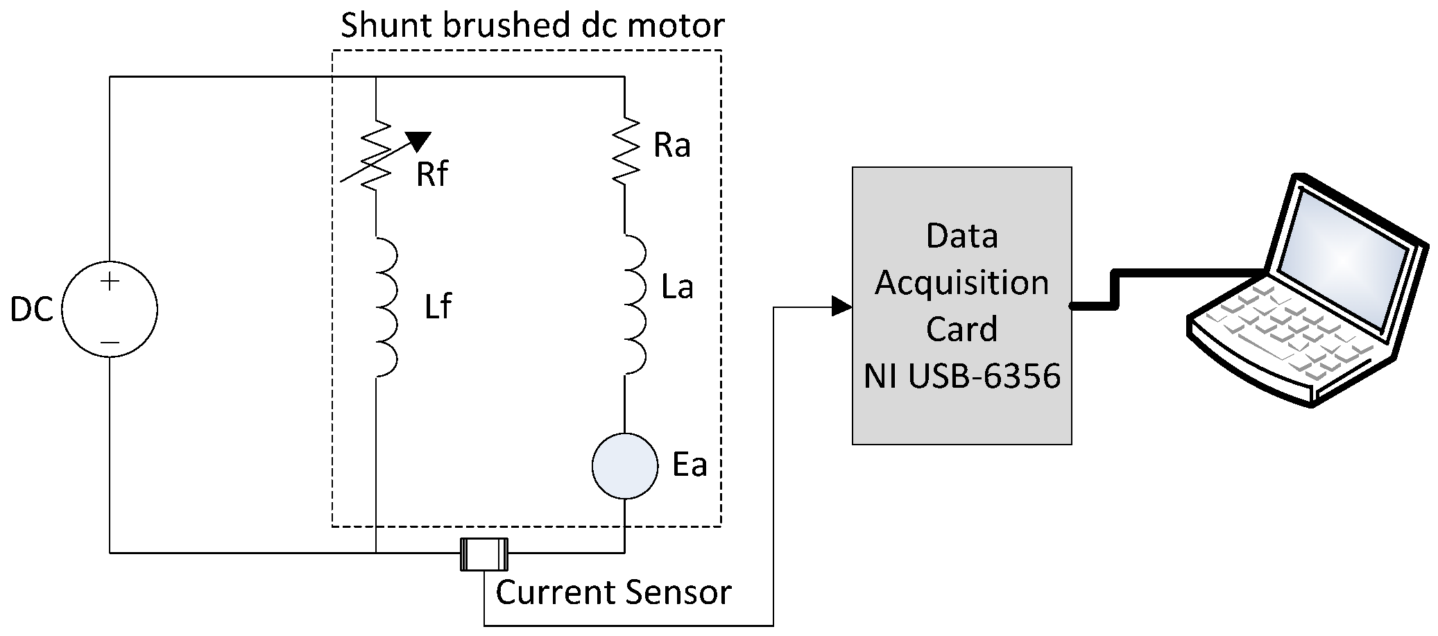
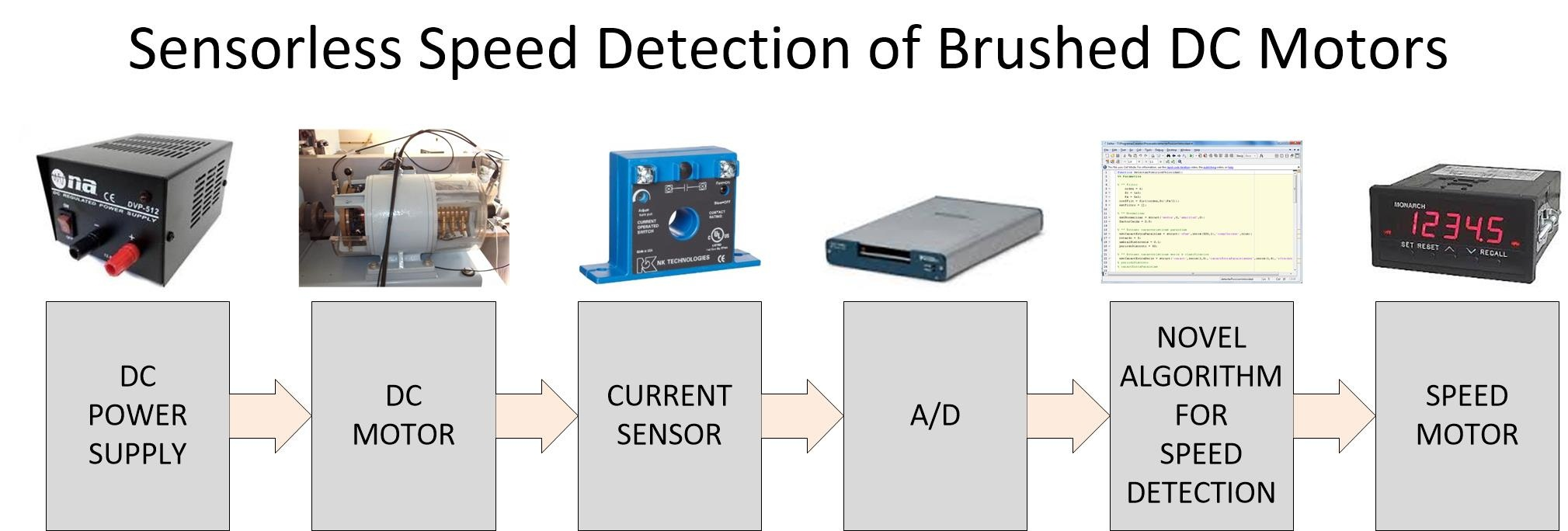
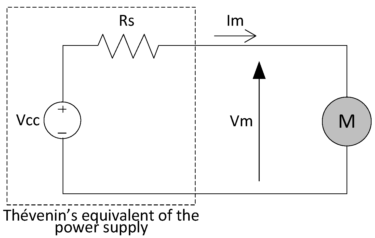
4.1. Description of the System
4.2. Data Collection
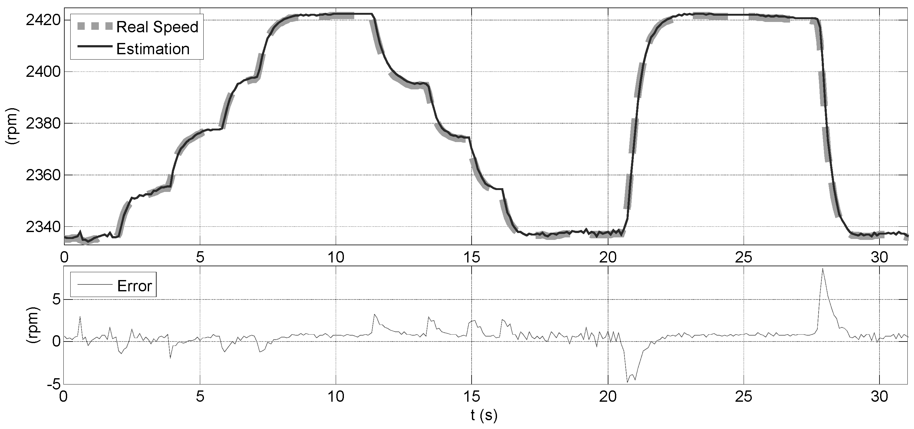
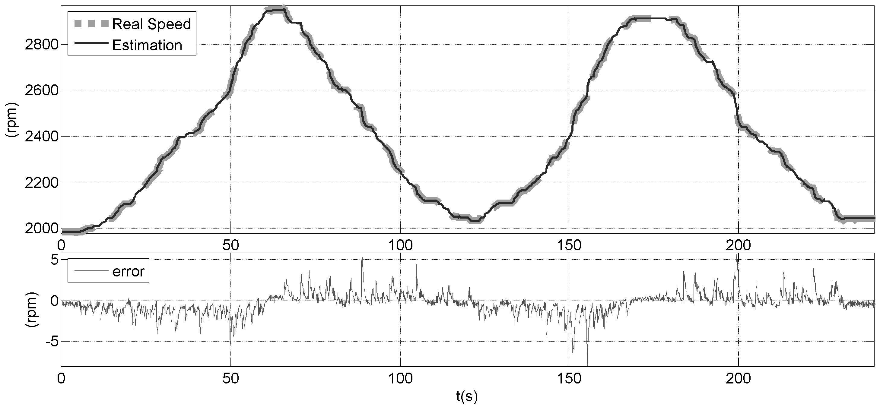
4.3. Comparison of the Predictions with the Measurements
5. Conclusions
- (1)
- It is a novel method that cannot be classified in any of the previous existing sensorless groups; it cannot be classified in either the group of methods based on the dynamic model or the group of methods based on the ripple component. It belongs to a new sensorless group that studies the spectral components of the current and has the advantages of both existing groups.
- (2)
- It requires only the measurement of the current of the brushed dc motor for speed estimation. In contrast, other methods for brushed dc motors with a large number of coils require the measurements of both current and voltage.
- (3)
- It can be used for brushed dc motors with a large number of coils, such as integral horsepower brushed dc motors. In contrast, other methods based on the ripple component that only measure the current can only be used in brushed dc motors with a low number of coils where the ripple component is big enough.
- (4)
- It achieves a low error in speed estimation in the performed tests. Its average error is less than 1 rpm and the standard deviation error is less than 1.5 rpm for speeds between 2000 and 3000 rpm for an H-REM-120-CM motor configured as a brushed dc motor with shunt configuration.
Author Contributions
Conflicts of Interest
References
- Sul, S. Control of Electric Machine Drive System, 1st ed.; Wiley-IEEE Press: Piscataway, NJ, USA, 2011. [Google Scholar]
- Hilairet, M.; Auger, F. Speed sensorless control of a DC-motor via adaptive filters. IET Electr. Power Appl. 2007, 1, 601–610. [Google Scholar] [CrossRef]
- Chevrel, P.; Siala, S. Robust DC-motor speed control without any mechanical sensor. In Proceedings of the IEEE International Conference on Control Applications, Hartford, CT, USA, 5–7 October 1997; pp. 244–246.
- Yachiangkam, S.; Prapanavarat, C.; Yungyuen, U.; Po-ngam, S. Speed-sensorless separately excited DC Motor drive with an adaptive observer. In Proceedings of the IEEE Technical Conference on Computers, Communications, Control and Power Engineering (TENCON 2004), Chiang Mai, Thailand, 21–24 November 2004; Volume D, pp. 163–166.
- Kowal, D.; Patan, M.; Paszke, W.; Romanek, A. Sequential design for model calibration in iterative learning control of DC motor. In Proceedings of the 20th International Conference on Methods and Models in Automation and Robotics (MMAR), Miedzydroje, Poland, 24–27 August 2015; pp. 794–799.
- Lobosco, O.S. Modeling and simulation of DC motors in dynamic conditions allowing for the armature reaction. IEEE Trans. Energy Convers. 1999, 14, 1288–1293. [Google Scholar] [CrossRef]
- Bowes, S.R.; Sevinc, A.; Holliday, D. New natural observer applied to speed-sensorless DC servo and induction motors. IEEE Trans. Ind. Electron. 2004, 51, 1025–1032. [Google Scholar] [CrossRef]
- Cupertino, F.; Pellegrino, G.; Giangrande, P.; Salvatore, L. Sensorless Position Control of Permanent-Magnet Motors With Pulsating Current Injection and Compensation of Motor End Effects. IEEE Trans. Ind. Appl. 2011, 47, 1371–1379. [Google Scholar] [CrossRef]
- Kiyoshi, O.; Yoshihiro, N.; Yoshihisa, H.; Hirokazu, K. High-performance speed control based on an instantaneous speed observer considering the characteristics of a dc chopper in a low speed range. Electr. Eng. Jpn. 2000, 130, 77–87. [Google Scholar]
- Castaneda, C.E.; Loukianov, A.G.; Sanchez, E.N.; Castillo-Toledo, B. Discrete-time neural sliding-mode block control for a DC Motor with controlled flux. IEEE Trans. Ind. Electron. 2012, 59, 1194–1207. [Google Scholar] [CrossRef]
- Liu, Z.Z.; Luo, F.L.; Rashid, M.H. Speed nonlinear control of DC motor drive with field weakening. IEEE Trans. Ind. Appl. 2003, 39, 417–423. [Google Scholar]
- Scott, J.; McLeish, J.; Round, W.H. Speed control with low armature loss for very small sensorless brushed dc motors. IEEE Trans. Ind. Electron. 2009, 56, 1223–1229. [Google Scholar] [CrossRef] [Green Version]
- Farkas, F.; Halász, S.; Kádár, I. Speed Sensorless Neuro-Fuzzy Controller for Brush type DC Machines. In Proceedings of the 5th International Symposium of Hungarian Researchers on Computational Intelligence, Budapest, Hungray, 11–12 November 2004; pp. 147–158.
- Weerasooriya, S.; El-Sharkawi, M.A. Identification and control of a DC motor using back-propagation neural networks. IEEE Trans. Energy Convers. 1991, 6, 663–669. [Google Scholar] [CrossRef]
- Aydogmus, O.; Talu, M.F. Comparison of Extended-Kalman- and Particle-Filter-Based Sensorless Speed Control. IEEE Trans. Instrum. Meas. 2012, 61, 402–410. [Google Scholar] [CrossRef]
- Razi, R.; Monfared, M. Simple control scheme for single-phase uninterruptible power supply inverters with Kalman filter-based estimation of the output voltage. IET Power Electron. 2015, 8, 1817–1824. [Google Scholar] [CrossRef]
- Radcliffe, P.; Kumar, D. Sensorless speed measurement for brushed DC motors. IET Power Electron. 2015, 8, 2223–2228. [Google Scholar] [CrossRef]
- Afjei, E.; Ghomsheh, A.N.; Karami, A. Sensorless speed/position control of brushed DC motor. In Proceedings of the International Aegean Conference on Electrical Machines and Power Electronics (ACEMP’07), Bodrum, Turkey, 10–12 September 2007; pp. 730–732.
- Sincero, G.C.R.; Cros, J.; Viarouge, P. Arc Models for Simulation of Brush Motor Commutations. IEEE Trans. Magn. 2008, 44, 1518–1521. [Google Scholar] [CrossRef]
- Figarella, T.; Jansen, M.H. Brush wear detection by continuous wavelet transform. Mech. Syst. Signal Process. 2007, 21, 1212–1222. [Google Scholar] [CrossRef]
- Yuan, B.; Hu, Z.; Zhou, Z. Expression of sensorless speed estimation in direct current motor with simplex lap winding. In Proceedings of the IEEE International Conference on Mechatronics and Automation, (ICMA 2007), Harbin, China, 5–8 August 2007; pp. 816–821.
- Lott, J.; Burke, D. Brushed Motor Position Control Based Upon Back Current Detection. U.S. Patent 20060261763 A1, 23 November 2006. [Google Scholar]
- Won-Sang, R.; Hye-Jin, L.; Jin Bae, P.; Tae-Sung, Y. Practical Pinch Detection Algorithm for Smart Automotive Power Window Control Systems. IEEE Trans. Ind. Electr. 2008, 55, 1376–1384. [Google Scholar]
- Micke, M.; Sievert, H.; Hachtel, J.; Hertlein, G. Method and Device for Measuring the Rotational Speed of a Pulse-Activated Electric Motor Based on a Frequency of Current Ripples. U.S. Patent 7265538 B2, 4 September 2007. [Google Scholar]
- Vazquez-Sanchez, E.; Gomez-Gil, J.; Rodriguez-Alvarez, M. Analysis of three methods for sensorless speed detection in DC motors. In Proceedings of the IEEE International Conference on Power Engineering, Energy and Electrical Drives (POWERENG ‘09), 18–20 March 2009; pp. 117–122.
- Kessler, E.; Schulter, W. Method for Establishing the Rotational Speed of Mechanically Commutated DC Motors. U.S. Patent 6144179 A, 7 November 2000. [Google Scholar]
- Vazquez-Sanchez, E.; Gomez-Gil, J.; Gamazo-Real, J.C.; Diez-Higuera, J.F. A new method for sensorless estimation of the speed and position in brushed dc motors using support vector machines. IEEE Trans. Ind. Electron. 2012, 59, 1397–1408. [Google Scholar] [CrossRef]
- Moller, D.D.; Schneider, P.K.; Canales, S.A. Voltage-Sensitive Oscillator Frequency for Rotor Position Detection Scheme. U.S. Patent 7352145 B2, 1 April 2008. [Google Scholar]
- Toliyat, H.A.; Kliman, G.B. Handbook of Electric Motors; CRC Press: Boca Raton, FL, USA, 2004. [Google Scholar]
- Chiasson, J. Modeling and High Performance Control of Electric Machines, 1st ed.; Wiley-IEEE Press: Hoboken, NJ, USA, 2005. [Google Scholar]
- Yarlagadda, R.K.R. Analog and Digital Signals and Systems, 1st ed.; Springer Publishing Company, Incorporated: Stillwater, OK, USA, 2009. [Google Scholar]
- Egan, W. Phase-Lock Basics, 2nd ed.; Wiley-IEEE Press: Hoboken, NJ, USA, 2007. [Google Scholar]


| Speed (rpm) | Average Error | Deviation Error | ||
|---|---|---|---|---|
| Absolute (rpm) | Relative (%) | Absolute (rpm) | Relative (%) | |
| 2004 | 0.141 | 0.007 | 0.319 | 0.016 |
| 2103 | 0.146 | 0.007 | 0.425 | 0.020 |
| 2204 | 0.159 | 0.007 | 0.402 | 0.018 |
| 2297 | 0.089 | 0.004 | 0.286 | 0.012 |
| 2400 | 0.008 | 0.001 | 0.188 | 0.008 |
| 2500 | 0.173 | 0.007 | 0.214 | 0.009 |
| 2603 | 0.241 | 0.009 | 0.371 | 0.014 |
| 2705 | 0.183 | 0.007 | 0.380 | 0.014 |
| 2803 | 0.111 | 0.004 | 0.224 | 0.008 |
| 2913 | 0.254 | 0.009 | 0.114 | 0.004 |
| 2998 | 0.336 | 0.011 | 0.112 | 0.004 |
© 2016 by the authors; licensee MDPI, Basel, Switzerland. This article is an open access article distributed under the terms and conditions of the Creative Commons Attribution (CC-BY) license (http://creativecommons.org/licenses/by/4.0/).
Share and Cite
Vazquez-Sanchez, E.; Sottile, J.; Gomez-Gil, J. A Novel Method for Sensorless Speed Detection of Brushed DC Motors. Appl. Sci. 2017, 7, 14. https://doi.org/10.3390/app7010014
Vazquez-Sanchez E, Sottile J, Gomez-Gil J. A Novel Method for Sensorless Speed Detection of Brushed DC Motors. Applied Sciences. 2017; 7(1):14. https://doi.org/10.3390/app7010014
Chicago/Turabian StyleVazquez-Sanchez, Ernesto, Joseph Sottile, and Jaime Gomez-Gil. 2017. "A Novel Method for Sensorless Speed Detection of Brushed DC Motors" Applied Sciences 7, no. 1: 14. https://doi.org/10.3390/app7010014
APA StyleVazquez-Sanchez, E., Sottile, J., & Gomez-Gil, J. (2017). A Novel Method for Sensorless Speed Detection of Brushed DC Motors. Applied Sciences, 7(1), 14. https://doi.org/10.3390/app7010014