1. Introduction
Historical ecology research is increasingly valuable in assessing long-term baselines and understanding long-term ecological changes, and is increasingly applicable to management, decision-making, and conservation. When ecological survey data are lacking, historical data can be exploited to build mathematical models to supply scientifically meaningful information despite limitations in precision.
Soaring demands for food, fresh water, fuel, and timber have contributed to dramatic environmental changes. Nearly two-thirds of Earth’s life-supporting ecosystems—including clean water, pure air, and a stable climate—are being degraded by unsustainable use. Many scientific studies have come to the conclusion that there is growing stress on Earth’s biological systems. More and more warning signs are appearing. Is Planet Earth truly nearing a global tipping point? Is such an extreme state inevitable? Very few global models are proposed to address those claims and questions. As a result, society is more and more interested in developing mathematical models to assess and forecast the environmental and biological health conditions of our planet.
In Reference [
1], the article presents two specific quantitative modeling challenges in their call for better predictive models:
(1) To improve bio-forecasting through global models that embrace the complexity of Earth’s interrelated systems and include the effects of local conditions on the global system and vice versa.
(2) To identify factors that could produce unhealthy global state shifts and to show how to use effective ecosystem management to prevent or limit these impending state changes.
Determining whether global models can be built using local or regional components of the Earth’s health that predict potential state changes is a huge challenge. Then, based on the potential impact on Earth’s health, how can the global models help decision-makers design effective policies?
The “Nature” article [
1] and many others point out that there are several important elements at work in the Earth’s ecosystem (e.g., local factors, global impacts, multi-dimensional factors and relationships, varying time and spatial scales). There are also many other factors that can be included in a predictive model—human population, resource and habitat stress, habitat transformation, energy consumption, climate change, land use patterns, pollution, atmospheric chemistry, ocean chemistry, biodiversity, and political patterns such as social unrest and economic instability. Paleontologists have studied and modeled ecosystem behavior and response during previous cataclysmic state shifts and thus historic-based qualitative and quantitative information can provide background for future predictive models. However, it should be noted that human effects have increased significantly in our current biosphere situation.
Reference [
2] introduced the “WORLD3” model, which is based on system dynamics—a method for studying the world that deals with understanding how complex systems change over time. Internal feedback loops within the structure of the system influence the entire system’s behavior. However, the model does not make the prediction; rather, it is a tool for understanding the broad sweeps and the behavioral tendencies of the system.
Scientists realize that it is very important to assess and predict the potential state changes of the planetary health systems. Nowadays, there is considerable research [
3,
4,
5,
6,
7,
8] being conducted that takes local habitats and regional factors into account. However, since the article [
1] published in “Nature” called for better predictive models in 2012, there have been few models addressing the problem of predicting long-range and global impacts based only on local factors. Using current models, decision-makers cannot be adequately informed about how their provincial polices may impact the overall health of the planet. Many existing models cannot determine the long-range impacts of potential policies without considering the complex global factors, the complex relationships, and the cross effects in biological systems. The system complexities are manifested in multiple interactions, feedback loops, emergent behaviors, and impending state changes or tipping points. As is well known, suggesting suitable potential policies is very important for the sustainable ecological development of our planet. However, the first step should be to determine those critical factors that affect the global state. Based on the idea above, this paper aims at proposing a framework to model and assess the interactive roles of the local factors, to determine the critical factors and to suggest potential management for the ecosystem’s health.
2. Problem Definition and Model Design
2.1. Defining the Problem
With the rapid economic development, the level of energy demand is rapidly increasing, which results in a series of environmental problems. Both urban and rural ecosystems have to carry out environmental performance evaluation in energy utilization to reconcile economic growth with ecological preservation. We focus on the following considerations:
- (1)
How to construct a dynamic global network model that includes dynamic elements to predict future states of ecological health.
- (2)
How to determine the critical factors that reflect the relationship between the model and the predictive measure.
- (3)
How to determine a feedback policy that reflects the influence of human factors.
2.2. Basic Assumptions
There are so many elements that could be included in the ecological modeling. For simplicity, we make the following assumptions:
- (1)
The state changes over the years and we can observe these state changes.
- (2)
The k – th factor at the t moment is influenced by the same factor at the t − 1 moment and interactive factors in neighborhood at the t moment; we ignore the influence between the different factors at the t − 1 moment. There has been Markov property.
- (3)
The relative influence between one factor and another factor just reflects the ratio of two value changes.
- (4)
To simplify the model, we select several typical factors.
- (5)
Outside factors such as “universe perishing”, a destructive earthquake, and a volcanic eruption will not be considered.
- (6)
Each factor has affected other factors and vice versa. The influence is regarded as directive.
- (7)
The CO2 content could reflect environmental changes.
- (8)
The oil consumption could reflect the source consumption.
- (9)
The population would reflect the bearing capacity of the ecosystem.
- (10)
The electricity would reflect the power consumption.
- (11)
The morbidity rate would reflect threats to life.
- (12)
The Gross Domestic Product (GDP) would reflect the level of wellbeing.
2.3. Symbol Lists
In the concrete implementation of the proposed framework, only four typical factors are utilized in the ecological modeling, as denoted in
Table 1 and
Figure 1. As we adopt the Markov model to predict the dynamic elements, there are also four corresponding symbols to represent their respective predictions.
2.4. Model Design
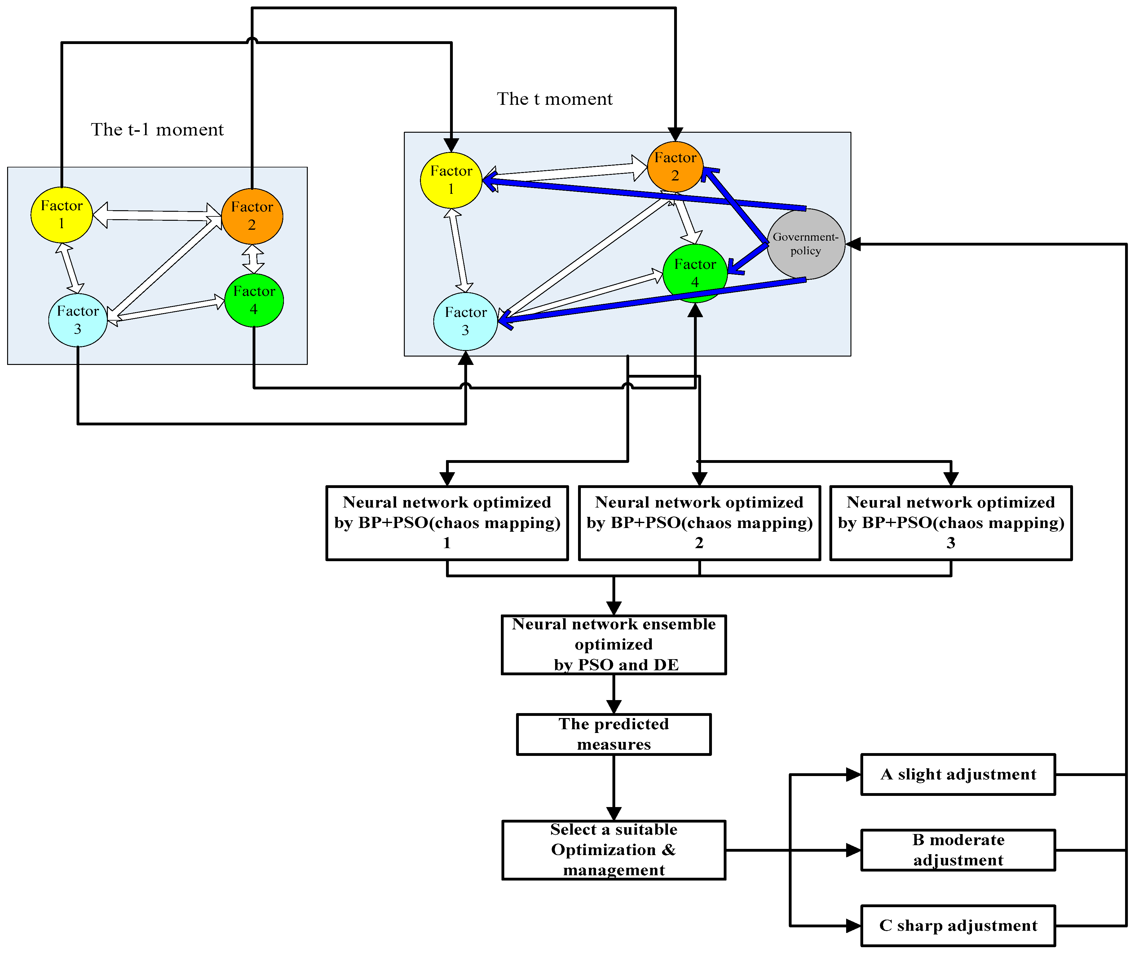
Our model is composed of three segments: the first estimates the global dynamic influence of factors via the local interacting factors. The second predicts the measured values for the ecosystem that could reflect the whole ecosystem’s state. The third determines the critical factors and loop control to adjust the ecosystem. In
Figure 1, we present the schematic diagram as follows.
In the colorful block, the white double arrow denotes the interacting influence between two local factors. From t − 1 moment to t moment, it is a dynamic alignment that incorporates the Markov property. The flow arrows mean the prediction of the neural networks. A, B, and C denote the different government policies. The blue single side arrow denotes the policy acting on the input factors. The feedback circle means that the government takes measures to tackle the global state change.
3. Model Solution
3.1. Estimating the Dynamic Factors
In the first sub-section, we presented the Markov chain to reflect the influence between the
t moment and
t − 1 moment. We assumed that the
k –
th factor at the
t moment is influenced by the same factor at the
t − 1 moment and the interacting factors in neighborhood at the
t moment, and ignore the influence between different factors at the
t − 1 moment, which is reasonable in order to simplify the model by the Markov property. Thus we could construct an estimation matrix M that incorporates the interactive relationship of different dynamic factors. In
Table 2, we list the estimated Markov impacting matrix M.
The elements in the leading diagonal denote a continuous effects on the same factor over time (t − 1 & t). The other elements in the matrix present the effect on different factors at the same t moment. The difference between the k – th factor and the m – th factor reflects on characteristic variations of industrial and agricultural production, consumption, and populations at the same time period.
We could obtain the estimated dynamic factors using the following formula:
We regard as the dynamic factors of the Neural Network Ensemble (NNE). Via all these input factors above, we could predict the output measure.
3.2. Predicting the Output Measure
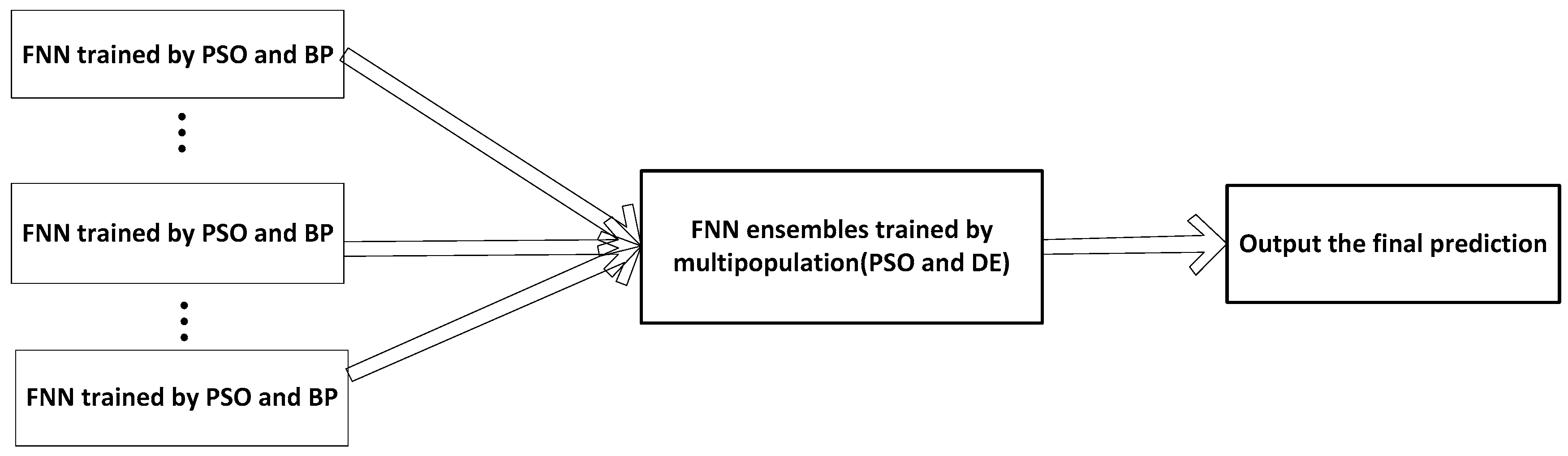
Having obtained the estimated dynamic factors, the output measure of the ecological modeling can be predicted using our previously proposed Evolved Neural Network Ensemble (NNE), improved by Multiple Heterogeneous Swarm Intelligence [
9]. Compared to the ordinary NNE, to improve the prediction precision, we incorporate the Particle Swarm Optimization (PSO) [
10,
11] and Back Propagation (BP) algorithms to train each component Forward Neural Network (FNN). Meanwhile, we apply logistic chaos mapping to enhance the local searching ability. At the same time, the ensemble weights are trained by multi-population algorithms (PSO and Differential Evolution (DE) [
9] cooperative algorithms are used in this case). By the NNE algorithms, we could remove the disturbance in the data. A more detailed description is given in [
9]. In
Figure 2, we summarize the schematic diagram of the improved NNE as follows:
We could divide this sub-section into two parts: one is how to train and optimize the component neural networks; the other is how to optimize the NNE by multi-population algorithms.
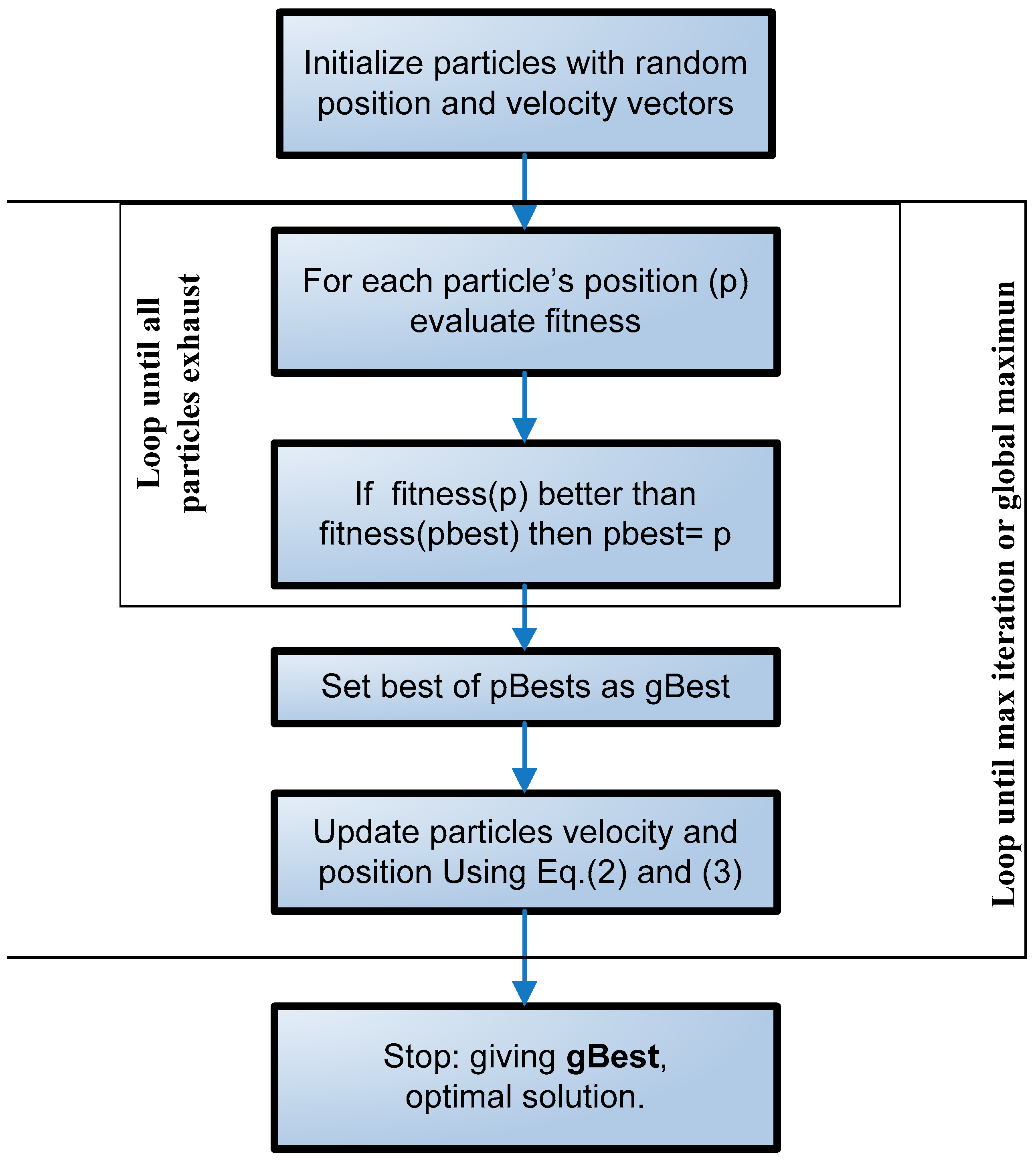
3.2.1. Optimization by Particle Swarm Optimization (PSO) Algorithm, Chaotic Mapping, and Back Propagation (BP) Algorithm
The PSO could be described as a swarm of birds hovering in the sky for food.
Xi = (
xi1,
xi2, …,
xin) and
Vi = (
vi1,
vi2, …,
vin), where
Xi and
Vi are the position and velocity of the
i –
th particle in
n dimensional space.
Pi = (
pi1,
pi2,… ,
pin) represents the previous best value of the
i –
th particle up to the current step.
Gi = (
gi1,
gi2,… ,
gin) represents the best value of all particles in the population. Having obtained the two best values, each particle updates its position and velocity according to the following equations:
c1 and
c2 are learning actors.
wt is the inertial weight. The flow chart depicting the general PSO Algorithm is given in
Figure 3. A more detailed description is given in [
9,
10,
11].
In addition, with the purpose of enhancing the local searching ability and diversity of the particle swarm, we incorporate the chaos mechanism [
12] into the updating iteration. We take the logistic mapping as the chaos producer.
The well-known idea of BP is to make the error back propagate to update the parameters of FNN, and the parameters include two steps: one is between the input layer and hidden layer; the other is between the hidden layer and the output layer.
A detailed description of the procedures of the PSO (combined logistic mapping)–BP coupled algorithm is presented is in [
9,
10].
3.2.2. Optimization by Multi-Population Cooperative Algorithm
The principle of the NNE has been described in detail in [
9,
13,
14]. Having obtained each refined component FNN, we would concentrate on how to combine the output of each component FNN.
where
fi (
x) represents the output of the
i –
th FNN and
represents the importance of the
i –
th FNN. Our idea is to obtain the most appropriate prediction of
for each sub-network, which corresponds to the solution of the optimization problem of the particles. DE is also a floating, point-encoded evolutionary algorithm for global optimization over continuous spaces, but it creates new candidate solutions by combining the parent individual and several other individuals of the same population. It consists of selection, crossover, and mutation [
15].
The procedure for NNE multi-population algorithm could be summarized as follows:
Step 1: Initialize the weight of each FNN, which has been optimized by PSO (combined logistic mapping) and BP.
Step 2: Each particle represents a set of weights, which means that each dimension represents one weight of each component FNN. The population is duplicated into two identical swarms.
Step 3: One swarm is optimized by PSO and the other is optimized by DE.
Step 4: Update the gbest_PSO and gbest_DE.
Step 5: Do the Steps 3–4 loop until the Max-iteration is reached.
Step 6: Output the predicted measures.
3.3. Optimization and Management
In the third sub-section, we could determine the critical factors by sensitivity analysis and determine the measurement standards that could evaluate the state change. The local state change could influence the global state and vice versa. Via a different management mechanism, government policy could be established and the ecosystem could be developed according to the sustainable direction.
3.3.1. Sensitivity Design
Having obtained the dynamic predicted measures, we could calculate the sensitivity between the input factors and the predicted measures.
We determined
, which denotes a change of input or output state, and obtained the values using the following formulae:
We could calculate the sensitivity between the predicted measure and the estimated input factors using the following formula:
, which could take the approximated format:
We would get the following results:
If , it denotes a negative influence. The predicted measures would decrease, with the input factor increasing.
If , it means a positive influence. With the input factor increasing, the predicted measures would increase.
The bigger the absolute value of is, the more powerful the influence between the input factor and the predicted measures would be. By this means we could obtain the critical factor, which acts on the global influence.
3.3.2. Management and Policy
We take the fuzzy rules to determine the measure standard, and we also take the last 5th year as the comparison. With several values as thresholds, the rules can be described as follows:
If , it means that the state has changed slightly. We could adopt policy A, which acts on the critical factor of .
Otherwise, if , it means that the state has changed moderately.
Alternatively, we could adopt policy B, which acts on the critical factor of .
Otherwise, if , it means that the state has seriously changed.
Lastly, we could adopt policy C, which acts on the critical factor of .
End If.
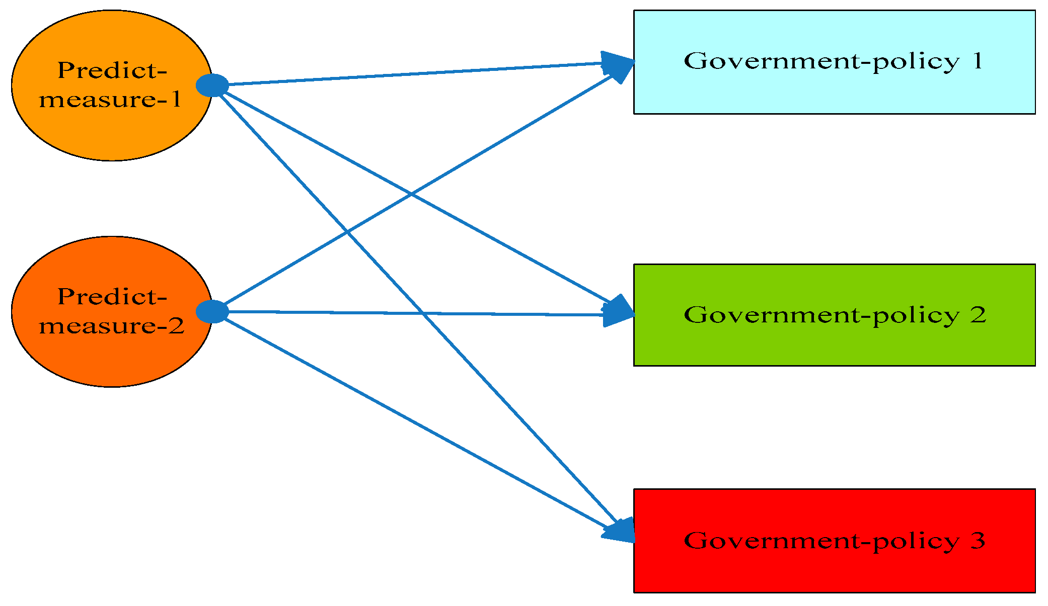
In
Figure 4, we present the management diagram as follows:
We choose the suitable policy to control the critical factor of each predicted value. We also make a rule table as follows. By this means we could obtain a suitable policy for overall prediction of
. In
Table 3, we give the rules table.
We could make a brief policy mechanism with the pseudo-code description given in
Table 4.
Based on the predicted measures, we could suggest that the government draft detailed policies. For example:
Policy A: Increase public awareness of (1) the damage caused by increasing CO2; (2) the damage caused by logging; (3) the dangers linked to an increasing population; and (4) strategies for economizing on electricity.
Policy B: Limit (1) car exhaust; (2) large-scale logging; (3) population by slight measures; (4) electrical consumption in certain areas or certain time periods; and (5) develop novel technologies to tackle the problem.
Policy C: (1) Make laws to limit CO2 and fuel consumption and (2) advocate forest planting.
4. Data Testing and Analysis
4.1. Data Design
The dataset for ecological modeling is collected from references [
8,
16,
17,
18] (unfortunately, we cannot access all the fields of the dataset for 2007–2015). The local factor data and the real measured data are shown in the
Table 5 and
Table 6, respectively.
Factors such as CO2 content, oil consumption, population, and power consumption are regarded as the input factors. Using the Markov estimation, we could get the estimated input factors.
4.2. Training and Analysis
We adopt the data from 1996 to 2001 to train our neural networks. The input variables include CO
2, oil consumption, population, and power consumption, and the predicted measures include the morbidity rate and GDP. A sensitivity analysis is conducted to determine the critical factors and put forward advice that would help the government to establish policy. In
Table 7, we list the sensitivity of the input factors and predicted measures from 1997 to 2001.
From
Table 7, we could draw a conclusion that the CO
2 content has been the critical factor. In our model, CO
2 stands for the environmental change.
In 1997, CO2 was the main factor behind the rapid increase of GDP, and also strengthened the morbidity rate. This means that the GDP increasing is based on environmental deterioration. Meanwhile, the deteriorating environment has caused an increase in the morbidity rate.
From 1998 to 1999, CO2 has also been the prominent factor in the rapid increasing of GDP, and exacerbated the morbidity rate. However, the increase has plateaued, which means that the government has recognized the problem and taken slight measures to tackle it.
In 2000, CO2 shifted from a positive role to a negative factor in relation to the morbidity rate, but meanwhile it strengthened the GDP. This means that the government has taken measures to prevent some diseases. However, GDP increasing is also based on environmental deterioration.
In 2001, CO2 was a negative factor in relation to the GDP and morbidity rate. By a sensitivity analysis of morbidity rate, we found that environmental deterioration has alleviated the positive influence of the government policies that prevent some diseases. Even more, the environmental deterioration has hindered the increasing of GDP.
4.3. Testing and Analysis
We use data from 2001–2006 to test our model. We could draw the conclusion that our model could fit the approximating trend of the two predicted measures. In
Table 8, we list the sensitivity of the input factors and predicted measures from 2002 to 2006.
From
Table 8, we could draw a conclusion that in 2002–2003 the oil consumption was the critical factor and in 2004–2006 CO
2 content was the critical factor. In our model, CO
2 denotes environmental change and oil consumption could represent resource consumption.
In 2002, oil consumption was a positive factor in relation to the rapid increasing of GDP, but strengthened the morbidity rate. In the last five years, the government has adopted several policies to tackle environmental deterioration. However, it must be noticed that GDP increasing is also based on resource consumption. In the meantime, excessive resource consumption has brought about an increase in the morbidity rate. The system must be monitored for both intended and unintended changes. The government should take measures to optimize the resource consumption mechanism.
Compared with the sensitivity of 2002, we could see that excessive resource consumption has further strengthened the morbidity rate, and also limited the increase of GDP. However, by 2002, the government had not taken effective measures.
In 2004–2006, the morbidity rate was alleviated by government policy. The GDP improved from 2004 to 2006. The government adopted some beneficial environmental policies but, over time, overconsumption of resources always negatively affects the environment. For some accumulated reasons, the CO2 content could not be decreased but could be controlled to some extent.
5. Conclusions and Discussion
Our predictive model could fit the real trends. It could be an effective method to reflect the relationship between input factors and predicted measurements; in addition, the model helps to determine critical factors and measurement standards. By referring to this model, the government could make a detailed policy for adjusting the ecosystem. However, it must be noticed that when a large number of factors are considered, we have to construct a complicated matrix to reflect the dynamic relationship; so the simulation would be heavy, so a prominent component analysis would be considered.
Our method has the following strengths:
Firstly, our model can incorporate the relationships between different local state factors, taking into account different changing variables.
Secondly, the Neural Network Ensemble (NNE) is used to predict the global state. The predicting of single neural networks would be sensitive to disturbance. However, NNE could improve the stability of the model. In addition, PSO with logistic chaotic mapping could optimize the parameters in the networks and improve precision. The multi-population cooperative algorithm could enhance the stability of the NNE.
Lastly, by the analysis of sensitivity, our model could confirm the critical factors that affect the global state. Moreover, our model could determine the measurement standards used to select a policy.
Acknowledgments
This work was supported in part by the National Natural Science Foundation of China (Grant No. 61403281), the Natural Science Foundation of Shandong Province (ZR2014FM002), and a China Postdoctoral Science Special Foundation Funded Project (2015T80717).
Author Contributions
Rong Shan wrote the source code, revised the article; Zeng-Shun Zhao designed the algorithm, wrote the manuscript, analysed and interpretated the data; Pan-Fei Chen and Wei-Jian Liu conceived and designed the experiments; Shu-Yi Xiao and Yu-Han Hou performed the experiments; Mao-Yong Cao, Fa-Liang Chang and Zhigang Wang analyzed the data.
Conflicts of Interest
The authors declare no conflict of interest.
References
- Barnosky, A.D.; Hadly, E.A.; Bascompte, J.; Berlow, E.L.; Brown, J.H.; Fortelius, M.; Getz, W.M.; Harte, J.; Hastings, A.; Marquet, P.A.; et al. Approaching a state shift in Earth’s biosphere. Nature 2012, 486. [Google Scholar] [CrossRef] [PubMed]
- Mills, J.I.; Emmi, P.C. Limits to growth: The 30-year update. J. Policy Anal. Manag. 2006, 25, 241–245. [Google Scholar] [CrossRef]
- Scheffer, M.; Bascompte, J.; Brock, W.A.; Brovkin, V.; Carpenter, S.R.; Dakos, V.; Held, H.; van Nes, E.H.; Rietkerk, M.; Sugihara, G. Early-warning signals for critical transitions. Nature 2009, 461, 53–59. [Google Scholar] [CrossRef] [PubMed]
- Drake, J.M.; Griffen, B.D. Early warning signals of extinction in deteriorating environments. Nature 2010, 467, 456–459. [Google Scholar] [CrossRef] [PubMed]
- Brown, J.H.; Burnside, W.R.; Davidson, A.D.; DeLong, J.P.; Dunn, W.C.; Hamilton, M.J.; Mercado-Silva, N.; Nekola, J.C.; Okie, J.G.; Woodruff, W.H.; et al. Energetic limits to economic growth. Bioscience 2011, 61, 19–26. [Google Scholar] [CrossRef]
- McDaniel, C.N.; Borton, D.N. Increased human energy use causes biological diversity loss and undermines prospects for sustainability. Bioscience 2002, 52, 929–936. [Google Scholar] [CrossRef]
- Maurer, B.A. Relating human population growth to the loss of biodiversity. Biodivers. Lett. 1996, 3, 1–5. [Google Scholar] [CrossRef]
- Lavergne, S.; Mouquet, N.; Thuiller, W.; Ronce, O. Biodiversity and climate change: Integrating evolutionary and ecological responses of species and communities. Annu. Rev. Ecol. Evol. Syst. 2010, 41, 321–350. [Google Scholar] [CrossRef]
- Zhao, Z.; Feng, X.; Lin, Y.; Wei, F.; Wang, S.; Xiao, T.; Cao, M.; Hou, Z. Evolved neural network ensemble by multiple heterogeneous swarm intelligence. Neuro Comput. 2015, 149, 29–38. [Google Scholar] [CrossRef]
- Zhao, Z.; Feng, X.; Lin, Y.; Wei, F.; Wang, S.; Xiao, T.; Cao, M.; Hou, Z.; Tan, M. Improved Rao-Blackwellized particle filter by particle swarm optimization. J. Appl. Math. 2013, 2013, 1–7. [Google Scholar] [CrossRef]
- Kennedy, J.; Eberhart, R. Particle Swarm Optimization. In Proceedings of the IEEE Conference on Neural Networks, Piscataway, NJ, USA, 27 November 1995; pp. 1942–1948.
- Gulick, D. Encounters with Chaos; McGraw Hill, Inc.: New York, NY, USA, 1992; pp. 127–186, 195–220, 240–285. [Google Scholar]
- Optiz, D.; Shavlik, J. Actively searching for an effectively neural network ensemble. Connect. Sci. 1996, 8, 337–353. [Google Scholar] [CrossRef]
- Valentini, G.; Masulli, F. Ensembles of learning machines. WIRN VIETRI 2002, 2002, 3–20. [Google Scholar]
- Storn, R.; Price, K. Differential evolution—A simple and efficient heuristic for global optimization over continuous spaces. J. Glob. Optim. 1997, 11, 341–359. [Google Scholar] [CrossRef]
- Data-The World Bank. Available online: http://data.worldbank.org.cn/ (accessed on 12 December 2015).
- US-The Census Bureau. Available online: http://www.census.gov/compendia/statab/cats/births_deaths_marriages_divorces.html (accessed on 12 December 2015).
- Population-Polution. Available online: http://www.google.com.hk/publicdata/explore?ds=d5bncppjof8f9_&met_y=sp_pop_totl&tdim=true&dl=zh-CN&hl=zh-CN&q=%E5%85%A8%E7%90%83%E4%BA%BA%E5%8F%A3 (accessed on 20 November 2015).
© 2016 by the authors; licensee MDPI, Basel, Switzerland. This article is an open access article distributed under the terms and conditions of the Creative Commons Attribution (CC-BY) license (http://creativecommons.org/licenses/by/4.0/).


