Article

Novel Graphical Representation and Numerical Characterization of DNA Sequences

1
Department of Mathematics, Bohai University, Jinzhou 121013, China
2
Research Institute of Food Science, Bohai University, Jinzhou 121013, China
3
Department of Applied Mathematics, Shanghai Institute of Technology, Shanghai 201418, China
*
Author to whom correspondence should be addressed.
Appl. Sci. 2016, 6(3), 63; https://doi.org/10.3390/app6030063
Submission received: 10 December 2015 / Revised: 5 February 2016 / Accepted: 14 February 2016 / Published: 24 February 2016
(This article belongs to the Special Issue Dynamical Models of Biology and Medicine)

Abstract

:
Modern sequencing technique has provided a wealth of data on DNA sequences, which has made the analysis and comparison of sequences a very important but difficult task. In this paper, by regarding the dinucleotide as a 2-combination of the multiset { · A , · G , · C , · T } , a novel 3-D graphical representation of a DNA sequence is proposed, and its projections on planes (x,y), (y,z) and (x,z) are also discussed. In addition, based on the idea of “piecewise function”, a cell-based descriptor vector is constructed to numerically characterize the DNA sequence. The utility of our approach is illustrated by the examination of phylogenetic analysis on four datasets.

Graphical Abstract

1. Introduction

The rapid development of DNA sequencing techniques has resulted in explosive growth in the number of DNA primary sequences, and the analysis and comparison of biological sequences has become a topic of considerable interest in Computational Biology and Bioinformatics. The traditional measure for similarity analysis of DNA sequences is based on multiple sequence alignment, which uses dynamic programming techniques to identify the globally optimal alignment solution. However, the sequence alignment problem is NP-hard (non-deterministic polynomial-time hard), making it infeasible for dealing with large datasets [1]. To overcome the limitation, a lot of alignment-free approaches for sequence comparison have been proposed.
The basic idea behind most alignment-free methods is to characterize DNA by certain mathematical models derived for DNA sequence, rather than by a direct comparison of DNA sequences themselves. Graphical representation is deemed to be a simple and powerful tool for the visualization and analysis of bio-sequences. The earliest attempts at the graphical representation of DNA sequences were made by Hamori and Ruskin in 1983 [2]. Afterwards, a number of graphical representations were well developed by researchers. For instance, by assigning four directions defined by the positive/negative x and y coordinate axes to the four nucleic acid bases, Gates [3], Nandy [4,5], and Leong and Morgenthaler [6] introduced three different 2-D graphical representations, respectively. While Jeffrey [7] proposed a chaos game representation (CGR) of DNA sequences, in which the four corners of a selected square are associated with the four bases respectively. In 2000, Randic et al. [8] generalized these 2-D graphical representations to a 3-D graphical representation, in which the center of a cube is chosen as the origin of the Cartesian (x,y,z) coordinate system, and the four corners with coordinates (+1,−1,−1), (−1,+1,−1), (−1,−1,+1), and (+1,+1,+1) are assigned to the four bases. Some other graphical representations of bio-sequences and their applications in the field of biological science and technology can be found in [9,10,11,12,13,14,15,16,17,18,19,20,21,22,23,24].
Numerical characterization is another useful tool for sequence comparison. One way to arrive at the numerical characterization of a DNA sequence is to associate the sequence with a vector whose components are related to k-words, including the single nucleotide, dinucleotide, trinucleotide, and so on [25,26,27,28,29,30]. In addition, the numerical characterization can be accomplished by associating with a graphical representation given by a curve in the space (or a plane) structural matrices, such as the Euclidean-distance matrix (ED), the graph theoretical distance matrix (GD), the quotient matrix (D/D, M/M, L/L), and their “higher order” matrices [8,9,10,11,12,13,14,15,16,17,18,31,32,33]. Once a matrix representation of a DNA sequence is given, some matrix invariants, e.g. the leading eigenvalues, can be used as descriptors of the sequence. This technique has been widely used in the field of biological science and medicine, and different types of matrices are defined to construct various invariants of DNA sequences. However, the order of these matrices is equal to n, the length of the DNA sequence considered. A problem we must face is that the calculation of these matrix invariants will become more and more difficult with larger n values [17,24,32].
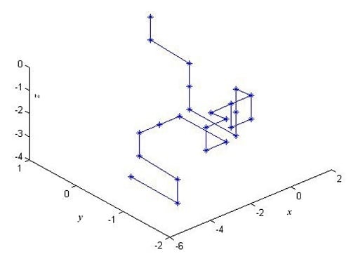
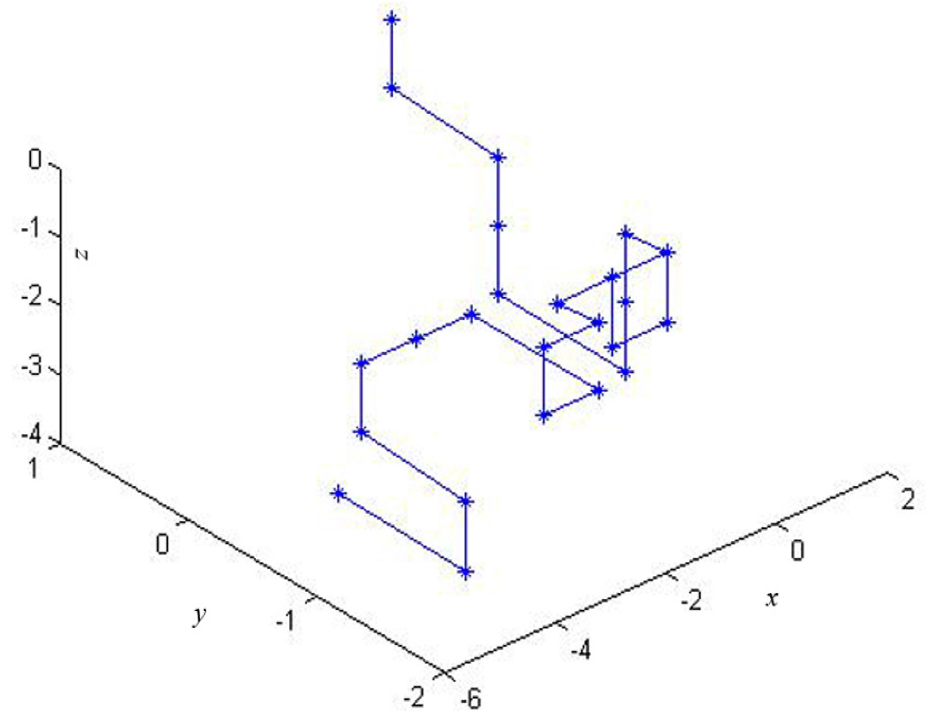
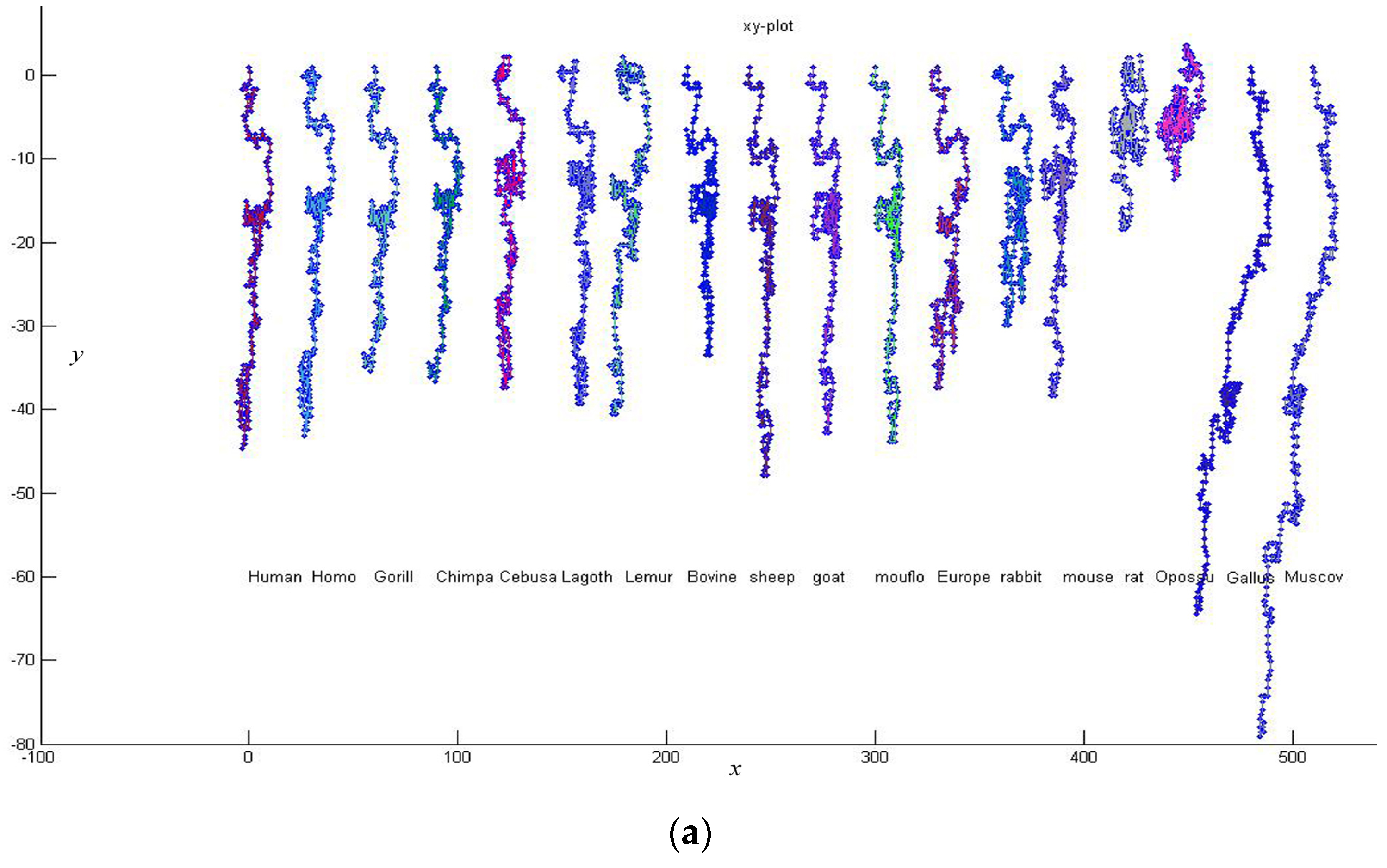
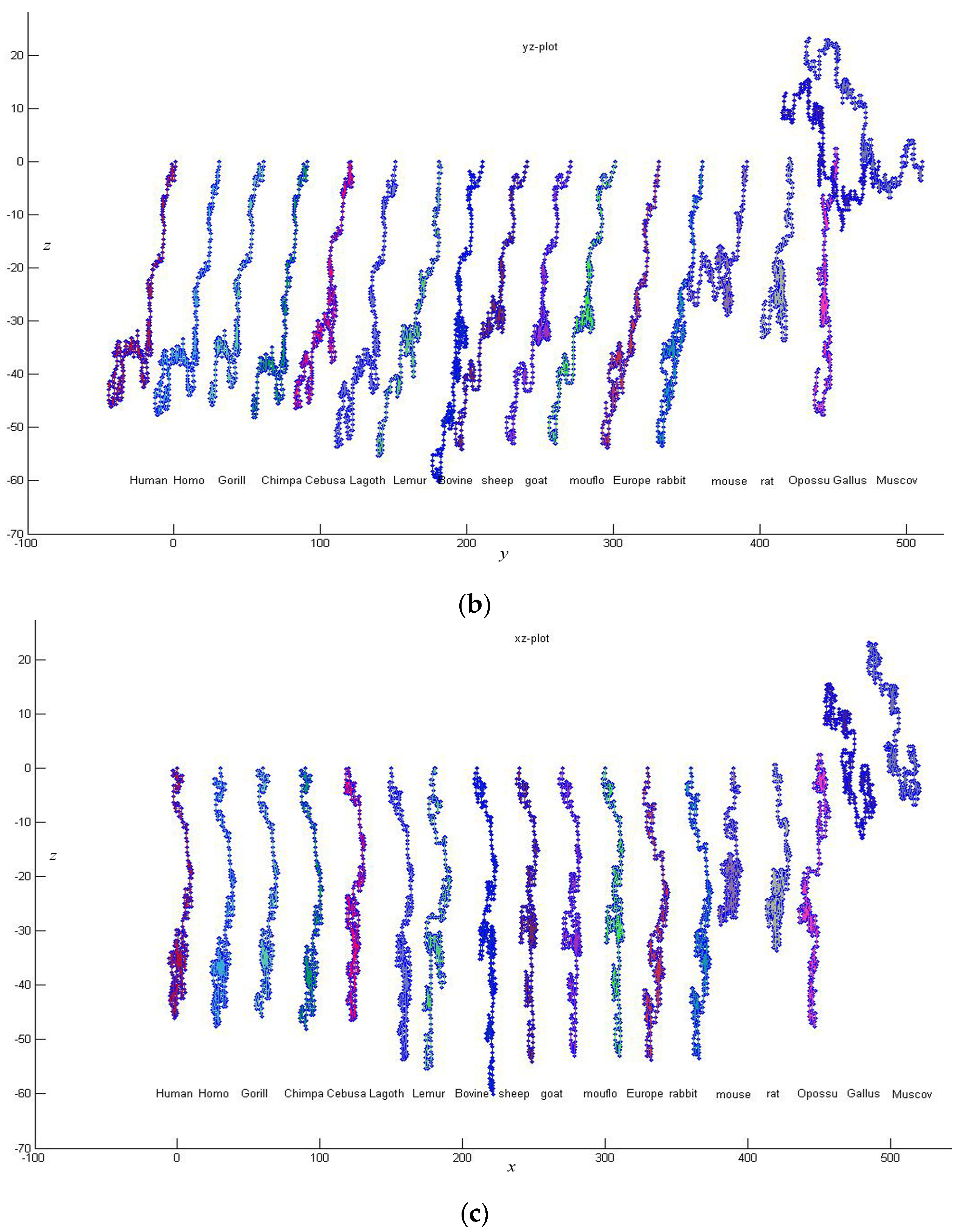
In this paper, based on all of the 2-combinations of the multiset { · A , · G , · C , · T } , we propose a novel graphical representation of DNA sequences. Then, according to the idea of “piecewise function”, we describe a particular scheme that transforms the graphical representation of DNA into a cell-based descriptor vector. The introduced vector leads to more simple characterizations and comparisons of DNA sequences.

2. Methods

2.1. The 3-D Graphical Representation

As we know, the four nucleic acid bases A, G, C, and T can be classified into three categories:
R = {A,G}/Y = {C,T}; M = {A,C}/K = {G,T}; W = {A,T}/S = {G,C}.
In fact, these groups are just all of the non-repetition 2-combinations of set {A,G,C,T}. If repetition is allowed, in other words, if we consider multiset { · A , · G , · C , · T } instead of the set {A,G,C,T}, then the number of 2-combinations equals 10 (see Table 1).
Let V be a regular tetrahedron whose center is at the origin O = ( 0 , 0 , 0 ) . V 1 = (+1,+1,+1), V 2 = (−1,−1,+1), V 3 = (+1,−1,−1), and V 4 = (−1,+1,−1) are its four vertices. To each of the vertices we assign one of the four nucleic acid bases A, C, G and T. Moreover, to the midpoint of the line segment AC we assign M, and K to the midpoint of the line segment GT, R to that of the line segment AG, Y to that of the line segment CT, W to that of the line segment AT, and S to that of the line segment CG. We thus obtain ten fixed directions: O A , O C , O G , O T , O M , O K , O R , O Y , O W , O S , based on which we can derive ten unit vectors:
r A = 1 O A O A ,   r C = 1 O C O C , ,   r S = 1 O S O S
Obviously, the ten unit vectors are ten points on a unit sphere.
An idea arises naturally: each of the ten 2-combinations can be associated with one of the ten unit vectors. In detail, we have
{ A , A } r A ,   { A , G } r R ,   { A , C } r M , { A , T } r W , { G , G } r G , { G , C } r S , { G , T } r K , { C , C } r C ,   { C , T } r Y ,   { T , T } r T .
To obtain the spatial curve of a DNA sequence, we move a unit length in the direction that the above assignment dictates. Taking sequence segment ATGGTGCACCTGACTCCTGATCTGGTA as an example, we inspect it by stepping two nucleotides at a time. Starting from the origin O = ( 0 , 0 , 0 ) , we move in the direction dictated by the first dinucleotide AT, r W , and arrive at P 1 , the first point of the 3-D curve. From this point, we move in the direction dictated by the second dinucleotide TG, r K , and arrive at the second point P 2 . From here we move in the direction dictated by the third dinucleotide GG, r G , and come to the third point P 3 . Continuation of this process is illustrated in Table 2, and the corresponding 3-D graphical representation is shown in Figure 1.
As the characterization of a research object, a good visualization representation should allow us to see a pattern that may be difficult or impossible to see when the same data is presented in its original form. In order to provide a direct insight into the local and global characteristics of a DNA sequence, the proposed 3-D curve can be projected on planes (x,y), (y,z) or (x,z), and thus three different 2-D graphical representations will be yielded. Figure 2 shows the projections of 3-D curves of 18 different DNA sequences listed in Table 3.
It is easy to see that, in each projection, the trend of curves of the two non-mammals (Gallus, Muscovy duck) is distinguished from that of the mammals. On the other hand, the Primates species are similar to one another, so it is with the curves of bovine, sheep, goat, and mouflon. Also, the curves of rabbit and European hare show their great similarity. In addition, both Figure 2b, the projection on yz-plane, and Figure 2c, the projection on xz-plane, show opossum has relatively low similarity with the remaining mammals, while mouse and rat look similar to each other because both of their curves wind themselves into a mass and need a relatively small space.

2.2. Numerical Characterization of DNA Sequences

The graphical representations not only offer the visual inspection of data, helping in recognizing major differences among DNA sequences, but also provide with the numerical characterization that facilitates quantitative comparisons of DNA sequences. One way to arrive at the numerical characterization of a DNA sequence is to convert its graphical representation into some structural matrices, and use matrix invariants, e.g., the leading eigenvalues, as descriptors of the DNA sequence [8,9,10,11,12,13,14,15,16,17,18,31,32]. It is expected that effective invariants will emerge and enable to uniquely characterize the sequences considered. However, the difficulties associated with computing various parameters for very large matrices that are natural for long sequences have restricted the numerical characterizations, for instance, leading eigenvalues and the like [17,24]. The search for novel descriptors may be an endless project. The art is in finding useful descriptors, and those that have plausible structural interpretation, at least within the model considered [8]. In this section, we bypass the difficulty of calculating the invariants like the leading eigenvalue and propose a novel descriptor to numerically characterize a DNA sequence.
As described above, the pattern, including shape and trend, of curves for the 18 DNA sequences provides useful information in an efficient way. This inspires us to numerically characterize a DNA sequence with an idea of “piecewise function” as below.
For a given 3-D graphical representation with n vertices, by the order in which these vertices appear in the curve, we partition it into K parts, each of which is called a cell. All the cells contain m = n K vertices except the last one. For the i-th cell, i = 1,2,...,K, the geometric center U i = ( x i , y i , z i ) is viewed as its respective. Then we have
U i 1 U i = ( x i x i 1 , y i y i 1 , z i z i 1 )
where U 0 = ( 0 , 0 , 0 ) . It is not difficult to find that U i 1 U i reflects a certain “growing trend” of these cells. For convenience, we call U i 1 U i the trend-point. On the basis of the K trend-points, a DNA sequence can be characterized by a 3K-dimensional vector V t p :
V t p = ( x 1 x 0 , x 2 x 1 , , x k x k 1 , y 1 y 0 , y 2 y 1 , , y k y k 1 , z 1 z 0 , z 2 z 1 , , z k z k 1 )
In this paper, K is determined by r o u n d ( log 4 L ¯ 2 2 ) , where L ¯ = 1 N j = 1 N | s j | , N is the cardinality of the dataset Ω considered, and | s j | stands for the length of sequence s j Ω . Taking for example the two non-mammals of the 18 species, the corresponding vectors can be calculated as
V Gallus = ( 4.524 , 9.588 , 5.546 , 10.962 , 9.234 , 20.304 , 9.824 , 12.093 , 4.087 , 0.450 , 10.255 , 5.615 ) ,
V MDuck = ( 6.186 , 10.593 , 3.440 , 12.511 , 10.639 , 21.519 , 12.987 , 18.351 , 1.244 , 0.498 , 10.478 , 9.325 ) .

3. Results and Discussion

In this section, we will illustrate the use of the proposed cell-based descriptor V t p of a DNA sequence. For any two sequences S a and S b , suppose their descriptor vectors are a = ( a 1 , a 2 , , a 3 k ) and b = ( b 1 , b 2 , , b 3 k ) , respectively. Then, their similarity can be examined by the following Euclidean distance. Clearly, the smaller the Euclidean distance is, the more similar the two DNA sequences are.
d ( a , b ) = j = 1 3 k ( a j b j ) 2
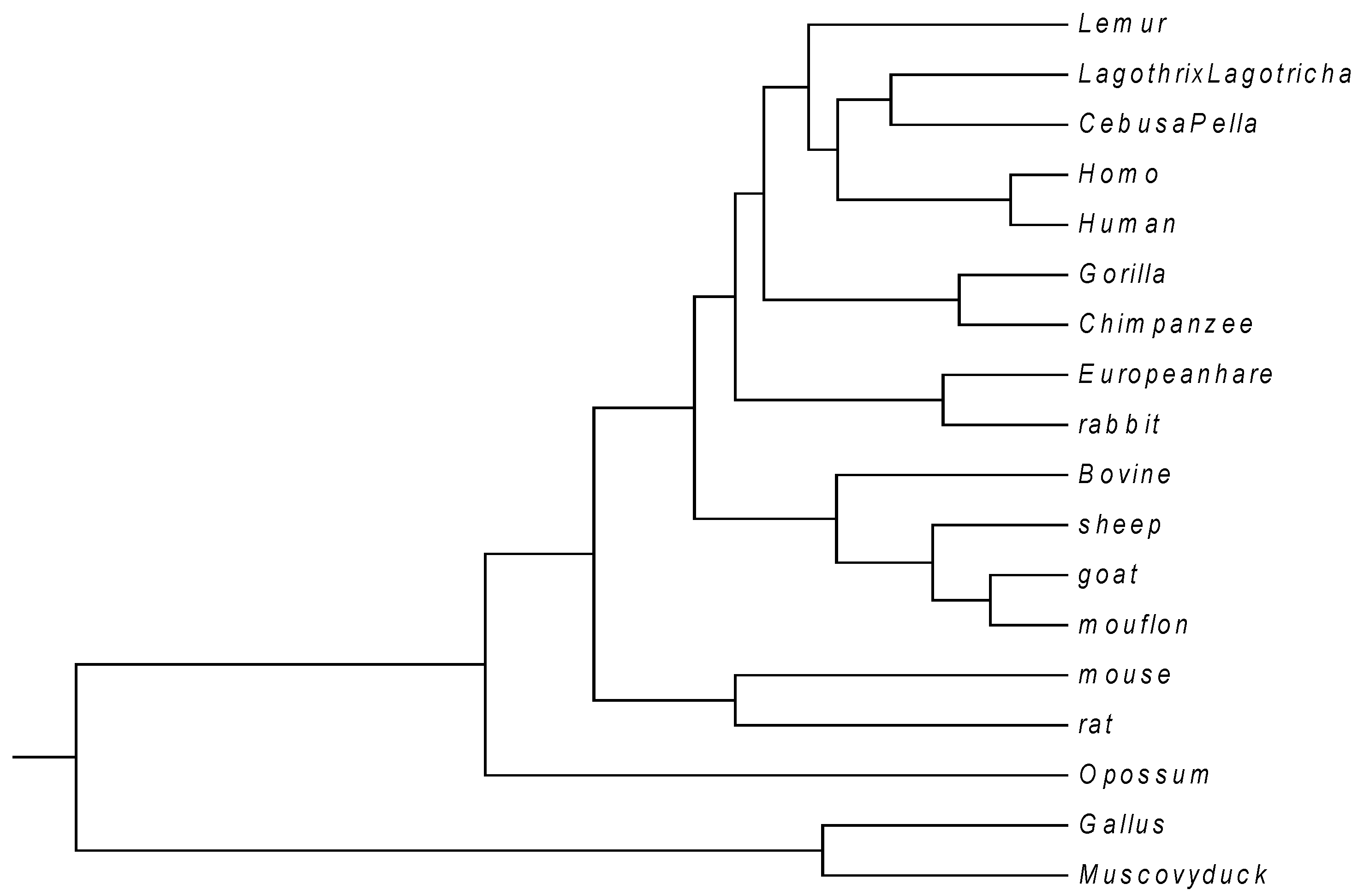
Firstly, we give a comparison for CDS (Coding DNA Sequence) of β-globin gene of 18 species listed in Table 3. The lengths of the 18 sequences are about 434 bp. Thus K is taken to be 4, and each of these sequences is converted into a 12-D vector. According to Equation (7), we calculate the distance between any two of the 18 DNA sequences. Then an 18 × 18 real symmetric matrix D 18 is obtained. On the basis of D 18 , a phylogenetic tree (see Figure 3) is constructed using UPGMA (Unweighted Pair Group Method with Arithmetic Mean) program included in MEGA4 [34]. Observing Figure 3, we find that the CDS are more similar for Primate group {Gorilla, Chimpanzee, Human, Homo, CebusaPella, LagothrixLagotricha, Lemur}, Cetartiodactyla group {bovine, sheep, goat, mouflon}, Lagomorpha group {Rabbit, European hare}, and Rodentia group {mouse, rat}, respectively. On the other hand, CDS of the two kinds of non-mammals {Gallus, Muscovy duck} are very dissimilar to the mammals because they are grouped into an independent branch. This is analogous to that reported in the literature [8,12,14,31], and the relationship of these species detected by their graphical representations as well. From this result, a conclusion one can draw is that the cell-based descriptors of the new graphical representation may suffice to characterize DNA sequences.
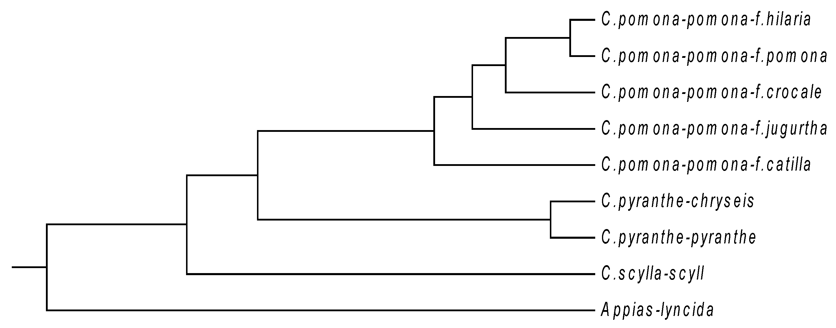
In order to further illustrate the effectiveness of our method, we test it by phylogenetic analysis on other three datasets: one consists of mitochondrial cytochrome oxidase subunit I (COI) genes of nine butterflies, another includes S segments of 32 hantaviruses (HVs), and the last is composed of 70 complete mitogenomes (mitochondrial genomes). For convenience, we denote the three datasets by COI, HV and mitogenome, respectively. In the COI dataset (see Table 4), which is taken from Yang et al. [12], eight belong to the Catopsilia genus and one belongs to Appias genus, which is used as the out-group. The average length of these COI gene sequences is 661 bp, and thus K, the number of cells, is calculated as 4. According to the method mentioned above, a distance matrix is constructed, and then a phylogenetic tree (see Figure 4) is generated. Figure 4 shows that the five pomona sub-species have relatively high similarity with each other, while the two pyranthe sub-species cluster together. In addition, scylla sub-species is situated at an independent branch, whereas the Appias lyncida stays outside of all the Catopsilia. This result is consistent with that reported in [12,35].
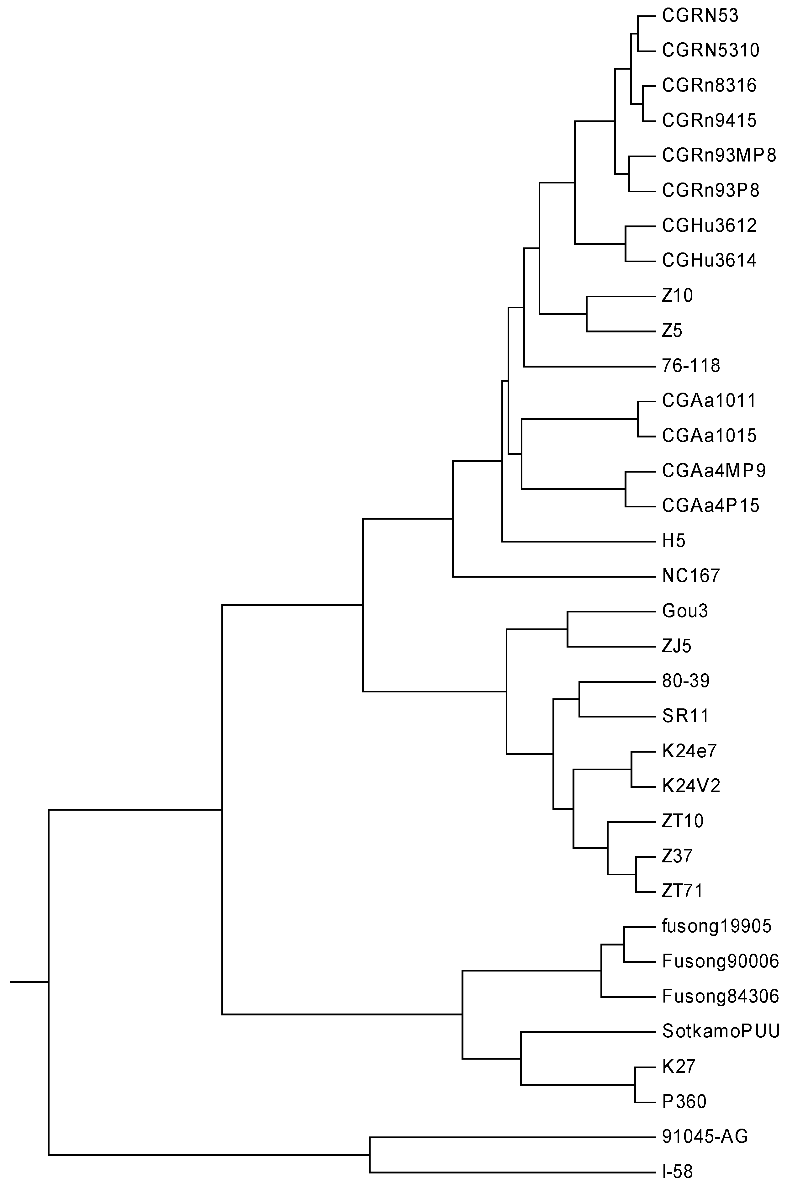
The hantavirus (HV), which is named for the Hantan River area in South Korea, is a relatively newly discovered RNA virus in the family Bunyaviridae. This kind of virus normally infects rodents and does not cause disease in these hosts. Humans may be infected with HV, and some HV strains could cause severe, sometimes fatal, diseases in humans, such as HFRS (hantavirus hemorrhagic fever with renal syndrome) and HPS (hantavirus pulmonary syndrome). The later occurred in North and South America, while the former mainly in Eurasia [12,36]. In Eastern Asia, particularly in China and Korea, the viruses that cause HFRS mainly include Hantaan (HTN) and Seoul (SEO) viruses, while Puumala (PUU) virus is found in Western Europe, Russia and northeastern China. The HV dataset analyzed in this paper includes 32 HV sequences. Phlebovirus (PV) is another genus of the family Bunyaviridae. Here, two PV strains KF297911 and KF297914 are used as the out-group. The name, accession number, type, and region of the 34 sequences are described in Table 5. The lengths of these sequences are in the range of 1.30–1.88 kbp. Thus K is calculated as 5, and each of the 34 viruses is converted into a 15-D vector. The phylogenetic tree constructed by our method is shown in Figure 5.
From Figure 5, we find that the two PV strains form an independent branch, which can be distinguished easily from the HV strains, while the 32 HVs are grouped into three separate branches: the strains belonging to PUUV are clearly clustered together, the strains belonging to SEOV appear to cluster together, and so do the ones belonging to HTNV. A closer look at the subtree of HTNV, all CGRn strains whose host is Rattus norvegicus tend to cluster together, so it is with the CGHu strains whose host is Homo sapiens. In addition, all the four CGAa strains whose host is Apodemus agrarius are grouped closely. Needless to say, the phylogeny is not only closely related to the isolated regions, but also has certain relationship with the host. This result is similar to that reported in [12,37].
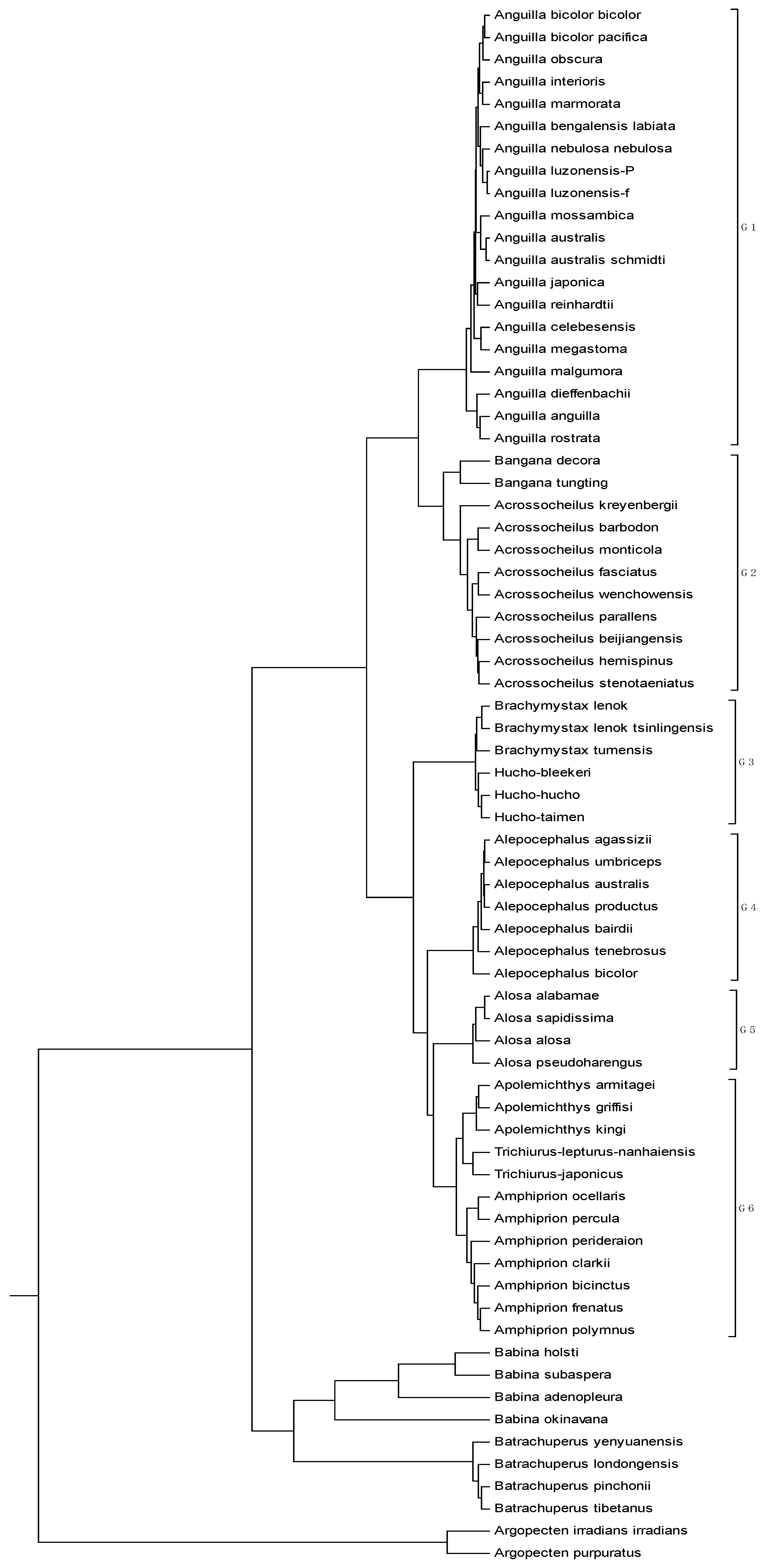
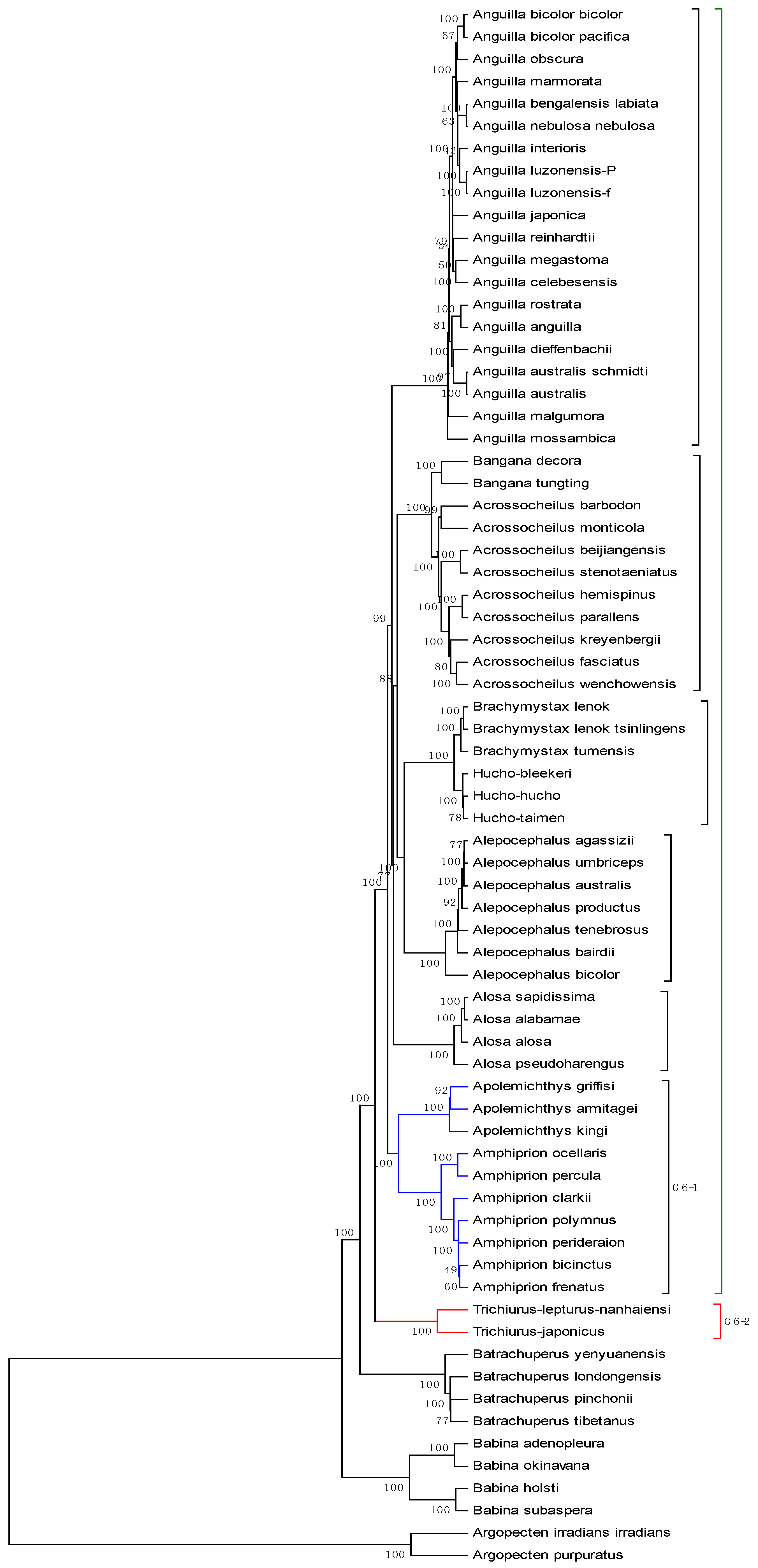
The mitogenome dataset comprises 70 complete mitochondrial genomes of Eukaryota. The name, accession number, and genome length are listed in Table 6. Among them, two species (Argopecten irradians irradians and Argopecten purpuratus) belong to family Pectinidae are used as the out-group. Four species belong to the Order Caudata under the Class Amphibia, while four species belong to the Order Anura under the same Class. The remaining belongs to the Class Actinopterygii. The average length of the 70 genome sequences is about 16817 bp. Thus, K is calculated as 6, and each of these genome sequences is converted into an 18-D vector. The phylogenetic tree constructed by our method is shown in Figure 6. It is easy to see from Figure 6 that the two Pectinidae species stay outside of the others, while the four Hynobiidae species and four Ranidae species form an independent branch. In the subtree of the Class Actinopterygii, the 60 genomes are separated into six groups: group 1 corresponds to genus Anguilla under family Anguillidae; group 2 includes genera Bangana and Acrossocheilus under family Cyprinidae; group 3 includes genera Brachymystax and Hucho under family Salmonidae; group 4 is genus Alepocephalus under family Alepocephalidae; group 5 is the family of Clupeidae; group 6 includes genera Trichiurus, Amphiprion and Apolemichthys under Acanthomorphata. This result agrees well with the established taxonomic groups. In addition, we make a comparison for the 70 genome sequences by using ClustalX2.1 [38], and the corresponding tree is shown in Figure 7. Observing Figure 7, we find that the tree includes four branches: the outside is the Argopecten branch, the following is Babina, then Batrachuperus, and the subtree consisting of the other 60 species. A closer look at the subtree shows that Trichiurus is distinguished from the remaining, which seems to be a disappointing phenomenon in the evolutionary sense.

4. Concluding Remarks

By means of a regular tetrahedron whose center is at the origin, we associate the ten 2-combinations of multiset { · A , · G , · C , · T } with ten unit vectors (points on a unit sphere), and then a novel 3-D graphical representation of a DNA sequence is proposed. Moreover, we partition the graph into K cells, and then a 3K-dimensional cell-based vector is used to numerically characterize a DNA sequence. The proposed method is tested by phylogenetic analysis on four datasets. In comparison with other methods, our approach does not depend on multiple sequence alignment, and avoids the complex calculation as in the calculation of invariants for higher order matrices. Nevertheless, K, the number of cells, is dataset specific, which may restrict our approach. We will make efforts in our future work to find a possible formula for K that is independent of the dataset.

Acknowledgments

The authors wish to thank the three anonymous referees for their valuable suggestions and support. This work was partially supported by the National Natural Science Foundation of China (No. 11171042), the Program for Liaoning Innovative Research Team in University (LT2014024), the Liaoning BaiQianWan Talents Program (2012921060), and the Open Project Program of Food Safety Key Lab of Liaoning Province (LNSAKF2011034).

Author Contributions

Chun Li and Xiaoqing Yu conceived the study and drafted the manuscript. Wenchao Fei and Yan Zhao participated in the design of the study and analysis of the results.

Conflicts of Interest

The authors declare no conflict of interest.

References

  1. Tian, K.; Yang, X.Q.; Kong, Q.; Yin, C.C.; He, R.L.; Yau, S.S.T. Two dimensional Yau-hausdorff distance with applications on comparison of DNA and protein sequences. PLoS ONE 2015, 10. [Google Scholar] [CrossRef] [PubMed]
  2. Hamori, E.; Ruskin, J. H curves, a novel method of representation of nucleotide series especially suited for long DNA sequences. J. Biol. Chem. 1983, 258, 1318–1327. [Google Scholar] [PubMed]
  3. Gates, M.A. Simpler DNA sequence representations. Nature 1985, 316. [Google Scholar] [CrossRef]
  4. Nandy, A. A new graphical representation and analysis of DNA sequence structure: I methodology and application to globin genes. Curr. Sci. 1994, 66, 309–314. [Google Scholar]
  5. Nandy, A. Graphical representation of long DNA sequences. Curr. Sci. 1994, 66, 821. [Google Scholar]
  6. Leong, P.M.; Morgenthaler, S. Random walk and gap plots of DNA sequences. Comput. Appl. Biosci. 1995, 11, 503–507. [Google Scholar] [CrossRef] [PubMed]
  7. Jeffrey, H.J. Chaos game representation of gene structure. Nucleic Acids Res. 1990, 18, 2163–2170. [Google Scholar] [CrossRef] [PubMed]
  8. Randic, M.; Vracko, M.; Nandy, A.; Basak, S.C. On 3-D graphical representation of DNA primary sequences and their numerical characterization. J. Chem. Inf. Comput. Sci. 2000, 40, 1235–1244. [Google Scholar] [CrossRef] [PubMed]
  9. Randic, M.; Novic, M.; Plavsic, D. Milestones in graphical bioinformatics. Int. J. Quantum Chem. 2013, 113, 2413–2446. [Google Scholar] [CrossRef]
  10. Randic, M.; Zupan, J.; Balaban, A.T.; Vikic-Topic, D.; Plavsic, D. Graphical representation of proteins. Chem. Rev. 2011, 111, 790–862. [Google Scholar] [CrossRef] [PubMed]
  11. Li, C.; Tang, N.N.; Wang, J. Directed graphs of DNA sequences and their numerical characterization. J. Theor. Biol. 2006, 241, 173–177. [Google Scholar] [CrossRef] [PubMed]
  12. Yang, Y.; Zhang, Y.Y.; Jia, M.D.; Li, C.; Meng, L.Y. Non-degenerate graphical representation of DNA sequences and its applications to phylogenetic analysis. Comb. Chem. High Throughput Screen. 2013, 16, 585–589. [Google Scholar] [CrossRef] [PubMed]
  13. Gonzzlez-Diaz, H.; Perez-Montoto, L.G.; Duardo-Sanchez, A.; Paniagua, E.; Vazquez-Prieto, S.; Vilas, R.; Dea-Ayuela, M.A.; Bolas-Fernandez, F.; Munteanu, C.R.; Dorado, J.; et al. Generalized lattice graphs for 2D-visualization of biological information. J. Theor. Biol. 2009, 261, 136–147. [Google Scholar] [CrossRef] [PubMed]
  14. Zhang, Z.J. DV-Curve: A novel intuitive tool for visualizing and analyzing DNA sequences. Bioinformatics 2009, 25, 1112–1117. [Google Scholar] [CrossRef] [PubMed]
  15. Qi, Z.H.; Jin, M.Z.; Li, S.L.; Feng, J. A protein mapping method based on physicochemical properties and dimension reduction. Comput. Biol. Med. 2015, 57, 1–7. [Google Scholar] [CrossRef] [PubMed]
  16. Waz, P.; Bielinska-Waz, D. 3D-dynamic representation of DNA sequences. J. Mol. Model. 2014, 20. [Google Scholar] [CrossRef] [PubMed]
  17. Yao, Y.H.; Yan, S.; Han, J.; Dai, Q.; He, P.A. A novel descriptor of protein sequences and its application. J. Theor. Biol. 2014, 347, 109–117. [Google Scholar] [CrossRef] [PubMed]
  18. Ma, T.T.; Liu, Y.X.; Dai, Q.; Yao, Y.H.; He, P.A. A graphical representation of protein based on a novel iterated function system. Phys. A 2014, 403, 21–28. [Google Scholar] [CrossRef]
  19. Zhang, R.; Zhang, C.T. A brief review: The Z curve theory and its application in genome analysis. Curr. Genom. 2014, 15, 78–94. [Google Scholar] [CrossRef] [PubMed]
  20. Zhang, C.T.; Zhang, R.; Ou, H.Y. The Z curve database: A graphic representation of genome sequences. Bioinformatics 2003, 19, 593–599. [Google Scholar] [CrossRef] [PubMed]
  21. Zhang, R.; Zhang, C.T. Z curves, an intuitive tool for visualizing and analyzing DNA sequences. J. Biomol. Struct. Dyn. 1994, 11, 767–782. [Google Scholar] [CrossRef] [PubMed]
  22. Herisson, J.; Payen, G.; Gherbi, R. A 3D pattern matching algorithm for DNA sequences. Bioinformatics 2007, 23, 680–686. [Google Scholar] [CrossRef] [PubMed]
  23. Bianciardi, G.; Borruso, L. Nonlinear analysis of tRNAs squences by random walks: Randomness and order in the primitive information polymers. J. Mol. Evol. 2015, 80, 81–85. [Google Scholar] [CrossRef] [PubMed]
  24. Ghosh, A.; Nandy, A. Graphical representation and mathematical characterization of protein sequences and applications to viral proteins. Adv. Protein Chem. Struct. Biol. 2011, 83. [Google Scholar] [CrossRef]
  25. Karlin, S.; Burge, C. Dinucleotide relative abundance extremes: A genomic signature. Trends Genet. 1995, 11, 283–290. [Google Scholar] [PubMed]
  26. Karlin, S. Global dinucleotide signatures and analysis of genomic heterogeneity. Curr. Opin. Microbiol. 1998, 1, 598–610. [Google Scholar] [CrossRef]
  27. Yang, X.W.; Wang, T.M. Linear regression model of short k-word: A similarity distance suitable for biological sequences with various lengths. J. Theor. Biol. 2013, 337, 61–70. [Google Scholar] [CrossRef] [PubMed]
  28. Li, C.; Ma, H.; Zhou, Y.; Wang, X.; Zheng, X. Similarity analysis of DNA sequences based on the weighted pseudo-entropy. J. Comput. Chem. 2011, 32, 675–680. [Google Scholar] [CrossRef] [PubMed]
  29. Rocha, E.P.; Viari, A.; Danchin, A. Oligonucleotide bias in Bacillus subtilis: General trends and taxonomic comparisons. Nucleic Acids Res. 1998, 26, 2971–2980. [Google Scholar] [CrossRef] [PubMed]
  30. Pride, D.T.; Meineramann, R.J.; Wassenaar, T.M.; Blaser, M.J. Evolutionary implications of microbial genome tetranucleotide frequency biases. Genome Res. 2003, 13, 145–158. [Google Scholar] [CrossRef] [PubMed]
  31. Li, C.; Wang, J. Numerical characterization and similarity analysis of DNA sequences based on 2-D graphical representation of the characteristic sequences. Comb. Chem. High. Throughput Screen. 2003, 6, 795–799. [Google Scholar] [CrossRef] [PubMed]
  32. Li, C.; Wang, J. New invariant of DNA sequences. J. Chem. Inf. Model. 2005, 36, 115–120. [Google Scholar] [CrossRef] [PubMed]
  33. Bai, F.; Zhang, J.; Zheng, J.; Li, C.; Liu, L. Vector representation and its application of DNA sequences based on nucleotide triplet codons. J. Mol. Graph. Model. 2015, 62, 150–156. [Google Scholar] [CrossRef] [PubMed]
  34. MEGA, Molecular Evolutionary Genetics Analysis. Available online: http://www.megasoftware.net (accessed on 15 January 2014).
  35. Wang, J.; Shang, S.Q.; Zhang, Y.L. Phylogenetic relationship of genus catopsilia (Lepidoptera: Pieridae) based on partial sequences of NDI and COI genes from China. Acta. Zootaxon. Sin. 2010, 35, 776–781. [Google Scholar]
  36. Zhang, Y.Z.; Dong, X.; Li, X.; Ma, C.; Xiong, H.P.; Yan, G.J.; Gao, N.; Jiang, D.M.; Li, M.H.; Li, L.P.; et al. Seoul virus and hantavirus disease, Shenyang, People’s Republic of China. Emerg. Infect. Dis. 2009, 15, 200–206. [Google Scholar] [CrossRef] [PubMed]
  37. Yao, P.P.; Zhu, H.P.; Deng, X.Z.; Xu, F.; Xie, R.H.; Yao, C.H.; Weng, J.Q.; Zhang, Y.; Yang, Z.Q.; Zhu, Z.Y. Molecular evolution analysis of hantaviruses in Zhejiang province. Chin. J. Virol. 2010, 26, 465–470. [Google Scholar]
  38. Clustal: Multiple Sequence Alignment. Available online: http://www.clustal.org (accessed on 31 August 2012).
Figure 1. 3-D graphical representation of the sequence ATGGTGCACCTGACTCCTGATCTGGTA.
Applsci 06 00063 g001
Figure 2. (a) The projection on the xy-plane of 3-D curves of 18 DNA sequences; (b) The projection on the yz-plane of 3-D curves of 18 DNA sequences; (c) The projection on the xz-plane of 3-D curves of 18 DNA sequences.
Applsci 06 00063 g002aApplsci 06 00063 g002b
Figure 3. The relationship tree of 18 species.
Applsci 06 00063 g003
Figure 4. The relationship tree of nine COI (cytochrome oxidase subunit I) gene sequences.
Applsci 06 00063 g004
Figure 5. The relationship tree of 34 viruses.
Applsci 06 00063 g005
Figure 6. The tree of 70 genome sequences constructed with the current method.
Applsci 06 00063 g006
Figure 7. The tree of 70 genome sequences constructed with multiple alignment.
Applsci 06 00063 g007
Table 1. The 2-combinations of multiset { · A , · G , · C , · T } .
BaseAGCT
A{A,A}{A,G}{A,C}{A,T}
G-{G,G}{G,C}{G,T}
C--{C,C}{C,T}
T---{T,T}
Table 2. Cartesian 3-D coordinates for the sequence ATGGTGCACCTGACTCCTGATCTGGTA.
PointDinucleotidexyz
1AT010
2TG01−1
3GG0.57740.4226−1.5774
4GT0.57740.4226−2.5774
5TG0.57740.4226−3.5774
6GC0.5774−0.5774−3.5774
7CA0.5774−0.5774−2.5774
8AC0.5774−0.5774−1.5774
9CC0−1.1547−1
10CT−1−1.1547−1
Table 3. The CDS (Coding DNA Sequence) of β-globin gene of 18 species.
No.SpeciesAC (GenBank)Location
1HumanU01317join(62187..62278, 62409..62631, 63482..63610)
2HomoAF007546join(180..271,402..624,1475..1603)
3GorillaX61109join(4538..4630, 4761..4982, 5833..>5881)
4ChimpanzeeX02345join(4189..4293, 4412..4633, 5484..>5532)
5LemurM15734join(154..245, 376..598, 1467..1595)
6CebusaPellaAY279115join(946..1037, 1168..1390, 2218..2346)
7LagothrixLagotrichaAY279114join(952..1043, 1174..1396, 2227..2355)
8BovineX00376join(278..363, 492..714, 1613..1741)
9GoatM15387join(279..364, 493..715, 1621..1749)
10SheepDQ352470join(238..323, 452..674, 1580..1708)
11MouflonDQ352468join(238..323, 452..674, 1578..1706)
12European hareY00347join(1485..1576, 1703..1925, 2492..2620)
13RabbitV00882join(277..368, 495..717, 1291..1419)
14MouseV00722join(275..367, 484..705, 1334..1462)
15RatX06701join(310..401, 517..739, 1377..>1505)
16OpossumJ03643join(467..558, 672..894, 2360..2488)
17GallusV00409join(465..556, 649..871, 1682..1810)
18Muscovy duckX15739join(291..382, 495..717, 1742..1870)
Table 4. The COI (cytochrome oxidase subunit I) genes of nine butterflies.
NO.SpeciesCodeAC (GenBank)Region
1C.pomona pomona f.pomonaPAGU446662Yexianggu, Yunnan
2C.pomona pomona f.hilariaHIGU446664Yexianggu, Yunnan
3C.pomona pomona f.crocaleCRGU446663Menglun, Yunnan
4C.pomona pomona f.catillaCAGU446666Daluo, Yunnan
5C.pomona pomona f.jugurthaJUGU446665Daluo, Yunnan
6C.scylla scyllaCSGU446667Yinggeling, Hainan
7C.pyranthe pyrantheCPGU446668Daluo, Yunnan
8C.pyranthe chryseisCHGU446669Yinggeling, Hainan
9Appias lyncida-GU446670Bawangling, Hainan
Table 5. Sequence information of S segment of hantavirus.
No.StrainAC (GenBank)TypeRegion
1CGRn53EF990907HTNVGuizhou
2CGRn5310EF990906HTNVGuizhou
3CGRn93MP8EF990905HTNVGuizhou
4CGRn8316EF990903HTNVGuizhou
5CGRn9415EF990902HTNVGuizhou
6CGRn93P8EF990904HTNVGuizhou
7CGHu3612EF990909HTNVGuizhou
8CGHu3614EF990908HTNVGuizhou
9Z10AF184987HTNVShengzhou
10Z5EF103195HTNVShengzhou
11NC167AB027523HTNVAnhui
12CGAa4MP9EF990915HTNVGuizhou
13CGAa4P15EF990914HTNVGuizhou
14CGAa1011EF990913HTNVGuizhou
15CGAa1015EF990912HTNVGuizhou
16H5AB127996HTNVHeilongjiang
1776-118M14626HTNVSouth Korea
18Gou3AF184988SEOVJiande
19ZJ5FJ753400SEOVJiande
2080-39AY273791SEOVSouth Korea
21SR11M34881SEOVJapan
22K24-e7AF288653SEOVXinchang
23K24-v2AF288655SEOVXinchang
24Z37AF187082SEOVWenzhou
25ZT10AY766368SEOVTiantai
26ZT71AY750171SEOVTiantai
27K27L08804PUUVRussia
28P360L11347PUUVRussia
29SotkamoX61035PUUVFinland
30Fusong843-06EF488805PUUVJilin
31Fusong199-05EF488803PUUVJilin
32Fusong900-06EF488806PUUVJilin
3391045-AGKF297911PVIran
34I-58KF297914PVIran
Table 6. Sequence information of 70 complete mitogenomes.
No.GenomeAC (GenBank)Length
1Acrossocheilus barbodonNC_02218416596
2Acrossocheilus beijiangensisNC_02820616600
3Acrossocheilus fasciatusNC_02337816589
4Acrossocheilus hemispinusNC_02218316590
5Acrossocheilus kreyenbergiiNC_02484416849
6Acrossocheilus monticolaNC_02214516599
7Acrossocheilus parallensNC_02697316592
8Acrossocheilus stenotaeniatusNC_02493416594
9Acrossocheilus wenchowensisNC_02014516591
10Alepocephalus agassiziiNC_01356416657
11Alepocephalus australisNC_01356616640
12Alepocephalus bairdiiNC_01356716637
13Alepocephalus bicolorNC_01101216829
14Alepocephalus productusNC_01357016636
15Alepocephalus tenebrosusNC_00459016644
16Alepocephalus umbricepsNC_01357216640
17Alosa alabamaeNC_02827516708
18Alosa alosaNC_00957516698
19Alosa pseudoharengusNC_00957616646
20Alosa sapidissimaNC_01469016697
21Amphiprion bicinctusNC_01670116645
22Amphiprion clarkiaNC_02396716976
23Amphiprion frenatusNC_02484016774
24Amphiprion ocellarisNC_00906516649
25Amphiprion perculaNC_02396616645
26Amphiprion perideraionNC_02484116579
27Amphiprion polymnusNC_02382616804
28Anguilla anguillaNC_00653116683
29Anguilla australisNC_00653216686
30Anguilla australis schmidtiNC_00653316682
31Anguilla bengalensis labiataNC_00654316833
32Anguilla bicolor bicolorNC_00653416700
33Anguilla bicolor pacificaNC_00653516693
34Anguilla celebesensisNC_00653716700
35Anguilla dieffenbachiaNC_00653816687
36Anguilla interiorisNC_00653916713
37Anguilla japonicaNC_00270716685
38Anguilla luzonensis (Philippine eel)NC_01157516635
39Anguilla luzonensis (freshwater eel)NC_01343516632
40Anguilla malgumoraNC_00653616550
41Anguilla marmorataNC_00654016745
42Anguilla megastomaNC_00654116714
43Anguilla mossambicaNC_00654216694
44Anguilla nebulosa nebulosaNC_00654416707
45Anguilla obscuraNC_00654516704
46Anguilla reinhardtiiNC_00654616690
47Anguilla rostrataNC_00654716678
48Apolemichthys armitageiNC_02785716551
49Apolemichthys griffisiNC_02759216528
50Apolemichthys kingiNC_02652016816
51Argopecten irradians irradiansNC_01297716211
52Argopecten purpuratusNC_02794316270
53Babina adenopleuraNC_01877118982
54Babina holstiNC_02287019113
55Babina okinavanaNC_02287219959
56Babina subasperaNC_02287118525
57Bangana decoraNC_02622116607
58Bangana tungtingNC_02706916543
59Batrachuperus londongensisNC_00807716379
60Batrachuperus pinchoniiNC_00808316390
61Batrachuperus tibetanusNC_00808516379
62Batrachuperus yenyuanensisNC_01243016394
63Brachymystax lenokNC_01834116832
64Brachymystax lenok tsinlingensisNC_01834216669
65Brachymystax tumensisNC_02467416836
66Hucho bleekeriNC_01599516997
67Hucho huchoNC_02558916751
68Hucho taimenNC_01642616833
69Trichiurus lepturus nanhaiensisNC_01879117060
70Trichiurus japonicusNC_01171916796

