Harmonic Differential Quadrature Analysis of Soft-Core Sandwich Panels under Locally Distributed Loads

Abstract

Sandwich structures are widely used in practice and thus various engineering theories adopting simplifying assumptions are available. However, most engineering theories of beams, plates and shells cannot recover all stresses accurately through their constitutive equations. Therefore, the soft-core is directly modeled by two-dimensional (2D) elasticity theory without any pre-assumption on the displacement field. The top and bottom faces act like the elastic supports on the top and bottom edges of the core. The differential equations of the 2D core are then solved by the harmonic differential quadrature method (HDQM). To circumvent the difficulties in dealing with the locally distributed load by point discrete methods such as the HDQM, a general and rigorous way is proposed to treat the locally distributed load. Detailed formulations are provided. The static behavior of sandwich panels under different locally distributed loads is investigated. For verification, results are compared with data obtained by ABAQUS with very fine meshes. A high degree of accuracy on both displacement and stress has been observed.

1. Introduction

Sandwich beam and plate structures are widely used in aerospace, shipbuilding, construction and other industries due to their high specific stiffness and strength as well as their excellent energy absorption capability. The low weight penalty is especially of vital importance in the design of flight vehicles. Therefore, sandwich structures have received great attention [1]. In practice, the most widely used sandwich beam and plate structures are the sandwich structure having homogeneous face sheets and homogeneous core [2,3]. The face sheets provide the primary load carrying capability, while the core serves to transfer the load between the face sheets. If the core is soft, its deformation effect on the mechanical behavior of the sandwich panel cannot be neglected. Besides, with the development of modern technologies, other types of sandwich structures, which have homogeneous face sheets and non-homogeneous core [4,5] or non-homogeneous face sheets and homogeneous core, exist [6].

The reliability of the response predictions of sandwich structures is critically dependent on the accurate description and numerical simulations of the different phenomena associated with each of the aspects of material behavior [1]. It is found that most engineering theories of beams, plates and shells cannot recover all stresses (e.g., the transverse shear stress) accurately through their constitutive equations. A posteriori stress recovery technique proposed by Tornabene et al. [6,7] may recover the inaccurate stress components based on the accurate in-plane stress components. For simply supported sandwich panels with homogeneous face sheets and core and under sinusoidal loadings, the extended high-order sandwich panel theory (EHSAPT) [3] can yield very accurate stress distributions. In addition, for non-homogeneous core [8] or other loading and boundary conditions [9], the theory cannot recover all stresses accurately through its constitutive equations.

A large variety of classical and advanced plate and shell theories are assessed by Carrera and Brischetto [10,11] to evaluate the bending response of sandwich plate and shell structures with soft cores. It is found that the error sources in the 2D modeling of sandwich plates and shells mainly come from the length-to-thickness-ratio (LTR) and the face-to-core-stiffness-ratio (FCSR). The FCSR error can only be contrasted by using the layerwise analysis [10]. Therefore, a new model where the soft-core is directly modeled by two-dimensional (2D) elasticity theory without a priori assumption [12] is proposed to ensure the accurate stress prediction. The top and bottom faces act like the elastic supports on the top and bottom edges of the core. This model has been proven to be appropriate for modeling the sandwich panels with a soft core [5,12]. Since the solution domain is regular and thus both the differential quadrature method (DQM) and the harmonic differential quadrature method (HDQM) can be employed to solve the problem efficiently.

The DQM, originated by Bellman and Casti in 1971 [13], has been well developed since it was first introduced by Bert et al. [14] for analyzing mechanical behavior of structural components. A variety of problems have been successfully solved thus far [15,16], including beams and plates under point loads that are regarded as very challenging problems for point discrete methods [16,17,18,19,20,21]. In the present investigation, the HDQM is employed.

The HDQM was proposed by Striz et al. [22]. Instead of polynomials used in the DQM, harmonic functions are used in the HDQM to determine the weighting coefficients. The Vandermonde matrix formed by using harmonic functions can be numerically inverted even when the number of points is greater than 15. This indicates that the HDQM is more stable than the DQM. To raise its computational efficiency, explicit formulas to compute the weighting coefficients directly are independently proposed by Wang et al. [23] and Shu et al. [24]. The structure of the weighting coefficients of the HDQM is also studied [25]. Comparative study shows that the HDQM can yield more accurate higher mode frequencies [26]. The HDQM has successfully analyzed the bending of circular plate [27] and geometrically non-linear behavior of doubly curved shell [28]. Civalek combined the HDQM with the DQM or with the finite difference method (FDM) to study the buckling and dynamic behavior of rectangular plates [29,30]. Recently, the HDQM is used to study the buckling and vibration of a pressurized CNT (carbon nano tube) reinforced functionally graded truncated conical shell under an axial compression [31]. Compared with the DQM, however, the HDQM has not been widely used, since its solution accuracy is slightly lower than the DQM when the number of grid points is small and the same when the number of grid points is large.

Obtaining the static behavior of sandwich panels under locally distributed load including the concentrated load is regarded as a challenging problem for point discrete methods such as the DQM and HDQM. Although the problem can be solved using the differential quadrature element method (DQEM) [15,16], difficulty may be also encountered when the load is distributed in a very small area, since the aspect ratio of the element where the load is applied is very large. Besides, the simplicity and computational efficiency may be lost as comparing to the DQM and HDQM, especially when more locally distributed loads are applied on the sandwich panel. In such a case, more differential quadrature elements are required. Therefore, it is desirable to use the DQM or HDQM in the analysis for simplicity and computational efficiency considerations. A general and rigorous way is proposed to obtain the work equivalent load to circumvent the difficulties in dealing with the locally distributed loads by using the HDQM.

The major objective of the present investigation is to use the HDQM for analyzing the static behavior of sandwich panels under locally distributed load. The soft-core is directly modeled by two-dimensional (2D) elasticity theory without a priori assumption. The numerical results are compared with finite element data for verifications. The effects of locally distributed loads on the displacement and stress distributions of the soft-core sandwich panels are investigated. Some conclusions are drawn based on the results reported herein.

2. Theoretical Model

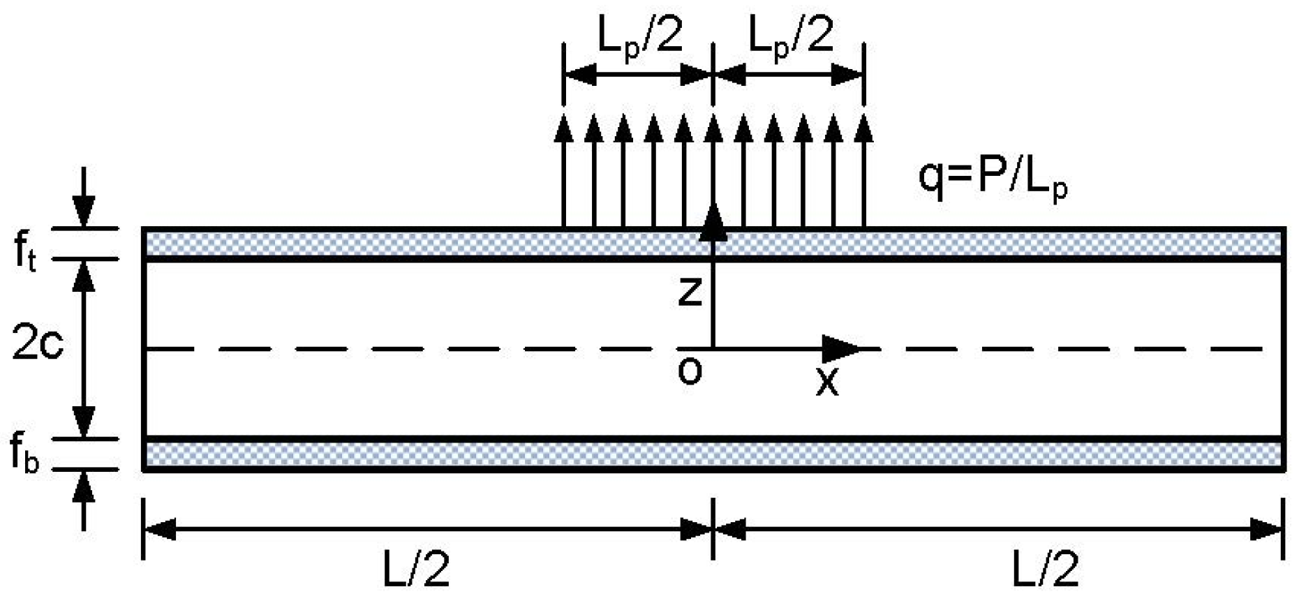
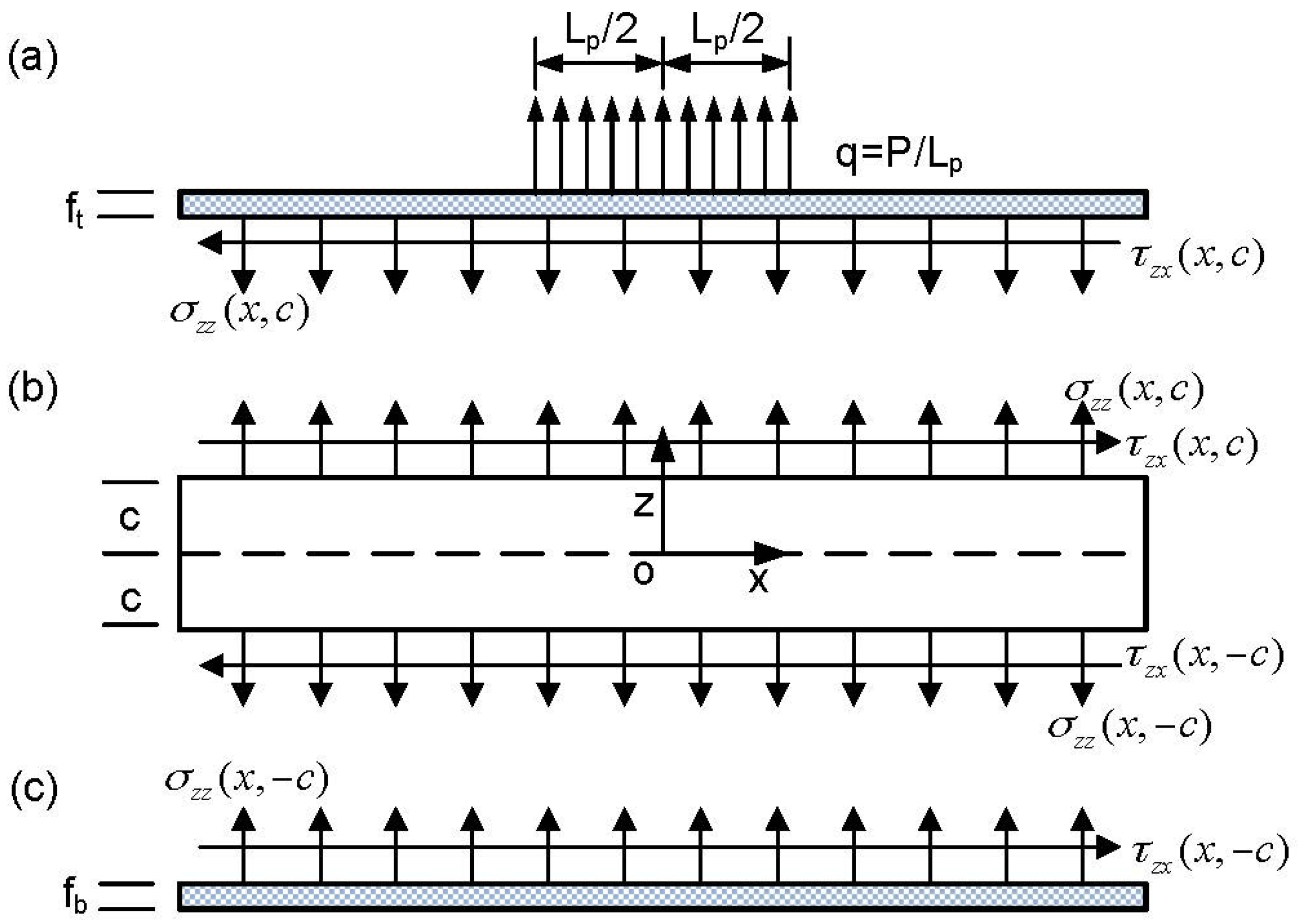
Since most engineering theories of beams, plates and shells cannot recover all stresses accurately through their constitutive equations [6,7], the modeling strategy proposed recently by present authors [12] is employed. A classical sandwich panel shown in Figure 1 is firstly divided into three parts, as shown in Figure 2. The top and bottom face sheets are modeled by Euler–Bernoulli beam theory and the core is directly modeled by two-dimensional (2D) elasticity theory without a priori assumption. After applying the continuity and equilibrium conditions at the interfaces ($z=\pm c$), the resultant differential equations of the top and bottom face sheets are used as the boundary conditions of the 2D core and then only the core needs to be analyzed. In this way, both displacement and stress in the soft-core can be accurately predicted. The Euler–Bernoulli beam assumption is usually adopted in the face sheets of sandwich panel/beam theories, e.g., the extended high-order sandwich panel theory (EHSAPT) [3], which has been validated numerically by present authors [12].

Denote $f_t$, $f_b$ and $2c$ as the thickness of top face, bottom face and the core, respectively. The length of sandwich is L and a unit width is considered.

For simplicity in presentation, the displacement components in x and z directions are denoted by $u(x,z)$ and $w(x,z)$. The material of the core is homogeneous and orthotropic. Therefore, the stress–strain relation is given by

$$\left\{\begin{array}{c}{\mathsf{\sigma }}_{xx}\\ {\mathsf{\sigma }}_{zz}\\ {\mathsf{\tau }}_{xz}\end{array}\right\}=\left[Q\right]\left\{\begin{array}{c}{\mathsf{\epsilon }}_{xx}\\ {\mathsf{\epsilon }}_{zz}\\ {\mathsf{\gamma }}_{xz}\end{array}\right\}=\left[\begin{array}{ccc}{Q}_{11}& Q_{13}& 0\\ Q_{13}& Q_{33}& 0\\ 0& 0& Q_{66}\end{array}\right]\left\{\begin{array}{c}{\mathsf{\epsilon }}_{xx}\\ {\mathsf{\epsilon }}_{zz}\\ {\mathsf{\gamma }}_{xz}\end{array}\right\}=\left[\begin{array}{ccc}\frac{E_{xx}}{1-{\mathsf{\nu }}_{xz}{\mathsf{\nu }}_{zx}}& \frac{{\mathsf{\nu }}_{xz}{E}_{zz}}{1-{\mathsf{\nu }}_{xz}{\nu }_{zx}}& 0\\ \frac{{\mathsf{\nu }}_{zx}{E}_{xx}}{1-{\mathsf{\nu }}_{xz}{\mathsf{\nu }}_{zx}}& \frac{E_{zz}}{1-{\mathsf{\nu }}_{xz}{\mathsf{\nu }}_{zx}}& 0\\ 0& 0& G_{xz}\end{array}\right]\left\{\begin{array}{c}{\mathsf{\epsilon }}_{xx}\\ {\mathsf{\epsilon }}_{zz}\\ {\mathsf{\gamma }}_{xz}\end{array}\right\}$$

(1)

where symbols E, G, and $\mathsf{\nu }$ are elasticity modulus, shear modulus, and Poisson’s ratio, respectively.

The differential equations of the core, shown in Figure 2b, are given by

$$\{\begin{array}{c}{Q}_{11}\frac{{\partial }^{2}u}{\partial x^2}+Q_{66}\frac{{\partial }^{2}u}{\partial z^2}+\left(Q_{13}+Q_{66}\right)\frac{{\partial }^{2}w}{\partial x\partial z}=0\\ Q_{66}\frac{{\partial }^{2}w}{\partial x^2}+Q_{33}\frac{{\partial }^{2}w}{\partial z^2}+\left(Q_{13}+Q_{66}\right)\frac{{\partial }^{2}u}{\partial x\partial z}=0\end{array}$$

(2)

where body forces are not considered.

After applying the continuity and equilibrium conditions at the interface ($z=-c$), the differential equations of the bottom face sheet, shown in Figure 2c, are given by

$$f_b{E}_1^b\left(u_{,xx}^{-c}+0.5f_b{w}_{,xxx}^{-c}\right)+Q_{66}{\left(\frac{\partial w}{\partial x}+\frac{\partial u}{\partial z}\right)}_{z=-c}=0$$

(3)

$$\frac{{f_b}^3}{12}{E}_1^b{w}_{,xxxx}^{-c}-\frac{f_b{Q}_{66}}{2}{\left(\frac{{\partial }^{2}w}{\partial x^2}+\frac{{\partial }^{2}u}{\partial x\partial z}\right)}_{z=-c}-{\left(Q_{13}\frac{\partial u}{\partial x}+Q_{33}\frac{\partial w}{\partial z}\right)}_{z=-c}=0$$

(4)

where $u^{-c}=u(x,-c)$ and $w^{-c}=w(x,-c)$ are displacement components in x and z directions, and $E_1^b$ is the elastic modulus of the bottom face sheet.

Similarly, the differential equations of the top face sheet, shown in Figure 2a, are given by

$$f_t{E}_1^t\left(u_{,xx}^c-0.5f_t{w}_{,xxx}^c\right)-Q_{66}{\left(\frac{\partial w}{\partial x}+\frac{\partial u}{\partial z}\right)}_{z=c}=0$$

(5)

$$\frac{{f_t}^3}{12}{E}_1^t{w}_{,xxxx}^c-\frac{f_t{Q}_{66}}{2}{\left(\frac{{\partial }^{2}w}{\partial x^2}+\frac{{\partial }^{2}u}{\partial x\partial z}\right)}_{z=c}+{\left(Q_{13}\frac{\partial u}{\partial x}+Q_{33}\frac{\partial w}{\partial z}\right)}_{z=c}=q(x)$$

(6)

where $u^c=u(x,c)$ and $w^c=w(x,c)$ are displacement components in x and z directions, $E_1^t$ is the elastic modulus of the top face sheet, and the locally distributed load q(x) is defined as

$$\{\begin{array}{l}q(x)=P/L_p\left(-L_p/2\le x\le L_p/2\right)\\ q(x)=0\hspace{1em}\left(-L/2\le x\le -L_p/2,L_p/2\le x\le L/2\right)\end{array}$$

(7)

In Equation (7), P is the total amount of the applied load on the top face sheet and $L_p$ is the length where the uniform distributed load is applied, shown in Figure 1. In present study, only one locally distributed load applied at the center of the top face is considered. When multiple locally distributed loads are applied at other locations, they can be treated in the same manner as given in the following part.

For the sandwich panel clamped at both ends, denoted by C-C, the boundary conditions are

$$u(\pm L/2,z)=w(\pm L/2,z)=w_{,x}(\pm L/2,\pm c)=0$$

(8)

Note that $w_{,x}(\pm L/2,\pm c)=0$ is due to the Euler–Bernoulli beams fixed at both end and thus should be applied in Equations (3)–(6). Equations (3) and (4) can also be regarded as the elastic (force) boundary conditions applied along edge $z=-c$, and Equations (5) and (6) can be regarded as the elastic (force) boundary conditions applied along edge $z=+c$. For C-C sandwich panel, the force conditions, i.e., Equations (3)–(6), are not applied on the four corner points of the core, since they are fixed and the displacements are zero.

3. Stress Analysis by the HDQM

The system of differential equations is solved numerically by using the HDQM. Hence, the formulations in terms of the harmonic differential quadrature are given in this section. The numbers of grid points in x and z direction are denotes by N and M.

Since the method of modification of weighting coefficient-3 (MMWC-3) [16,32] is used to implement $w_{,x}(\pm L/2,\pm c)=0$ for simplicity, grid V is used in x-direction for reliability consideration. It was observed that the spurious complex eigenvalues of the modified weighting coefficient matrix did not exist if grid V was used [19]. The non-dimensional form of grid V is defined as

$${\mathsf{\xi }}_1=-1,{\mathsf{\xi }}_i=(N-2)\mathrm{Gauss}\mathrm{points}(i=2,3,\mathrm{...},N-1),{\mathsf{\xi }}_N=1$$

(9)

The actual grid coordinates in x-direction are $x_i=L{\mathsf{\xi }}_i/2$, $(i=1,2,\mathrm{...},N)$.

For convenience and accuracy considerations, grid III is used in z-direction. Its non-dimensional form is defined as

$${\mathsf{\eta }}_j=-\cos \left[(j-1)\mathsf{\pi }/(M-1)\right]\hspace{1em}(j=1,2,\mathrm{...},M)$$

(10)

The actual grid coordinates in z-direction are $z_j=c{\mathsf{\eta }}_j$, $(j=1,2,\mathrm{...},M)$.

In terms of harmonic differential quadrature, Equation (2) at all inner grid points are given by

$$\begin{array}{c}\{\begin{array}{l}{Q}_{11}{\displaystyle \sum _{k=2}^{N-1}{B}_{lk}^x{u}_{ik}+Q_{66}{\displaystyle \sum _{j=1}^M{B}_{ij}^z{u}_{jl}}+}\left(Q_{13}+Q_{66}\right){\displaystyle \sum _{j=1}^M}{\displaystyle \sum _{k=2}^{N-1}{A}_{ij}^z{A}_{lk}^x{w}_{jk}}=0\\ Q_{66}{\displaystyle \sum _{k=2}^{N-1}{B}_{lk}^x{w}_{ik}+Q_{33}{\displaystyle \sum _{j=1}^M{B}_{ij}^z{w}_{jl}}+}\left(Q_{13}+Q_{66}\right){\displaystyle \sum _{j=1}^M}{\displaystyle \sum _{k=2}^{N-1}{A}_{ij}^z{A}_{lk}^x{u}_{jk}}=0\end{array}\\ \hfill (i=2,3,\mathrm{...},M-1;l=2,3,\mathrm{...},N-1)\end{array}$$

(11)

where $A_{lk}^x$ and $A_{ij}^z$ are weighting coefficients of the first-order derivative with respect to the variable of x or z, $B_{lk}^x$ and $B_{ij}^z$ are weighting coefficients of the second-order derivative with respect to the variable of x or z, respectively. The fixed boundary conditions, i.e., $u(\pm L/2,z)=w(\pm L/2,z)=$ 0, have been applied.

Explicit formulas to compute the weighting coefficients are available [16,23,24]. $A_{lk}^x$ and $A_{ij}^z$ can be computed by

$$A_{lk}^x=\{\begin{array}{ll}\frac{2p}{L}{\displaystyle \prod _{\begin{array}{l}i=1\\ i\ne l,k\end{array}}^N\sin p({\mathsf{\xi }}_l-{\mathsf{\xi }}_i)}/{\displaystyle \prod _{\begin{array}{l}i=1\\ i\ne k\end{array}}^N\sin p({\mathsf{\xi }}_k-{\mathsf{\xi }}_i)}& (l\ne k)\\ \frac{2p}{L}{\displaystyle \sum _{\begin{array}{l}i=1\\ i\ne l\end{array}}^N\frac{\cos p({\mathsf{\xi }}_l-{\mathsf{\xi }}_i)}{\sin p({\mathsf{\xi }}_l-{\mathsf{\xi }}_i)}}& (l=k)\end{array}$$

(12)

and

$$A_{ij}^z=\{\begin{array}{ll}\frac{p}{c}{\displaystyle \prod _{\begin{array}{l}k=1\\ k\ne i,j\end{array}}^M\sin p({\mathsf{\eta }}_i-{\mathsf{\eta }}_k)}/{\displaystyle \prod _{\begin{array}{l}k=1\\ k\ne l\end{array}}^M\sin p({\mathsf{\eta }}_j-{\mathsf{\eta }}_k)}& (i\ne j)\\ \frac{p}{c}{\displaystyle \sum _{\begin{array}{l}k=1\\ k\ne i\end{array}}^M\frac{\cos p({\mathsf{\eta }}_i-{\mathsf{\eta }}_k)}{\sin p({\mathsf{\eta }}_i-{\mathsf{\eta }}_k)}}& (i=j)\end{array}$$

(13)

where $\mathsf{\xi },\mathsf{\eta }\in [-1,1]$ and p can be 0.5 [23], $\mathsf{\pi }/8$ [16], $\mathsf{\pi }/4$ [24,26,31] or any other values, usually less than 1.0. In present study, p = 0.25. It is not difficult to show that the weighting coefficients are approximately the same as the ones of the DQM when N and M are large enough or p takes a very small number.

$B_{lk}^x$ and $B_{ij}^z$ can be conveniently computed by

$$B_{lk}^x={\displaystyle \sum _{j=1}^N{A}_{lj}^x{A}_{jk}^x},B_{ij}^z={\displaystyle \sum _{k=1}^M{A}_{ik}^z{A}_{kj}^z}$$

(14)

In terms of harmonic differential quadrature, Equations (3) and (4) are expressed by

$$\begin{array}{c}{f}_b{E}_1^b\left({\displaystyle \sum _{k=2}^{N-1}{B}_{lk}^x{u}_{1k}}+0.5f_b{\displaystyle \sum _{k=2}^{N-1}{C}_{lk}^x{w}_{1k}}\right)+Q_{66}\left({\displaystyle \sum _{k=2}^{N-1}{A}_{lk}^x{w}_{1k}+{\displaystyle \sum _{j=1}^M{A}_{1j}^z{u}_{jl}}}\right)=0\hfill \\ \hfill (l=2,3,\mathrm{...},N-1)\end{array}$$

(15)

and

$$\begin{array}{r}\frac{E_1^b{f}_b^3}{12}{\displaystyle \sum _{k=2}^{N-1}{D}_{lk}^x{w}_{1k}-Q_{13}{\displaystyle \sum _{k=2}^{N-1}{A}_{lk}^x{u}_{1k}}-Q_{33}{\displaystyle \sum _{j=1}^M{A}_{1j}^z{w}_{jl}}}\\ -\frac{f_b{Q}_{66}}{2}\left({\displaystyle \sum _{k=2}^{N-1}{B}_{lk}^x{w}_{1k}+{\displaystyle \sum _{j=1}^M}{\displaystyle \sum _{k=2}^{N-1}{A}_{1j}^z{A}_{lk}^x{u}_{jk}}}\right)=0\\ (l=2,3,\mathrm{...},N-1)\end{array}$$

(16)

where

$$C_{lk}^x={\displaystyle \sum _{j=1}^N{A}_{lj}^x{\tilde{B}}_{jk}^x},D_{lk}^x={\displaystyle \sum _{j=1}^N{B}_{lj}^x{\tilde{B}}_{jk}^x}$$

(17)

Note that boundary conditions u_1j = w_1j = 0 (j = 1, N) have been applied. Besides, Equations (15) and (16) are not applied at the two corner points (l = 1, N). In formulating $C_{lk}^x$ and $D_{lk}^x$, $w_{,x}=0$ at nodes 1 and N has been built-in by using MMWC-3 [16,32]. The MMWC-3 is very simple and only ${\tilde{B}}_{jk}^x$ is computed slightly different from Equation (14), namely,

$$\{\begin{array}{l}{\tilde{B}}_{jk}^x={\displaystyle \sum _{l=2}^{N-1}{A}_{jl}^x{A}_{lk}^x}(i=1,N;j=1,2,\mathrm{...},N)\\ {\tilde{B}}_{jk}^x=B_{jk}^x(i=2,3,\mathrm{...},N-1;j=1,2,\mathrm{...},N)\end{array}$$

(18)

Similarly, in terms of harmonic differential quadrature, Equations (5) and (6) are expressed as

$$\begin{array}{r}{f}_t{E}_1^t\left({\displaystyle \sum _{k=2}^{N-1}{B}_{lk}^x{u}_{Mk}}-0.5f_t{\displaystyle \sum _{k=2}^{N-1}{C}_{lk}^x{w}_{Mk}}\right)-Q_{66}\left({\displaystyle \sum _{k=2}^{N-1}{A}_{lk}^x{w}_{Mk}+{\displaystyle \sum _{j=1}^M{A}_{Mj}^z{u}_{jl}}}\right)=0\\ (l=2,3,\mathrm{...},N-1)\end{array}$$

(19)

and

$$\begin{array}{r}\frac{E_1^t{f}_t^3}{12}{\displaystyle \sum _{k=2}^{N-1}{D}_{lk}^x{w}_{Mk}+Q_{13}{\displaystyle \sum _{k=2}^{N-1}{A}_{lk}^x{u}_{Mk}}+Q_{33}{\displaystyle \sum _{j=1}^M{A}_{Mj}^z{w}_{jl}}}\\ -\frac{f_t{Q}_{66}}{2}\left({\displaystyle \sum _{k=2}^{N-1}{B}_{lk}^x{w}_{Mk}+{\displaystyle \sum _{j=1}^M}{\displaystyle \sum _{k=2}^{N-1}{A}_{Mj}^z{A}_{lk}^x{u}_{jk}}}\right)=q_{Ml}\\ (l=2,3,\mathrm{...},N-1)\end{array}$$

(20)

where

$$q_{Ml}=P{\displaystyle \sum _{k=2}^{N-1}{l}_l(L_P{\mathsf{\xi }}_k/2)H_k}/H_{l}L$$

(21)

Note that boundary conditions u_Mj = w_Mj = 0 (j = 1, N) have been applied. Besides, Equations (19) and (20) are not applied at the two corner points (l = 1, N) and Equation (21) is obtained by using the method of work equivalent load. The method is similar to the one proposed by the senior author [16] (pp. 98–99, 125–127) but is more rigorous. Essential to the method is multiplying both sides of Equation (6) by $w^c(x)/2$ and then integrating the resultant equation from −L/2 to L/2 numerically by Gauss quadrature. Differential equations at all integration points are then obtained. Detailed derivations for obtaining the work equivalent load $q_{Ml}$ are included in the Appendix.

Equations (11), (15), (16), (19) and (20) contain 2$(N-2)\times M$ algebraic equations, which can be written in following matrix form,

$$\left[K\right]\left\{U\right\}=\left\{F\right\}$$

(22)

Or in a partitioned form as

$$\left[\begin{array}{cc}\left[k_{uu}\right]& \left[k_{uw}\right]\\ \left[k_{wu}\right]& \left[k_{ww}\right]\end{array}\right]\left\{\begin{array}{c}\left\{u\right\}\\ \left\{w\right\}\end{array}\right\}=\left\{\begin{array}{c}\left\{f_u\right\}\\ \left\{f_w\right\}\end{array}\right\}$$

(23)

where [K] is a non-symmetric full matrix.

Since the fixed boundary conditions have been applied already, displacement vector {U} can be obtained as

$$\left\{U\right\}={\left[K\right]}^{-1}\left\{F\right\}$$

(24)

Once the displacement vector {U} is obtained, the stress components at any grid point of the core can be calculated by

$$\{\begin{array}{c}{\left({\sigma }_{xx}\right)}_{il}=Q_{11}{\displaystyle \sum _{k=2}^{N-1}{A}_{lk}^x{u}_{ik}}+Q_{13}{\displaystyle \sum _{j=1}^M{A}_{ij}^z{w}_{jl}}\\ {\left({\sigma }_{zz}\right)}_{il}=Q_{13}{\displaystyle \sum _{k=2}^{N-1}{A}_{lk}^x{u}_{ik}}+Q_{33}{\displaystyle \sum _{j=1}^M{A}_{ij}^z{w}_{jl}}\\ {\left({\tau }_{xz}\right)}_{il}=Q_{66}\left({\displaystyle \sum _{k=2}^{N-1}{A}_{lk}^x{w}_{ik}+{\displaystyle \sum _{j=1}^M{A}_{ij}^z{u}_{jl}}}\right)\end{array}(i=1,2,\mathrm{...},M,l=1,2,\mathrm{...},N)$$

(25)

4. Results and Discussion

Dimensions of the sandwich panel shown in Figure 1 are f_t = f_b = 2 mm, c = 8 mm and L = 400 mm. The elastic modulus of the graphite/epoxy faces is $E_1^t=E_1^b=$ 181 GPa. The material properties of glass phenolic honeycomb core are $E_{xx}$ = 32 MPa, $E_{zz}$ = 300 MPa, $G_{xz}$ = 48 MPa and v_zx = 0.25. These data are directly taken from [4] for comparison purpose. The normalized deflection $w_n$ is defined as

$$w_n=\frac{3P{L}^3}{2{\mathsf{\pi }}^4{E}_1^t{f}_t^3}$$

(26)

where $P=q{L}_p$ is the total amount of applied load shown in Figure 1. The non-dimensional displacements are the corresponding displacements divided by $w_n$ and the non-dimensional stresses are the corresponding stresses divided by $q=P/L$.

In the literature, the aspect ratio of rectangular plate investigated by using the DQM or HDQM is usually less than 4 and N = M to achieve best accuracy of the solution. For present investigation, the aspect ratio of the core reaches 25, thus N >> M.

To investigate the effect of the number of grid points on the solution accuracy, static analysis of sandwich beams under locally distributed loads is performed by the HDQM with different number (N) of grid points in x direction and M = 9 (fixed). Seven loads are considered, including uniformly distributed load (L_p/L = 1), five locally distributed loads (L_p/L = 0.5, 0.2, 0.1, 0.01, 0.001), and the point load.

Table 1. Convergence study of the HDQ (harmonic differential quadrature) center deflection $w(\pm c,0)/w_n$ for the C-C sandwich panels under locally distributed load (M = 9).

LP		N = 11	N = 21	N = 31	N = 41	N = 51	N = 61	N = 103	ABAQUS
L	c *	0.06780	0.06744	0.06745	0.06745	0.06745	0.06745	0.06745	0.06745
	−c *	0.06770	0.06735	0.06735	0.06735	0.06735	0.06735	0.06735	0.06735
0.5L	c	0.10603	0.10577	0.10576	0.10575	0.10575	0.10575	0.10575	0.10575
	−c	0.10583	0.10556	0.10556	0.10556	0.10556	0.10556	0.10556	0.10556
0.2L	c	0.12740	0.12736	0.12724	0.12725	0.12726	0.12725	0.12725	0.12725
	−c	0.12692	0.12681	0.12676	0.12676	0.12676	0.12676	0.12676	0.12676
0.1L	c	0.13146	0.13266	0.13288	0.13287	0.13285	0.13285	0.13285	0.13285
	−c	0.13090	0.13172	0.13183	0.13183	0.13183	0.13183	0.13183	0.13183
0.01L	c	0.13287	0.13471	0.13537	0.13553	0.13561	0.13564	0.13567	0.13568
	−c	0.13228	0.13356	0.13387	0.13386	0.13387	0.13387	0.13387	0.13387
0.001L	c	0.13288	0.13473	0.13540	0.13556	0.13564	0.13567	0.13571	0.13572
	−c	0.13230	0.13358	0.13389	0.13388	0.13389	0.13389	0.13389	0.13389
Point load	c	0.13288	0.13473	0.13540	0.13556	0.13564	0.13567	0.13571	0.13572
	−c	0.13230	0.13358	0.13389	0.13388	0.13389	0.13389	0.13389	0.13389

*: c represents w(c, 0); −c represents w(−c, 0).

lists the non-dimensional deflections of top (denoted by c) and bottom (denoted by −c) face sheets at x = 0. N varies from 11 to 103 and M = 9. With the self-written FORTRAN code and using a personal computer, the required CPU (central processing unit) time ranges from several seconds to 2.7 mins. It is believed that with better optimized code and a better computer, less CPU time will be taken. Taking M = 9 is based on the fact of that the variation of displacement in z direction is rather small. Larger M is also tried and the results remain unchanged. Finite element data obtained by ABAQUS (Version 6.13-1, Dassault Systenes Simulia Corporation, Providence, RI, USA) with very fine meshes (2000 × 50) are included in the table for comparisons. The entire sandwich panel is modeled by 100,000 rectangular elements named CPS8R (the 8-node bi-quadratic plane stress element with reduced integration). It is seen that the rate of convergence decrease with the decrease of L_p/L. However, the difference between the HDQM data and finite element data is small when N = 61. When N = 103, the results obtained by the HDQM are almost the same as the ones by ABAQUS. It is also observed that no difference between the locally distributed load (L_p/L = 0.001) and the point load. In other words, the two loading cases are equivalent as was reported early in the buckling analysis of rectangular plates [20,21]. From data presented in Table 1, both formulations and developed programs are verified.

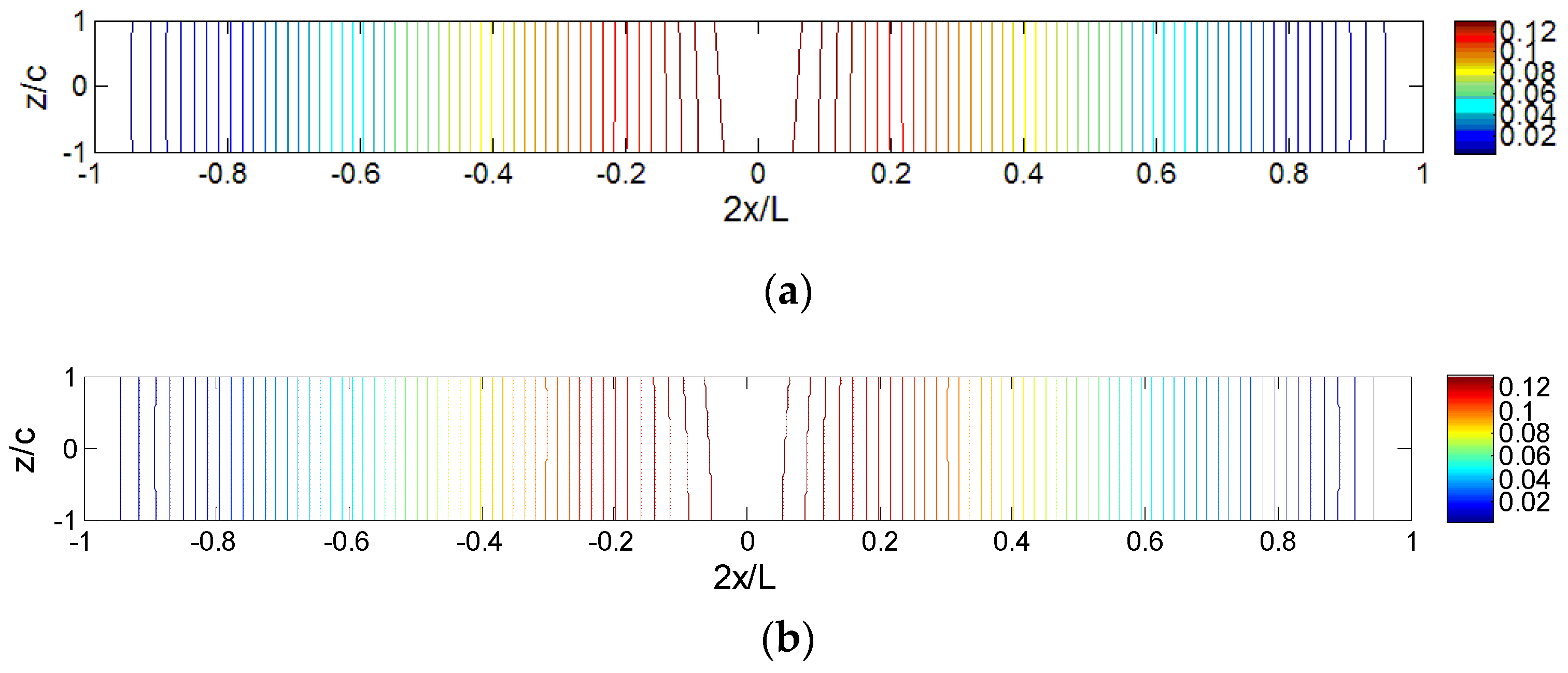
Figure 3 shows the comparison of the core displacement $u/w_n$ obtained by the HDQM and ABAQUS for the C-C sandwich beam under the locally distributed loading (L_p = 0.1L). The data shown in Figure 3 and other figures followed are obtained by using N = 103 to ensure the solution accuracy. Note that the scale in the thickness direction of the plot is enlarged for clarity. In other words, the ratio of unit length in x-direction and z-direction in Figure 3 does not equal to 25. The number of iso-displacement and the color bar may also be slightly different, since they are drawn using different software. It is seen that the HDQ results agree well with the ones of ABAQUS. The through-thickness distribution of the core displacement $u/w_n$ is very complicated due to fixed ends and locally distributed load. It should be pointed out that the magnitude of the axial displacement is very small.

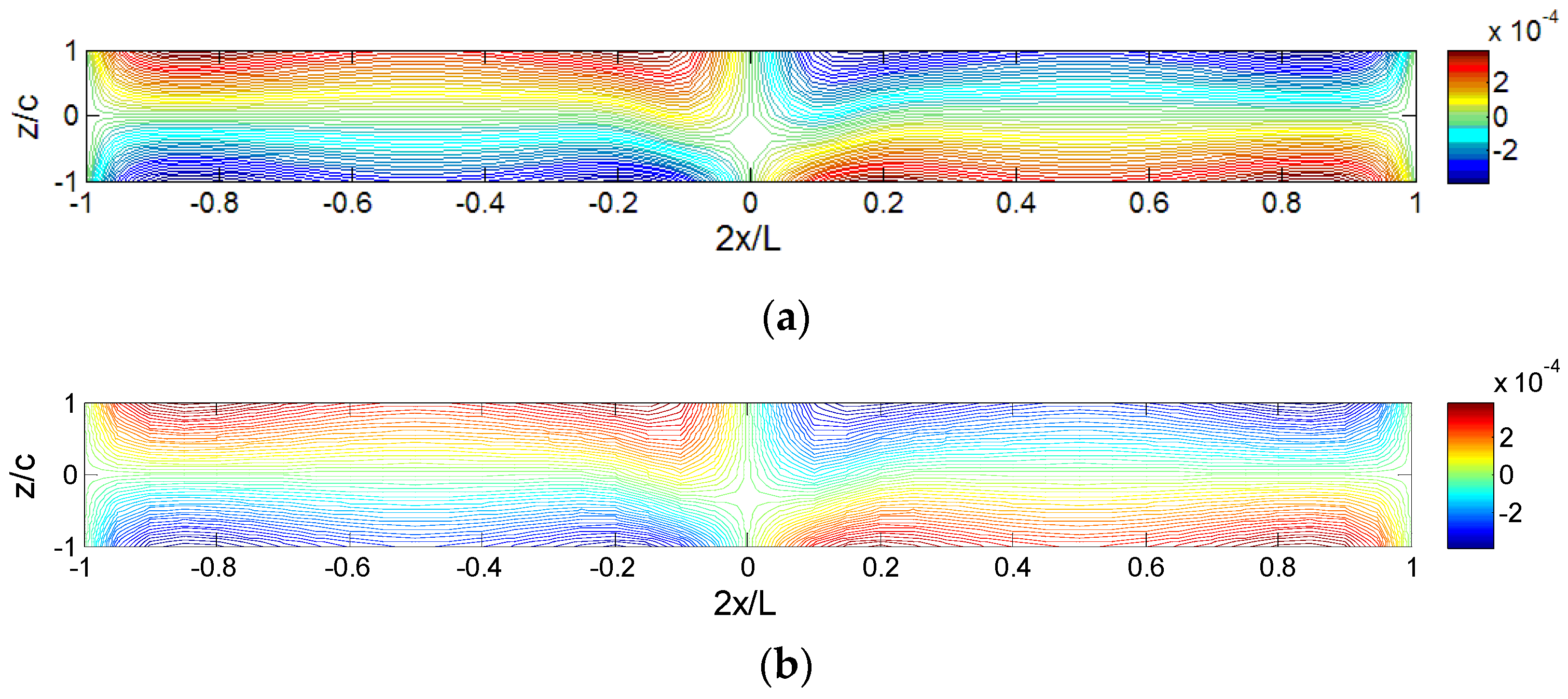
Figure 4 shows the comparison of the core displacement $w/w_n$ obtained by the HDQM and ABAQUS for the C-C sandwich beam under the same loading (L_p = 0.1L). It is seen again that the HDQ results agree well with the ones of ABAQUS. The through-thickness distribution of core displacement $w/w_n$ is very simple and approximately linear in most region of the sandwich panel.

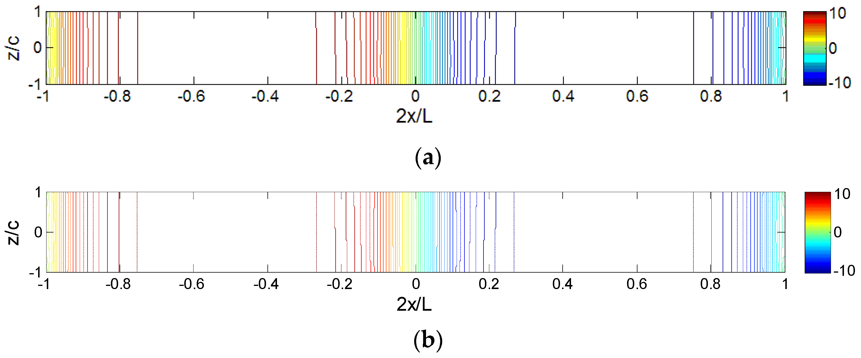
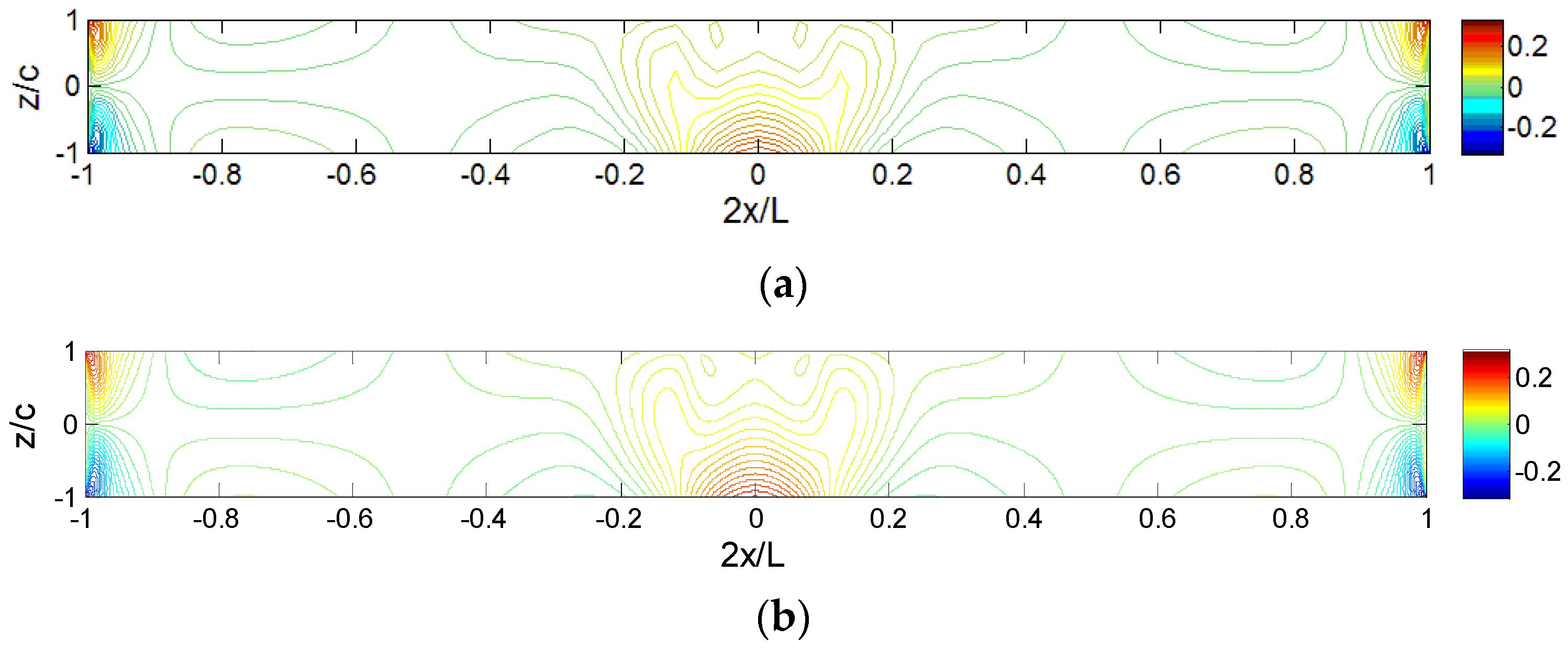
Figure 5 shows the comparisons of iso-stress (${\mathsf{\sigma }}_{xx}/q$) obtained by the HDQM and ABAQUS for the C-C sandwich beam under the locally distributed loading (L_p = 0.1L). Again the scale in the thickness direction is enlarged for clarity. It is seen that the HDQ results agree well with the ones of ABAQUS. The through-thickness distribution of the core stress (${\mathsf{\sigma }}_{xx}/q$) varies along the axial direction due to fixed ends and locally distributed load. High value of stress is observed at the fixed boundary and the sign change of the curvature near the fixed edge areas causes the larger gradient of core axial stress, since the fixed end bending moment quickly reduces to zero at the inflection point close to the fixed end. At the middle of the sandwich panel, lower part of the core has higher axial stress level than the upper part of the core, although the upper part is closer to the loading area.

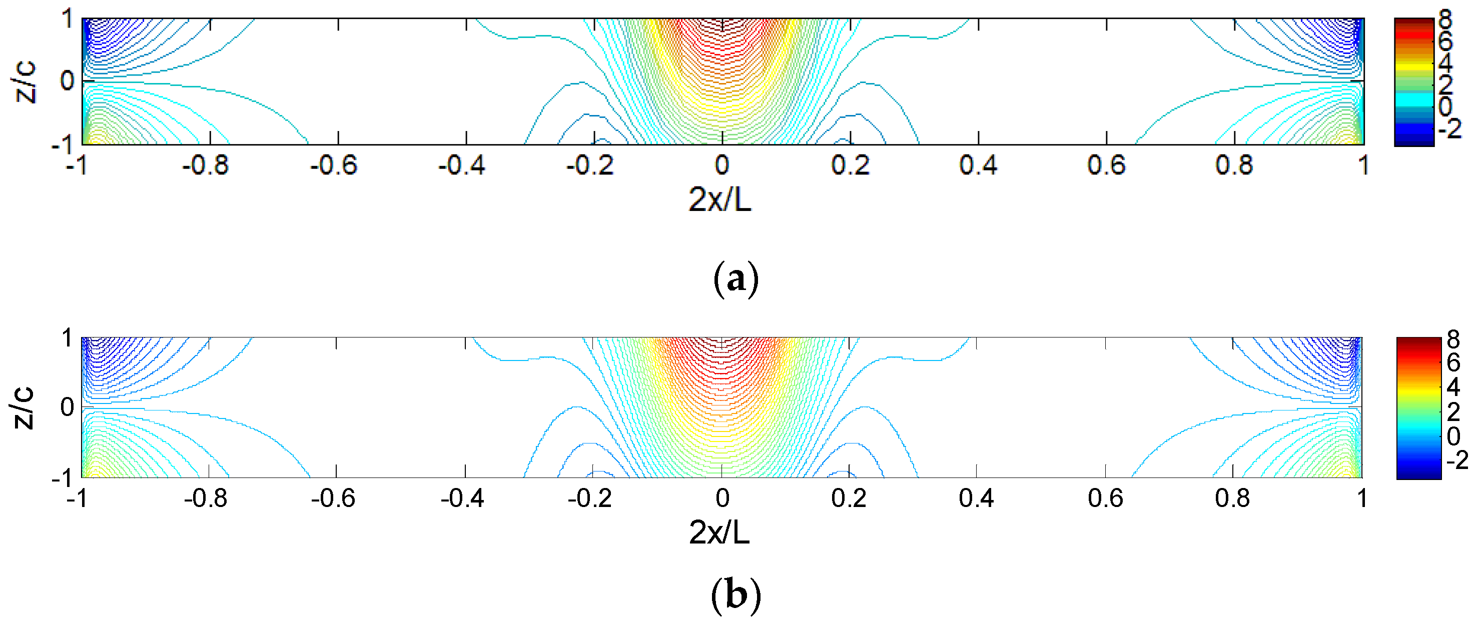
Figure 6 shows the comparisons of iso-stress (${\mathsf{\sigma }}_{zz}/q$) obtained by the HDQM and ABAQUS for the C-C sandwich beam under the same loading (L_p = 0.1L). It is seen that the HDQ results agree well with the ones of ABAQUS. The through-thickness distribution of the core stress (${\mathsf{\sigma }}_{zz}/q$) is also varies along the axial direction due to fixed ends and locally distributed load. The stress at the fixed boundary and loading areas is much higher than other areas. Different from the axial stress distribution, at the middle of the sandwich panel, the upper part of the core sheet, closer to the loading area, has higher transverse stress then the lower part.

Figure 7 shows the comparison of iso-shear-stress (${\mathsf{\tau }}_{xz}/q$) obtained by the HDQM and ABAQUS for the C-C sandwich beam under locally distributed loading (L_p = 0.1L). It is seen that the HDQ results agree well with the ones of ABAQUS. The through-thickness distribution of core shear stress (${\mathsf{\tau }}_{xz}/q$) is simple and close to linear. The larger gradient is observed only at the boundary and loading areas, while the shear stress is almost constant in other areas of the core.

The comparisons of core displacements and stresses, shown in Figure 3, Figure 4, Figure 5, Figure 6 and Figure 7, verify further the correctness of the modeling strategy, the HDQM and the written program.

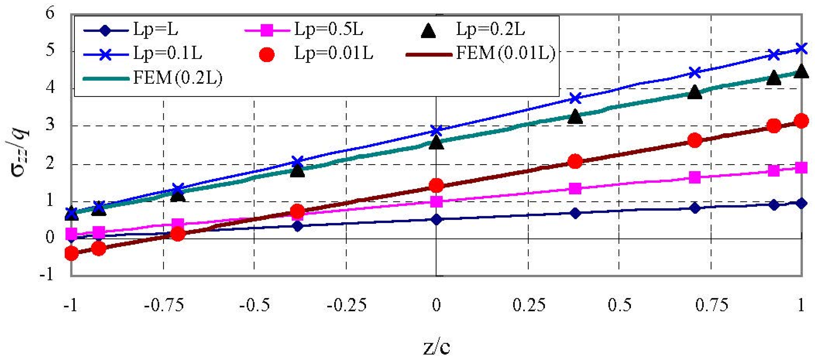
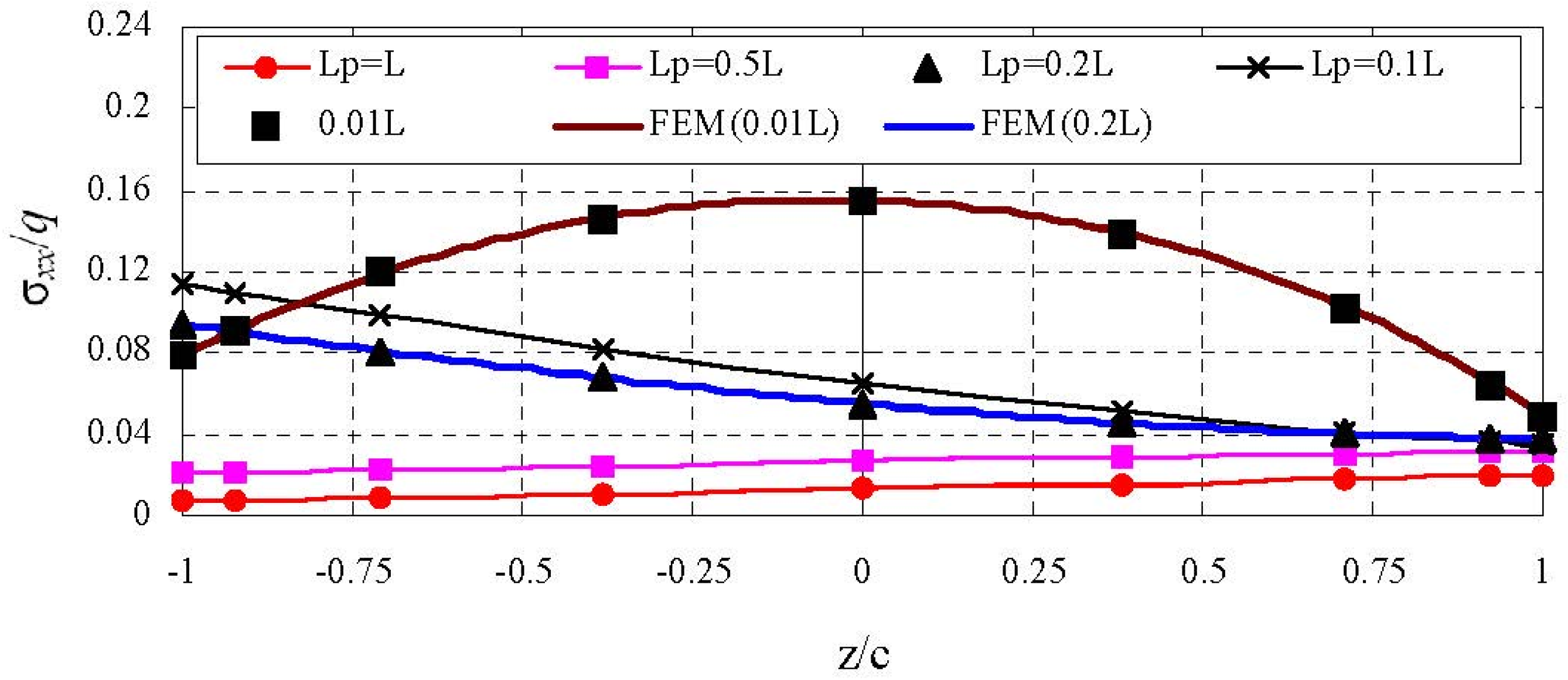
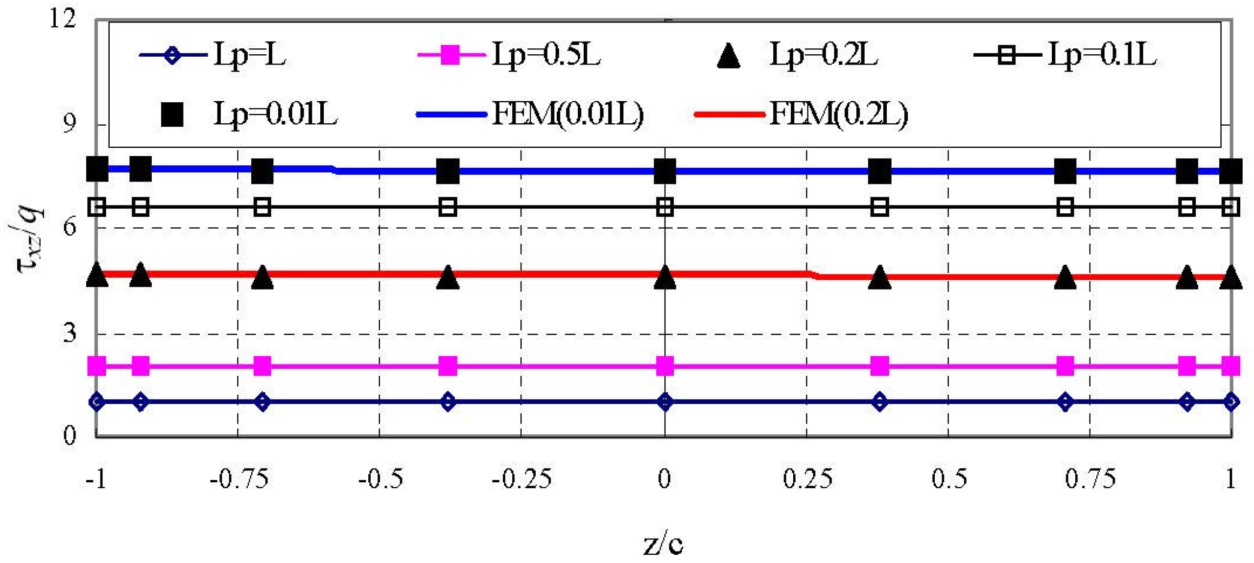
The through-thickness variations of three in-plane stresses with different loading at the section x = −0.0464L are shown in Figure 8, Figure 9 and Figure 10. In the figures, the locally distributed loading for L_p/L = 0.001 and the point load are not included since they almost coincide with the ones of L_p/L = 0.01. Finite element (FE or FEM) data for L_p/L = 0.01 and 0.2 are included for verifications. It is seen that the HDQ data agree well with FE data. For the normalized axial stress ${\mathsf{\sigma }}_{xx}/q$, both the distribution pattern and the location of maximum value depend on the size of the loading area, i.e., the value of L_p/L. The through-thickness variations of ${\mathsf{\sigma }}_{xx}/q$ for loding case of L_p/L = 0.01 is non-linear and approximately linear for all remaining loadings. Both the transverse normal stress and shear stress have similar through-thickness distributions with different size of loading area. The through-thickness variation of ${\mathsf{\sigma }}_{zz}/q$ is approximately linear and the through-thickness variation of ${\mathsf{\tau }}_{xz}/q$ also seems linear but is actually non-linear if smaller scale is used. The maximum of ${\mathsf{\sigma }}_{zz}/q$ is always located at top of the core (z = +c). The Maximum of ${\mathsf{\sigma }}_{xx}/q$ may locate at z = +c when L_p/L is large, i.e., 0.5 and 1.0, or locate at z = −c when loading is limited to a moderate area, i.e., L_p/L = 0.1 and L_p/L = 0.2, or locate at the center of the core when the distributed load is applied at an extremely small area, i.e., L_p/L = 0.01 and 0.001 and even when the point load is applied.

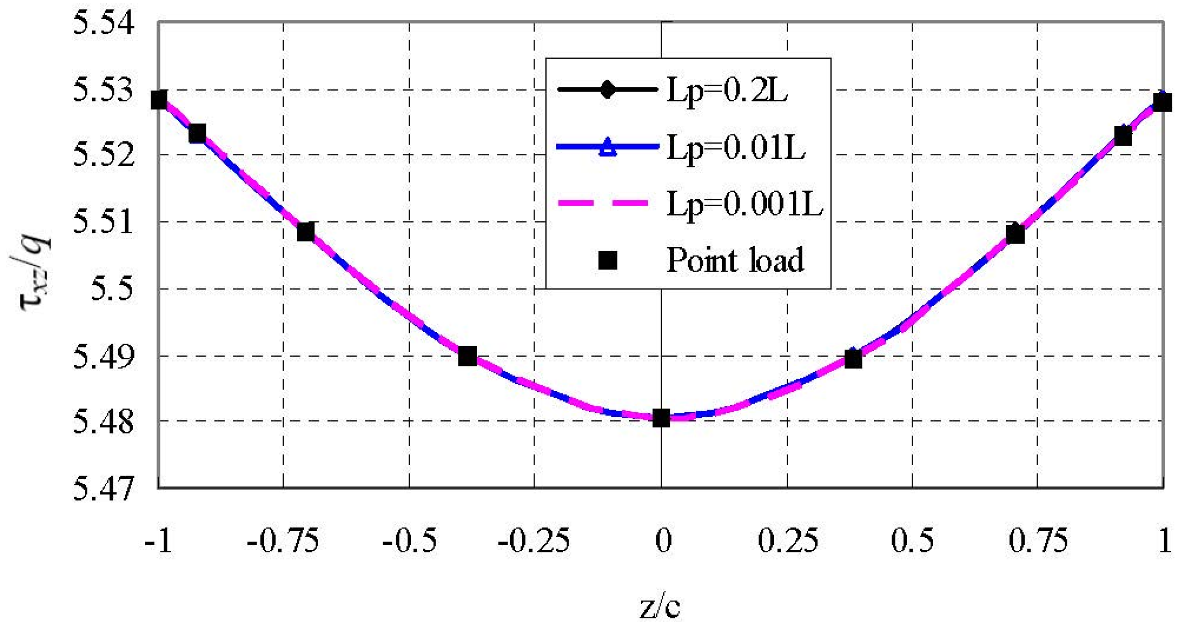
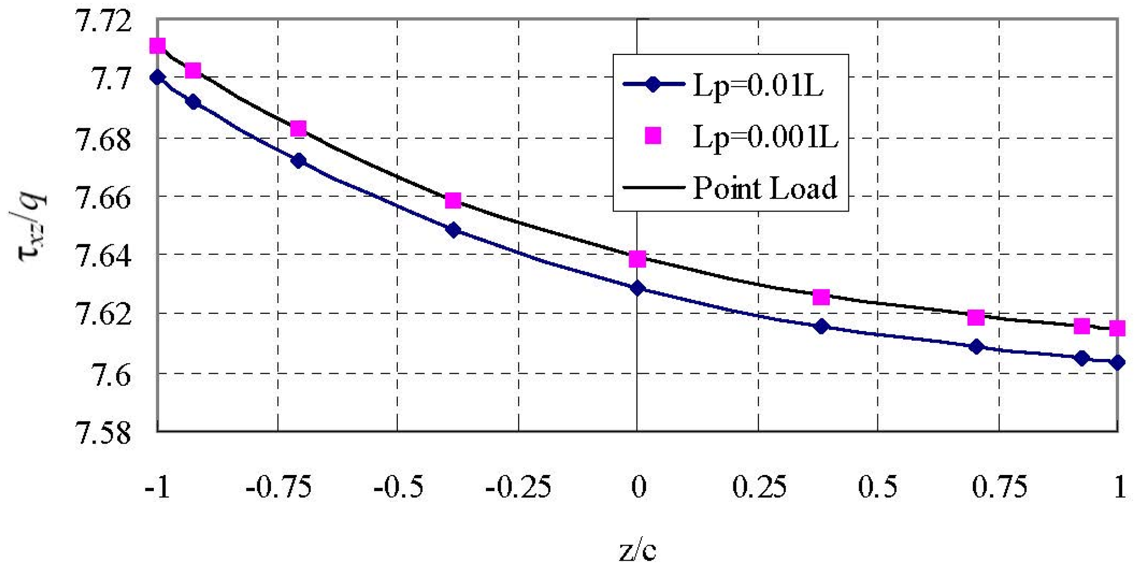
To show the similarity and difference of the through-thickness distributions more clearly for different loadings, much smaller scale than the one in Figure 10 is used in Figure 11 and Figure 12. Figure 11 shows the through-thickness variation of ${\mathsf{\tau }}_{xz}/q$ at section x = −0.0464L which is close to the loading area. Two locally distributed loadins (L_p/L = 0.01 and 0.001) and the point load are considered. It is seen that the through-thickness variation of ${\mathsf{\tau }}_{xz}/q$ is non-linear and small difference between locally distributed load (L_p/L = 0.01) and (L_p/L = 0.001) is observed. However, the small difference cannot be shown on the larger scale in Figure 10. The through-thickness variations of ${\mathsf{\tau }}_{xz}/q$ for the locally distributed load (L_p/L = 0.001) and point load coincide with each other, even in such a small scale. In other words, the two loading cases are identical.

Figure 12 shows the through-thickness variation of ${\mathsf{\tau }}_{xz}/q$ at section x = −0.4726L which is close to the fixed end. Four loading cases are considered. It is seen that the distribution of the shear stress is parabolic and independent on the loadings when $L_P/L\le 0.2$.

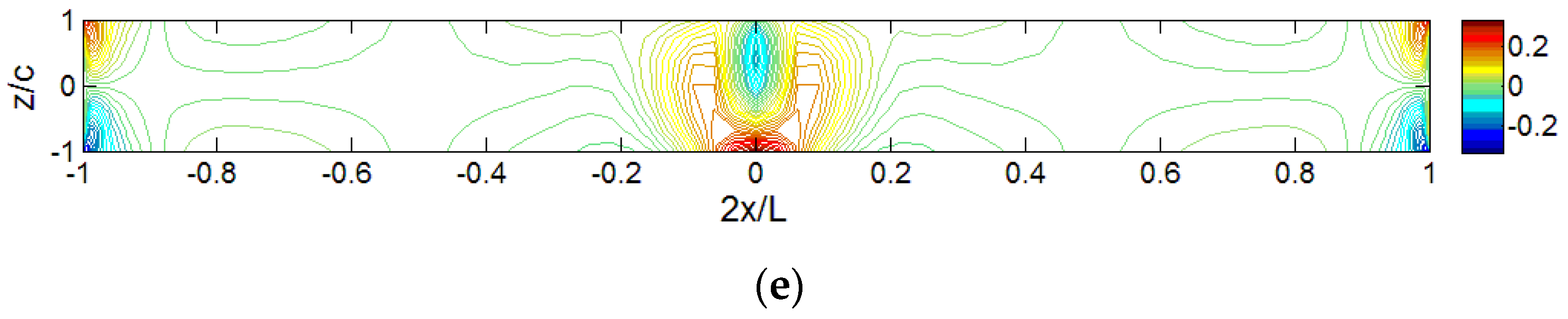
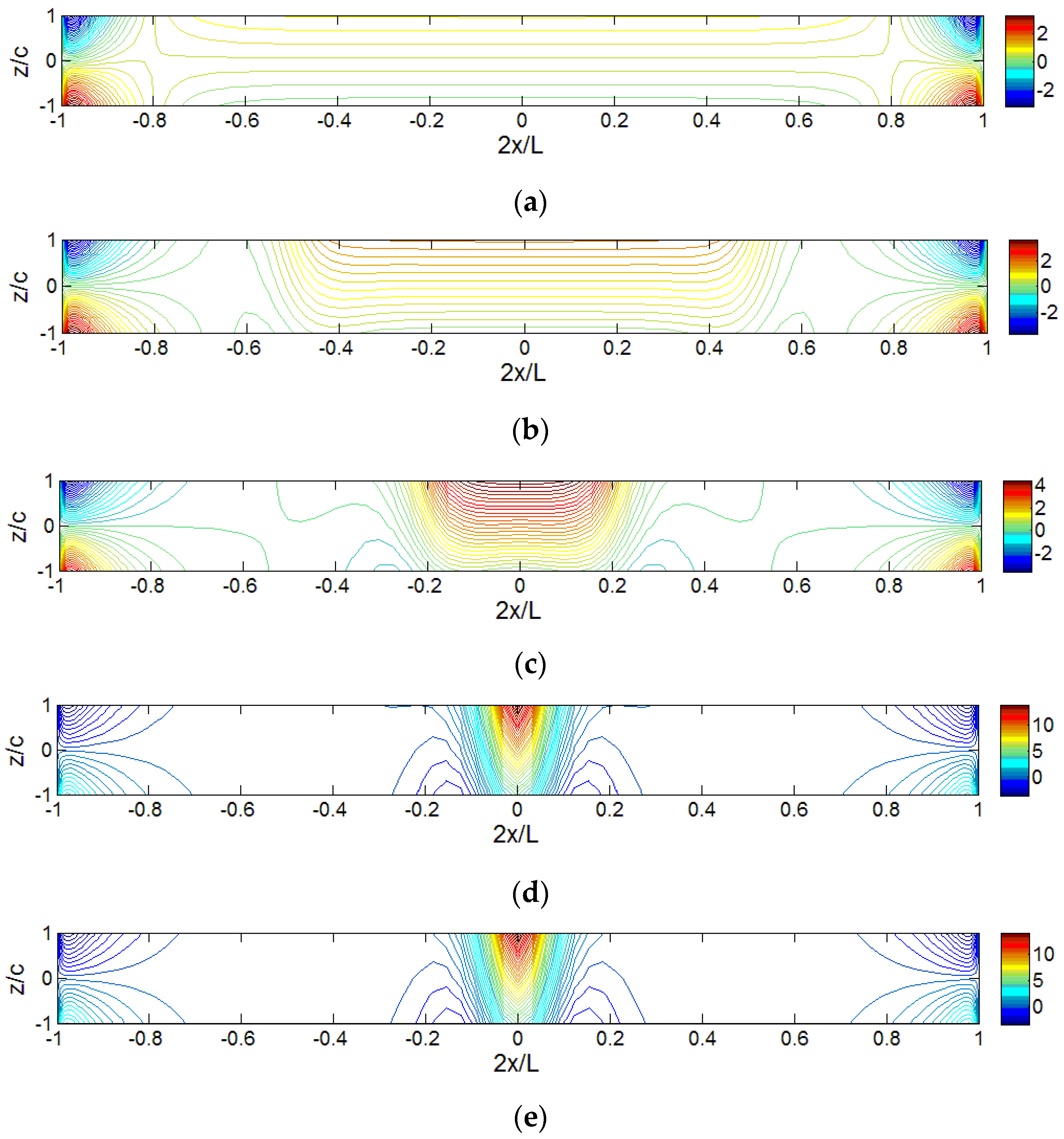
Figure 13 shows the iso-stress (${\mathsf{\sigma }}_{xx}/q$) diagrams for sandwich panels under different distributed loads. Since the diagram for the locally distributed load (L_p/L = 0.1) is already shown in Figure 5 and the diagram for point load is exactly the same as the one for locally distributed load (L_p/L = 0.001), they are not included in Figure 13. The loading effect on the axial stress distributions, especially in the middle area, can be clearly seen. Higher stress appears in the loading area for smaller L_p/L. With extremely small L_p/L, the maximum value located at the lower part of the core, although the upper part is closer to the loading area. For the region away from the loading area ($-0.5L\le x\le -0.3L$ and $0.3L\le x\le 0.5L$), the stress distribution remains similar although L_p/L is quite different.

The iso-stress (${\mathsf{\sigma }}_{zz}/q$) diagrams for sandwich panels under different distributed loads are shown in Figure 14. Since the diagram for the locally distributed load (L_p/L = 0.1) is already shown in Figure 6 and the diagram for point load is exactly the same as the one for locally distributed load (L_p/L = 0.001), they are not included in Figure 14. The loading effect on the transverse normal stress distributions, especially in the middle area, can be clearly seen. Higher stress appears in the loading area for smaller L_p/L. When the load is applied at a wider range, i.e., L_p/L > 0.5, the highest transverse normal stress is observed at the clamped end. Different from the axial stress distribution, the highest magnitude of transverse normal stress changes significant when the size of loading area is changed. In Figure 13a–e, the highest value of ${\mathsf{\sigma }}_{xx}/q$ remains in the same level with different L_p/L cases, while the highest value of ${\mathsf{\sigma }}_{zz}/q$ shown in Figure 14a-e may be increased by several times with smaller L_p/L.

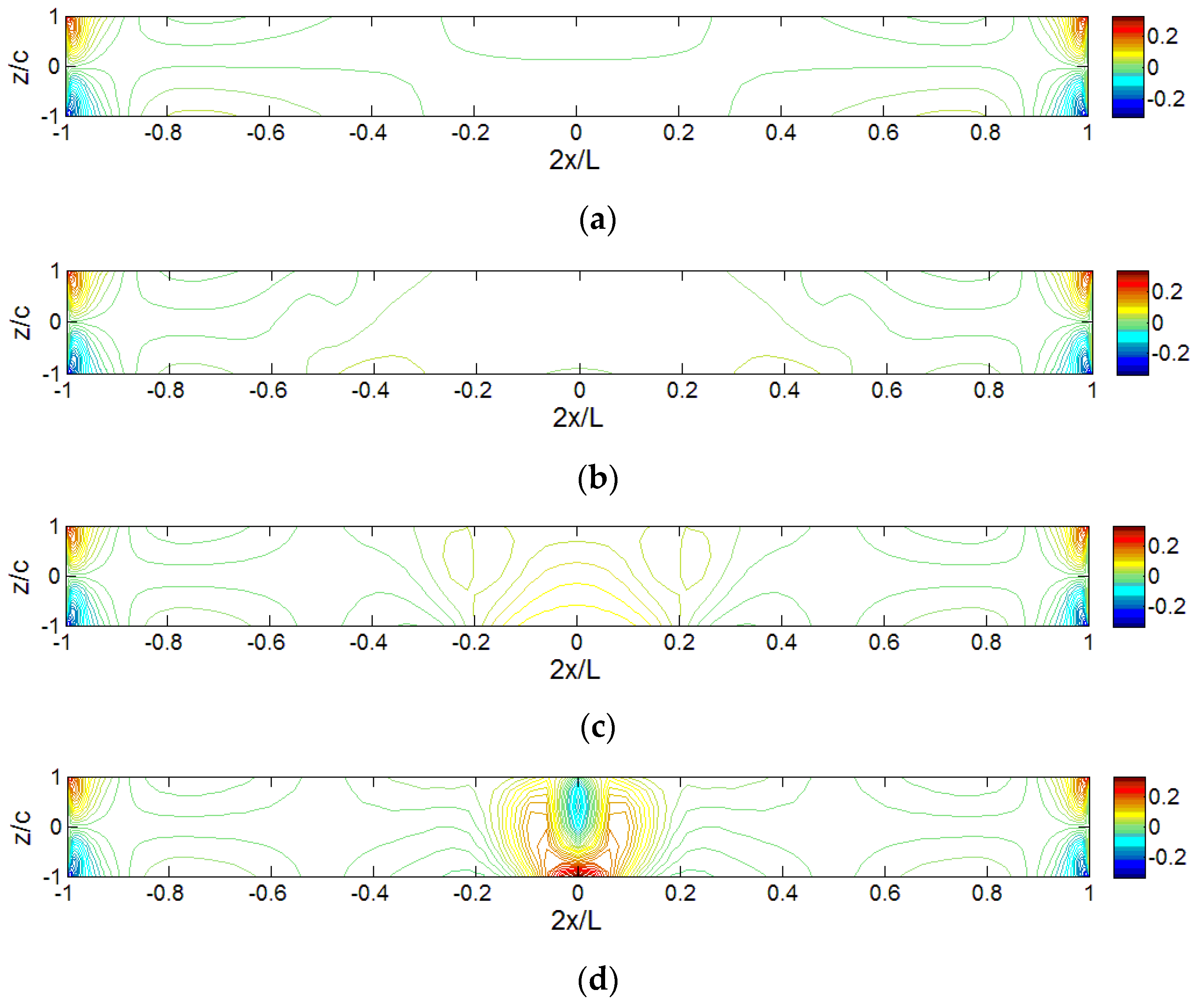
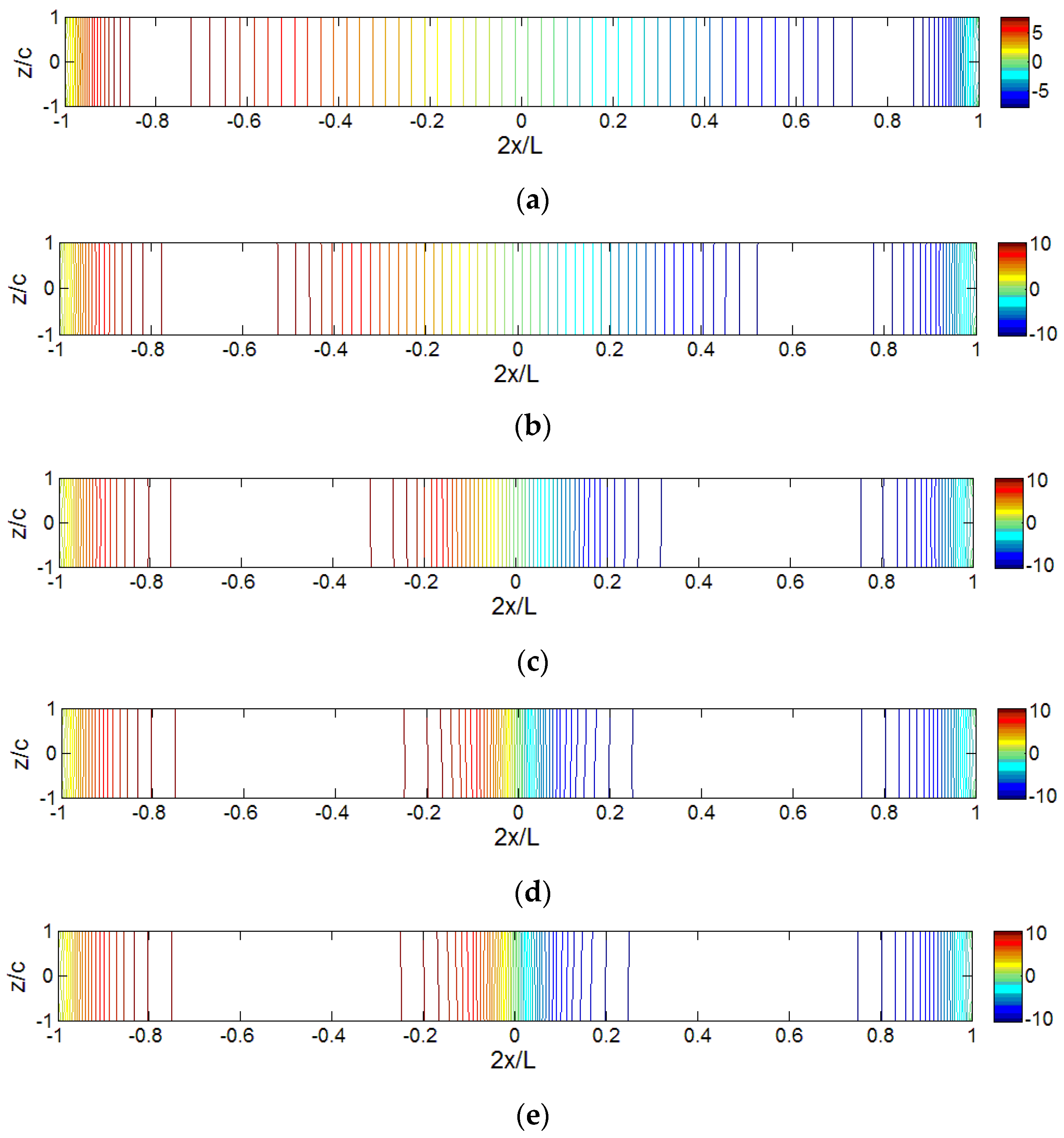
Figure 15 shows the iso-stress (${\mathsf{\tau }}_{xz}/q$) diagrams for sandwich panels under different distributed loads. For the same reason, the diagram for the locally distributed load (L_p/L = 0.1) and the diagram for point load are not included in Figure 15. The loading effect on the transverse shear stress distributions, especially in the middle area, can be clearly seen. It should be pointed out that the through-thickness distribution is actually non-linear, as clearly shown in Figure 11 and Figure 12. Similar to the axial normal stress, the size of loading area, L_p/L, does not affect the maximum value of the normalized shear stress too much.

5. Conclusions

The static behavior of C-C sandwich panels under various locally distributed loads, a challenge problem for point discrete methods, is successfully solved using the HDQM. To circumvent the difficulties in dealing with the locally distributed loads and the point load by the HDQM, the simple and general method of work equivalent load is proposed. The derivations to obtain the work equivalent load are slightly different from the existing one and more rigorous. The recent proposed modeling strategy for the sandwich panels with soft cores are adopted in the analysis. Since the core is modeled directly by 2D elasticity theory without a priori assumption, accurate prediction of the response can be achieved.

Detailed formulations are presented. Seven loadings including the point load are investigated. Convergence studies are performed. Results show that the rate of convergence is high but decreases with decrease of the length where the locally distributed load applies. Due to the large aspect ratio, the number of grid points in x direction is much larger than the one in z direction to achieve the computational efficiency. Comparisons with finite element data obtained by ABAQUS with very fine meshes reveal that numerical results obtained by the HDQM, including displacements and stresses, are highly accurate and can be served as a reference for other investigators during developing their new numerical methods.

Based on the results reported herein, one may conclude that the computational model is found to be appropriate and efficient in analyzing static behavior of sandwich panels with homogeneous orthotropic soft cores. The method of work equivalent load is general and can be used to treat any types of applied loads efficiently. Present investigation extends the application range of the harmonic differential quadrature method.