1. Introduction
Ever since the discovery of androgen dependency of prostate cells, androgen deprivation therapy (ADT) has played a vital role in the treatment of metastatic and locally advanced prostate cancer [
1,
2,
3]. However, controversy remains regarding its best application. Although this treatment will regress tumors in over
of patients [
4], after prolonged androgen depletion, patients will eventually develop castration-resistant prostate cancer (CRPC) [
5]. The development of CRPC can take from a few months to more than ten years [
3,
6], after which there is a very limited number of effective treatments and patients suffer high mortality [
7]. ADT is expensive and its side effects include sexual dysfunction, hot flashes, and fatigue [
8]. Based on some preclinical studies, intermittent androgen suppression (IAS) is suggested as a sensible alternative to ADT [
9]. During off-treatment periods, patients enjoy a “vacation” from the severe side effects of ADT [
8], and studies have suggested that IAS may not negatively affect the time to resistance progression or survival in comparison to ADT [
10]. Consequently, IAS is selected by some patients to improve the quality of life and also hopefully to delay the progression to CRPC [
4].
Many mathematical models have studied the dynamics of prostate cancer during ADT or IAS [
11,
12,
13,
14,
15,
16,
17,
18]. A detailed review of some of these models are presented in the recent book of Kuang et al. [
19]. Ideta et al. are pioneers of mathematically modeling and analyzing the dynamics of IAS [
12]. They formulated a system of ordinary differential equations to study the mechanics of ADT and IAS. They considered castrate-resistant (CR) and castrate-sensitive (CS) cell populations as well as androgen levels. Their model included mutations from CS to CR cells, and their focus was on comparing continuous and intermittent therapy and the development of resistance. Hirata et al. [
14] introduced a piece-wise linear model of three cancer cell populations. Their model included CS cells, CR cells that may mutate into CS cells, and CR cells that will not mutate. Several investigators using Hirata et al.’s model [
14] have studied estimation of parameters [
20,
21], optimal switching times and control in IAS [
20,
22,
23], and forecasting CRPC progression [
24,
25].
Built on the works of Ideta et al. [
12] and Jackson [
26], Portz, Kuang, and Nagy (PKN) [
13] developed a novel mathematical model to study the dynamics of IAS by using the cell quota model [
27] from mathematical ecology, which relates growth rate to an intracellular nutrient, to modeling the growth of both the CS and CR cell populations. The cell quota in [
13] is defined as the intracellular androgen concentrations for each cell population. This model is carefully fitted with clinical prostate-specific antigen (PSA) data, where androgen data was used to model the cell quota and other growth parameters. Everett et al. [
28] compared the models of Hirata et al. [
14] and PKN [
13] regarding their accuracy of fitting clinical data and predicting future PSA levels. They concluded that while a biologically-based model is important to reveal the underlying processes and my present more robust and better predictions, a simpler model such as that of Hirata et al. might also be practical for fitting clinical data and predicting future PSA outcomes of individual patients.
In this paper, we present a simplified model to the final model in PKN [
13]. Several key terms in our model will be mechanistically formulated. This model is concise and amenable to systematical mathematical analysis of its dynamics. For simplicity, we shall use serum androgen concentration to approximate intracellular androgen. This is reasonable since androgen passively and quickly diffuses through the prostate membrane via concentration gradient [
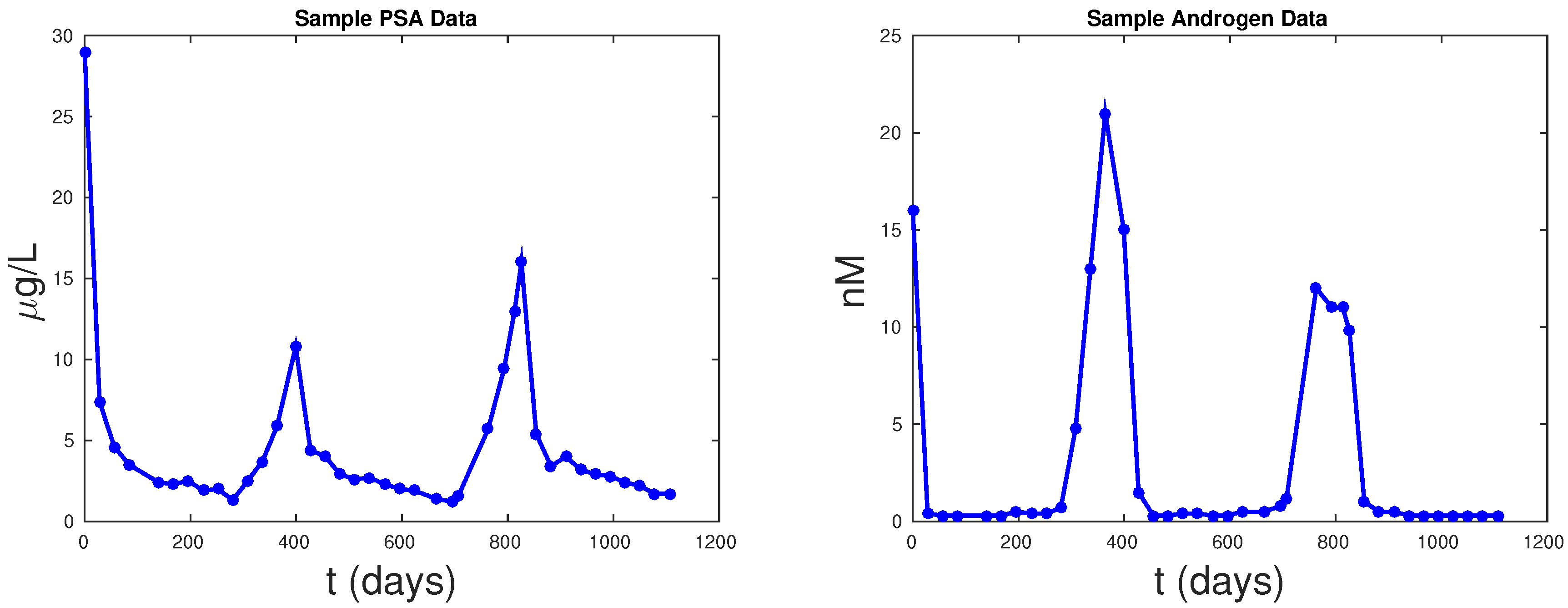
29]. This approach is practical for a typical clinical setting, where the data collected can be applied directly to the model. Most importantly, our model can fit PSA and androgen values simultaneously, which enables us to be more accurate in making future PSA value predictions.
3. Formulation of Mathematical Models
We develop two plausible mathematical models to study the temporal dynamics of prostate cancer progression to CRPR. In Model 1, we do not distinguish CS from CR cells. In this model, tumor cells’ death rate is assumed to be a monotonically decreasing exponential function to implicitly account for the resistance development in cancer cells. Then, we propose a two cell population model where we separate CS from CR cells explicitly. To be more biologically relevant and consistent with the PKN model formulation, we assume in Model 2 that the development of cancer cell resistance to IAS is a decreasing function of androgen levels.
In both models, the cell growth rate is determined by the androgen
. Specifically, as in the PKN model [
13], we model the growth rate by a two parameter function of androgen cell quota,
where
Q is the androgen cell quota. Equation (
1) is known as Droop equation or a Droop growth rate model [
19]. It assumes that
Q is the concentration of the most limiting resource or nutrient, and
q is the minimum level of
Q required to prevent cell death [
27].
To be biologically relevant, for both models, we assume that the initial values for all variables are positive. This shall ensure that all components of their solutions are positive. Accordingly, we are only interested in studying the stabilities of nonnegative steady states and their biological and clinical implications.
3.1. Model 1: Single Population Model
In the following model, tumor cell volume is denoted by
x , and we assume that the total volume is a combination of CS and CR cells. Intracellular androgen cell levels are denoted by
Q (nM), and PSA levels by
P . Droop’s equations govern the growth rate of cancer cells [
27], where
μ represents the maximum cell growth rate and
q the minimum concentration of androgen to sustain the tumor. Similar to [
28], we assume an androgen-dependent death rate, where
R denotes the half saturation level. However, we also assume a time dependent maximum baseline death rate
ν, which decreases exponentially at rate
d to reflect the cell castration-resistance development due to the decreasing death rate. We also include a density-independent death rate
δ that constrains the total volume of cancer cells to be within realistic ranges [
31]:
In this model, androgen is assumed to be the most limiting nutrient. We assume that the androgen concentration in cancer cells is approximately the same as the androgen concentration in serum [
29]. Parameter
denotes the constant production of androgen by the testes, and
denotes the production of androgen by the adrenal gland and kidneys. As over 95% of androgen is produced in the testes, we have that
. Parameter
is a switch between on and off treatment cycles. Luteinizing hormone releasing hormone agonists only stop testes production of androgen during treatment. During treatment,
will be the only production of androgen.
denotes the maximum androgen level in serum. The androgen uptake by prostate cells is assumed to be proportional to the difference of the maximum possible and the current androgen levels in serum. Androgen in cells is depleted for growth at a rate of
. PSA is produced by both the regular cells in the prostate at the rate
and by the cancer cells at the rate
. Notice that we have assumed that cell production of PSA is assumed to be dependent on levels of androgen. Finally, PSA is cleared from serum at rate
ϵ.
3.2. Model 2: Two Population Model
Now, we present a two cell population model. In this model, we explicitly differentiate between CS and CR cells.
and
denote the CS and CR cell populations, respectively. The proliferation of each cancer cell population is denoted by
for
and
respectively. Since CR cell populations proliferate at lower levels of androgen, we assume that
. Death rates are denoted by:
for their respective cell populations. We shall assume that
, as CR cells are less susceptible to apoptosis by androgen deprivation than CS cells. Parameters
denote the density dependent death rates, and we use these parameters to keep the maximum tumor volume in biological ranges.
Mutation between cell populations is assumed to take the form of a Hill equation of coefficient 1, given by:
The CS to CR rate,
, is a decreasing function of the androgen levels. We assume that when cells are experiencing androgen depletion, they have higher selective pressure to develop resistance. Likewise, in an androgen rich environment, CS cells are more likely to stay sensitive. IAS started under this assumption, with the intention to delay resistance [
10].
c is the maximum rate of mutation between cells and
K is the cell concentration for achieving half of the maximum rate of mutation. In this model,
s are held constant and are not time dependent, as the mechanism of the development of resistance is due to mutations from
to
via
and not by a decreasing androgen dependent death rate.
The increase of intracellular androgen levels by diffusion from the serum level is modeled by
. For simplicity, and in contrast to the PKN model [
13] and the model in Morken et al. [
32], we assume the same PSA production rate
σ for both cell populations:
In a biologically realistic situation, one expects that
3.3. Derivation of
Now, we provide a conservation law based derivation for the cell quota
Q Equations (4) and (9). Specifically, we derive Equation (4) in detail and leave to the readers the straightforward task of its extension to (9). Our formulation comes from the conservation of androgen as it moves in and out of the tumor. Let
be the total androgen inside tumor
x . We assume that
Q is uniformly distributed in
x, and
The inflow of androgen to the tumor comes from the serum which can be approximated by
The outflow of androgen from the tumor is due to death, which is
Then, the rate of change of androgen inside the tumor is:
However,
which implies that
A similar approach can be applied to derive for Model 2.
3.4. Portz, Kuang, and Nagy (PKN) Model
In this section, we briefly review the PKN model. For a more detailed explanation of this model, the reader is referred to [
13]. The PKN model assumes constant death rates for cancer cells (
). CS and CR cells have androgen cell quota
respectively.
A denotes the serum androgen concentration, which is interpolated and used in the model:
4. Model Dynamics
Now, we study the mathematical properties and dynamics of our two models. For Model 1, we shall state the results without providing proofs as they are routine. The detailed mathematical analysis for Model 2 will be presented. Proposition 1 summarizes the mathematical dynamics of Model 1. Since
P is decoupled from the system, we shall refer only to the dynamics of Equations (
2)–(4). This proposition reveals that there is no cure for cancer. Since ADT is non-curative, this property is biologically reasonable.
Proposition 1. Solutions of the system Equations (2)–(4) are positive and bounded. The system Equations (2)–(4) has a cancer free steady state that is unstable, and a steady state that is globally stable.
Next, we do a thorough mathematical analysis of Model 2. First, we study boundedness and positivity of the system. Followed by the number and existence of steady states. Finally, we analyze the local stability of the steady states. Observe that P is also decoupled from Equations (2)–(4) and we do not include it in the analysis.
Proposition 2. Assume and Then, solutions of Equations (7)–(9) with initial conditions , , and stay in the region , where .
Proof. We note that in Equation (7), appears in every term ensuring its positivity. Since appears in the first two terms of (8) and appears in the last term, the positivity of is also guaranteed.
In addition,
and
We see that and It is thus easy to see that for with initial conditions .
For boundedness of
and
, we let
. Since we have that
, and the growth rate
are increasing functions of
Q, we have
which implies that
. ☐
Now, we study the steady states of Model 2. We seek to understand the conditions under which one population will overtake the other, and the circumstances under which they may coexist.
Proposition 3. Assume and The system Equations (7)–(9) have a CR cell only steady state , and a coexistence steady state where and .
Proof. Let be a steady state of the system Equations (7)–(9). We have two mutually exclusive cases: and
If , then we have two possibilities: (i) or (ii) . In the case of (i), we see that In the case of (ii), we see that
If
we see that
from the equation of
In this case,
In addition, we have the following:
This proves the proposition. ☐
Proposition 3 demonstrates that if the CS cell population survives, then the CR must also survive. Biologically, this makes sense, as the CR will always receive new mutated CR cells as ADT continues.
Next, we study the extinction of cancer cell populations and stability conditions for each of these steady states when feasible. Observe that we can not linearize at the steady state since the last term of is not differentiable at . This prevents us from carrying out a routine local stability analysis of .
Proposition 4 below simply confirms the intuition that if both cancer cell populations growth rates are too low, they will die out eventually. For ease of computations in the following propositions, we shall define and .
Proposition 4. Assume that , then CS population will die out. If, in addition, then both cancer populations will die out.
Proof. Observe that both
and
are strictly increasing with respect to positive values of
Q. Since,
and
, we know that
for any
Q. Let
, and, since
, we have that
Therefore Applying a similar but slightly more delicate comparison argument to with yields This completes the proof of this proposition. ☐
The following proposition provides a simple set of conditions that yields the biologically realistic final outcome when sensitive cells are overtaken by resistant cells.
Proposition 5. The CR only steady state is locally asymptotically stable when and .
Proof. The Jacobian matrix evaluated at
is given by:
The eigenvalues are the diagonal elements. We see that when and all diagonal elements are negative. Hence, is locally asymptotically stable. ☐
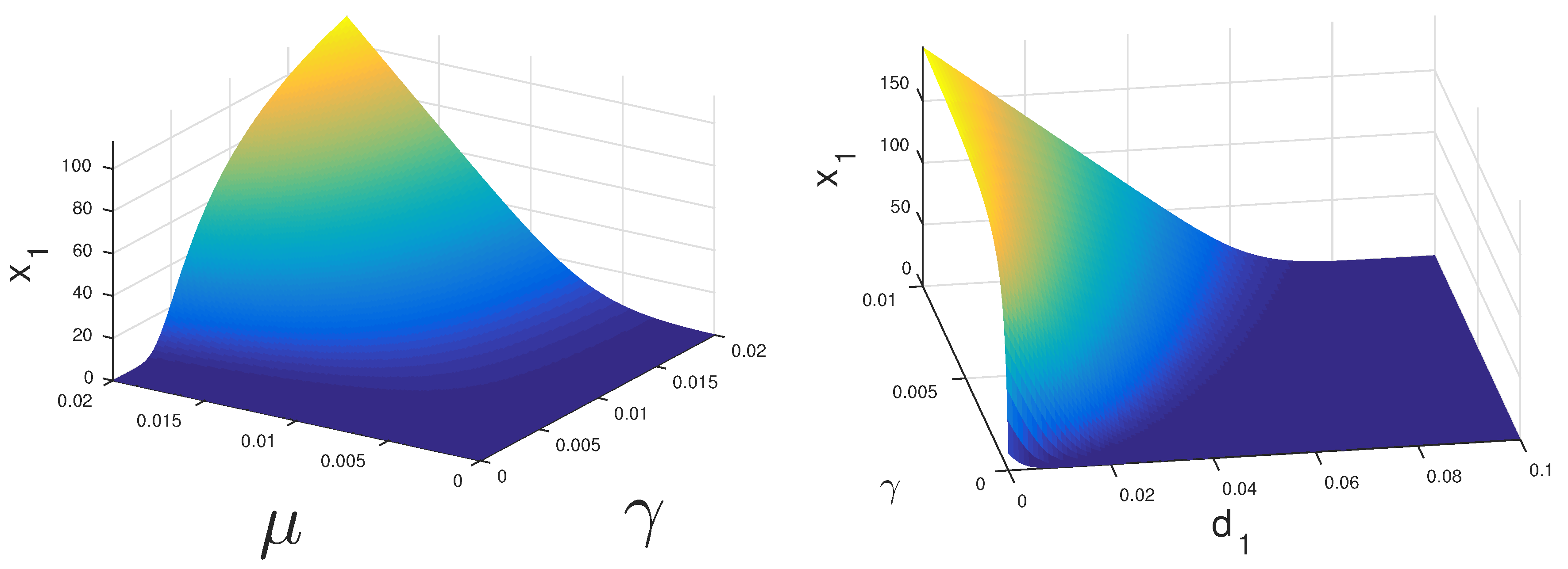
If both CS and CI cells can proliferate under treatment, then the coexistence equilibrium may be stable.
Figure 2 displays the regions where this could happen. If CS cells have a high growth rate
they may survive under relatively low levels of androgen. Alternatively, if these cells have a very low death rate
they may persist as well.
5. Parameter Estimation
In order to perform realistic model simulations, we need to obtain reasonable parameter values and their ranges. We start by estimating the realistic ranges for each of them. Parameters
μ,
,
are taken from [
33], where they assess the growth and death rates of prostate cells under different concentrations of androgen. In [
12], it was shown that, under continuous treatment, the fastest resistance rate is
. The approximate levels at which sensitive and resistant cells proliferate was studied in [
34], from which we approximated
q,
, and
.
In patients with no prostate cancer, PSA levels are usually less than 5
accounting for benign tumor hyperplasia [
8]. This implies that when tumor volume is near zero, the steady state of PSA given by:
shall be approximately 5
. Prostate tumor volumes are normally bounded by 80 mm in length and, on average, they are about
mm [
31]. Since all of our patients have advanced prostate cancer, we assumed a maximum length of 40 mm, and we compute the corresponding tumor volume assuming that tumors are spherical. Under complete androgen independence, tumor volume should not exceed 700
. Thus,
. Parameter
is patient specific and is taken from the maximum androgen serum concentration of each patient during the first 1.5 cycles of treatment. Parameter
is held constant among every patient and
has a range of 0–0.01
. The half-saturation variables
, and
are estimated from [
28].
Table 1 shows definitions, ranges, units, and sources for each of the parameters in our models.
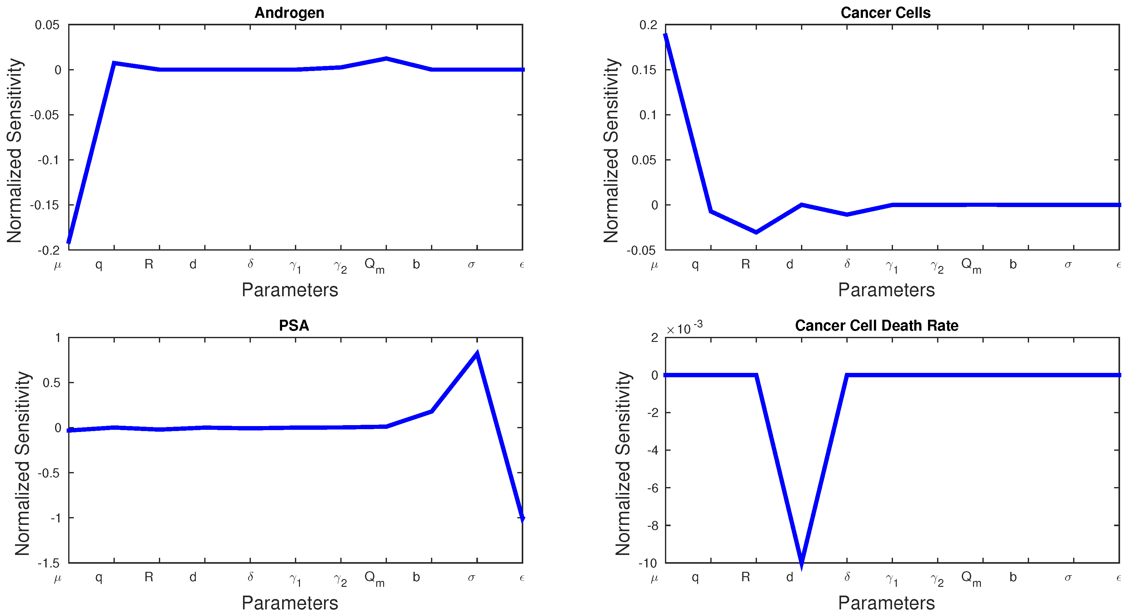
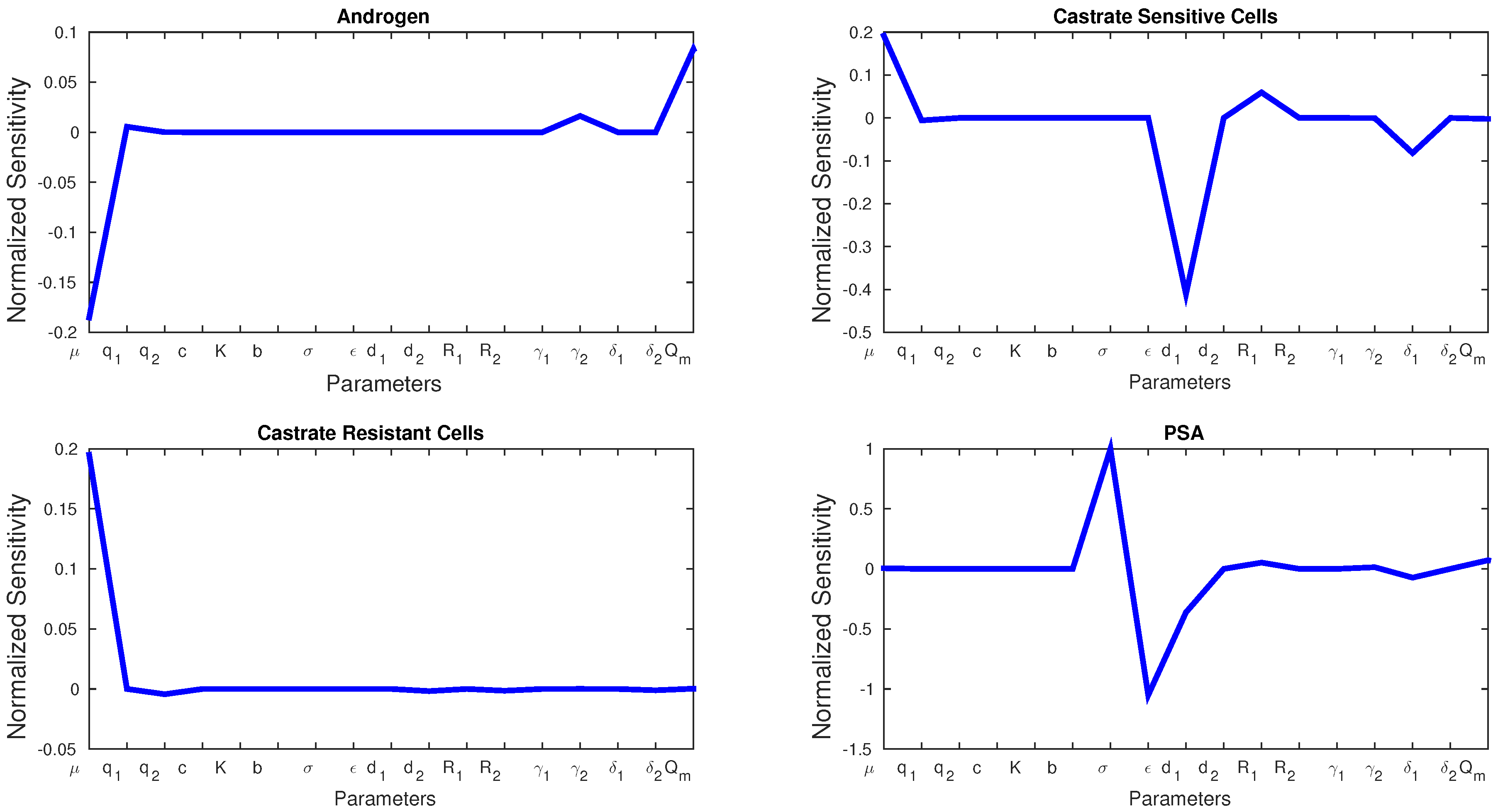
5.1. Sensitivity Analysis
Sensitivity analysis can be used to show which parameters play a bigger role in a model. The normalized sensitivity,
, for parameter
p and state variable
x is given by:
Figure 3 shows the sensitivities of every parameter and state variable for Model 1. We observe that, with the exception of
d, no parameter has a much larger sensitivity than the rest.
d is the only parameter that can dramatically affect cancer cell death rate, and we see a spike in the sensitivity figures. Cancer cell growth rate
μ has the greatest effect on androgen and cancer cells, whereas
σ and
ϵ play the greatest roles in PSA production.
Figure 4 shows the sensitivity of each parameter in Model 2. We see similarities with Model 1 in that
μ affects the production androgen and CR cells the most. In addition, PSA production is affected by the same parameters as in Model 1. Notice that CS cells are affected by
the most since they are the most susceptible to changes in the androgen concentration.
6. Comparison of Models
We use data from the Vancouver Prostate Center (Vancouver, BC, Canada) to validate and compare the accuracy of each model. From the 109 patients registered, 103 were eligible for interruption of treatment, with a PSA response rate of 95% [
9]. Using the criteria of having at least 20 data points for both androgen and PSA in the initial 1.5 cycles, we select 62 from those 109 patients. The individual PSA and androgen mean square error (MSE) are provided in
Table 2 from these 62 selected patients. Notice that the PKN model did not include an androgen equation, and thus we cannot compare the fittings of androgen with the PKN model.
For the PKN model, we interpolated androgen serum data using a cubic spline interpolation between every androgen data point. This created a function in terms of time that was utilized as
A in (13) and (14). We implemented the method used by Portz et al. [
13] for generating future androgen levels by generating a rectangular function based on the average off and on-treatment serum androgen values. Parameter ranges were taken from PKN [
13] and Everett et al. [
28], and the reader is referred to these papers for more details on forecasting serum PSA levels and parameter values of the PKN model. For every patient selected, we fitted 1.5 cycles of treatment and performed parameter estimation. Then, to measure the forecasting ability of every model, we ran the models for one more cycle of data using the parameters estimated from the initial 1.5 cycles.
To compare models, we conduct simulations with MATLAB’s (MATLAB 9.1, The MathWorks, Inc., Natick, MA, USA) built in function fmincon, which uses the Interior Point Algorithm, to find the optimum parameters for each patient. The algorithm searches for a minimum value in a range of pre-specified parameter ranges, which we estimated from various literature sources. We use this algorithm to minimize the MSE for PSA and androgen data. The MSE is calculated with the following equations:
where
N represents the total number of data points,
represents the PSA data value, and
the value from the model. Likewise,
represents the androgen data value, and
the value from the model. We then use an equally weighted combination of both errors
as our objective function, which is then minimized with fmincon.
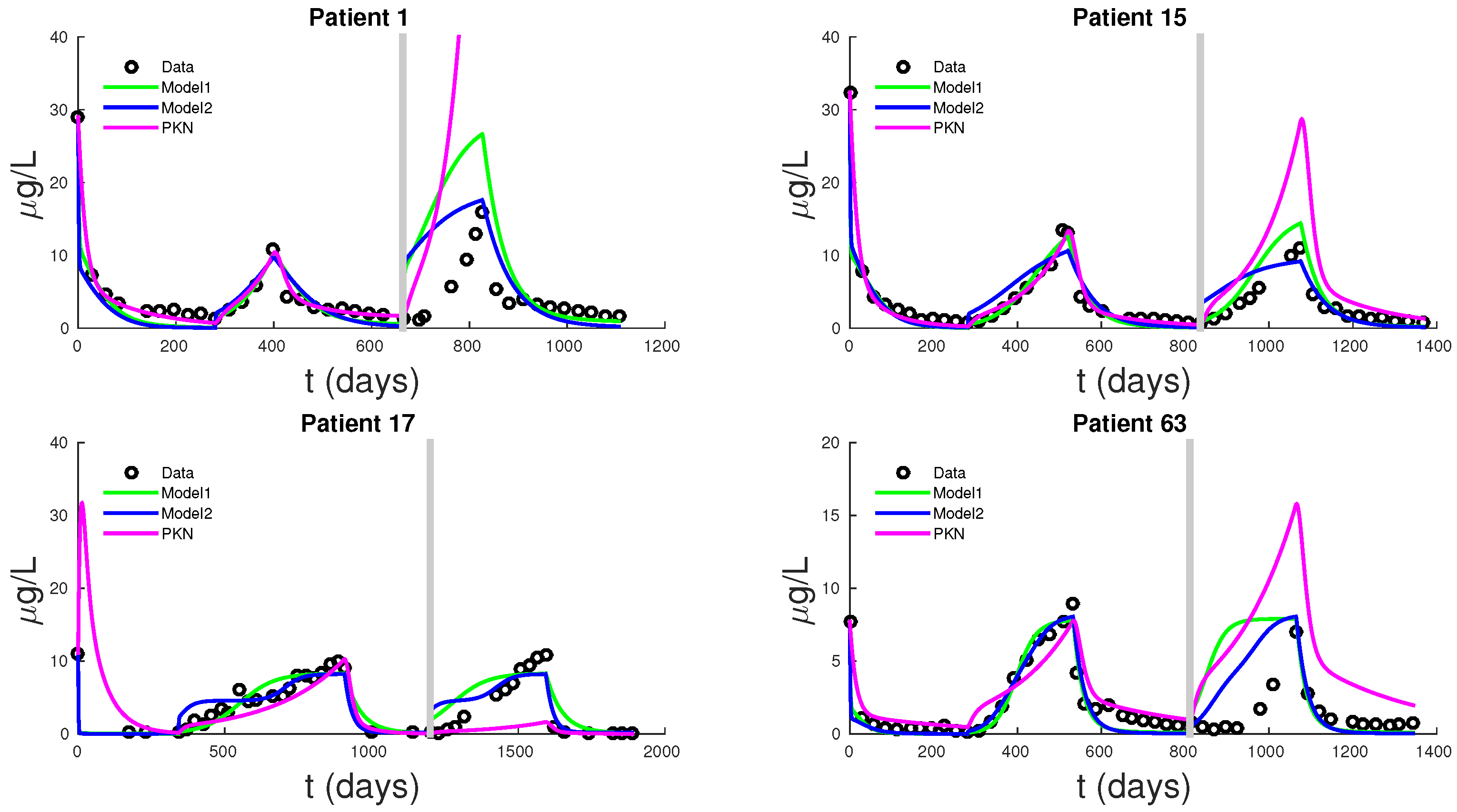
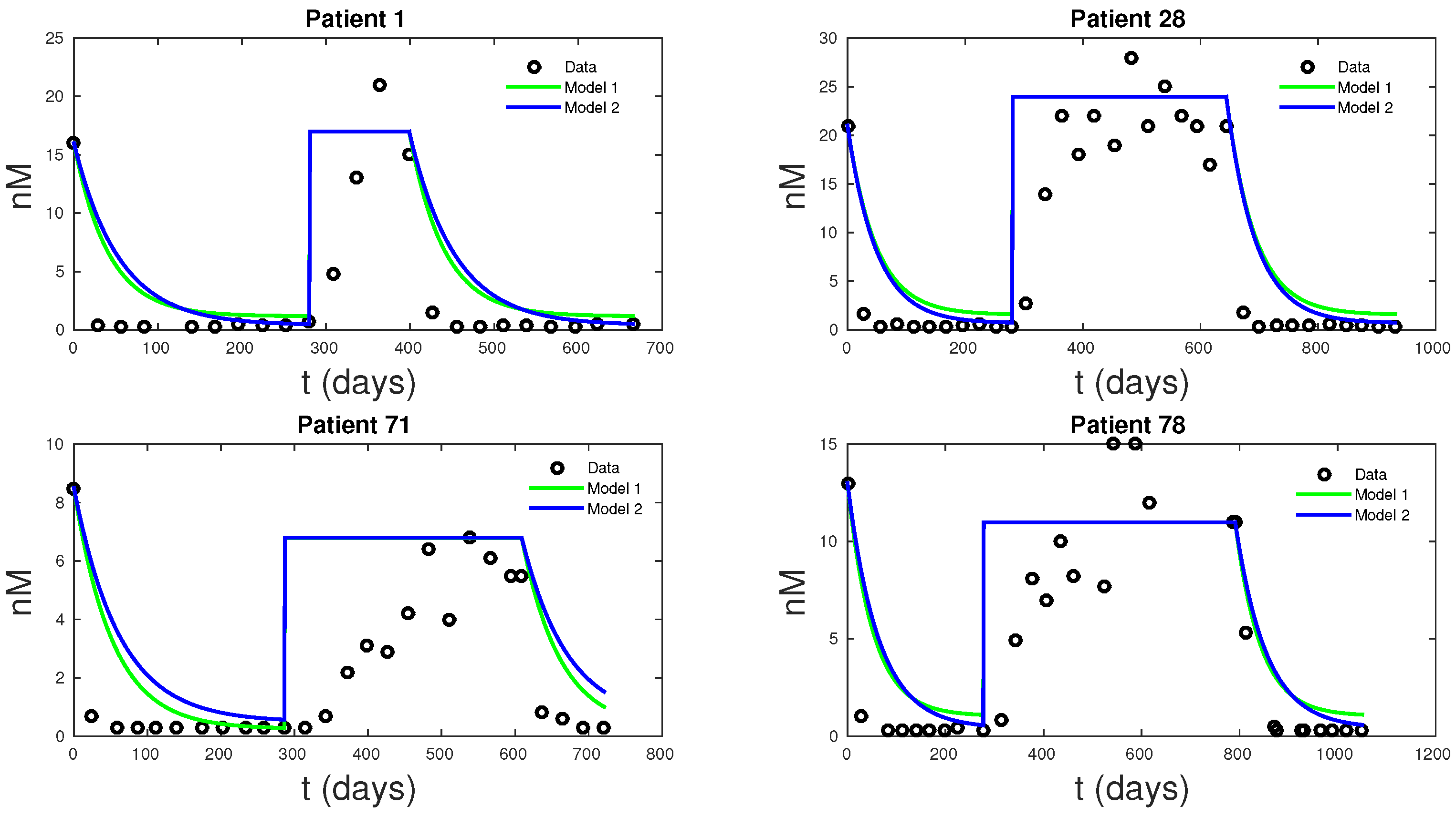
Figure 5 shows PSA fitting and forecasting simulations for patients 1, 15, 17, and 63. We selected these patients to display the typical behavior shown in all 62 patients. Patient 1 shows that Models 1, 2, and PKN fit data with about the same accuracy. However, PKN overshoots in forecasting and Model 2 outperforms Model 1 in forecasting. Patient 17 shows that PKN underestimates future PSA levels, but Models 1 and 2 both perform well. Patients 15 and 63 provide the cases where PKN does a better forecast while Models 1 and 2 still do better. The rest of the patients can be classified similarly.
Table 2 documents the error of fitting 1.5 cycles of treatment and
Table 3 displays the errors in forecasting one more cycle of treatment. On average, PKN and Model 1 perform prediction at the same level of accuracy. However, Model 2 performs prediction on average about three times better than the PKN model and Model 1.
7. Conclusions
The main goal of this research is to produce a basic model capable of describing prostate cancer cell growth subject to IAS. Such a model may be amendable to detailed and systematical mathematical and computational study aimed at revealing the near term and intermediate term growth dynamics, including cancer cells treatment resistance development. Ultimately, such models may be helpful in establishing user-friendly treatment tools for both patients and physicians. To this end, we presented two models that can accurately fit clinical PSA and androgen data simultaneously. Existing models can only fit the PSA data. While these models are simplifications of PKN, they are just as accurate in data fitting and even better at forecasting future PSA levels. Model 1 had the lowest mean MSE for data fitting of all the models, followed by PKN and Model 2—not surprisingly, due to its more biologically realistic model assumptions, Model 2 had the lowest forecast MSE, with PKN doing the worst. The unreliability of PKN’s forecasts stems from its dependence on androgen data and hence lacks the ability to predict androgen dynamics. Androgen cell quota values, which are not directly measurable from data, represent a significant source of uncertainty for the PKN model.
Figure 6, shows how the new models can fit clinical androgen data and reduce uncertainty. For Models 1 and 2,
Q is directly computable from clinical data.
Predicting the timing of resistance is a highly desirable objective of this modeling work. Mathematical models alone can not make practical predictions. However, we can use these models and apply statistical methods to produce reliable forecasts with confidence intervals [
35,
36]. In Pell et al. [
35] and Chowell et al. [
36], the authors have used these methods successfully in an epidemiological setting to make predictions. In a future paper, the authors plan to use the models presented in this paper to produce predictions using such statistical methods. Therefore, the main biological contribution of this work is the development of a clear and basic androgen cell-quota based model to aid our understanding of the resistance development dynamics of prostate cancer cells.
The dynamics of Model 1 is characterized by globally stable steady states. The mathematical analysis of Model 2 is only partially tractable. In fact, the stability and global stability of the cancer cell coexistence steady state remain unsettled. However, with our bifurcation analysis, we observe that under ADT or IAS,
cells may drive
cells to extinction. In
Figure 2, we see that with lower and realistic levels of androgen production when the patient is under ADT,
cells will eventually become extinct even at a higher level of proliferation compared to
cells. Thus, we concluded that, under continuous treatment, almost all patients will eventually become androgen resistant. However, it is still not clear if IAS delays the speed at which this occurs. With the models presented in this work, we have moved closer to the ultimate goal of modeling the androgen resistance of prostate cancer.
Our work is limited by the small number of patients considered. We selected 62 patients that had at least 20 data points in the first 1.5 cycles of treatment. Using a larger time interval and more patients to calibrate models might reveal more subtle differences in the models’ ability to fit data. Additionally, tumor volume data will allow us to validate the model more naturally.
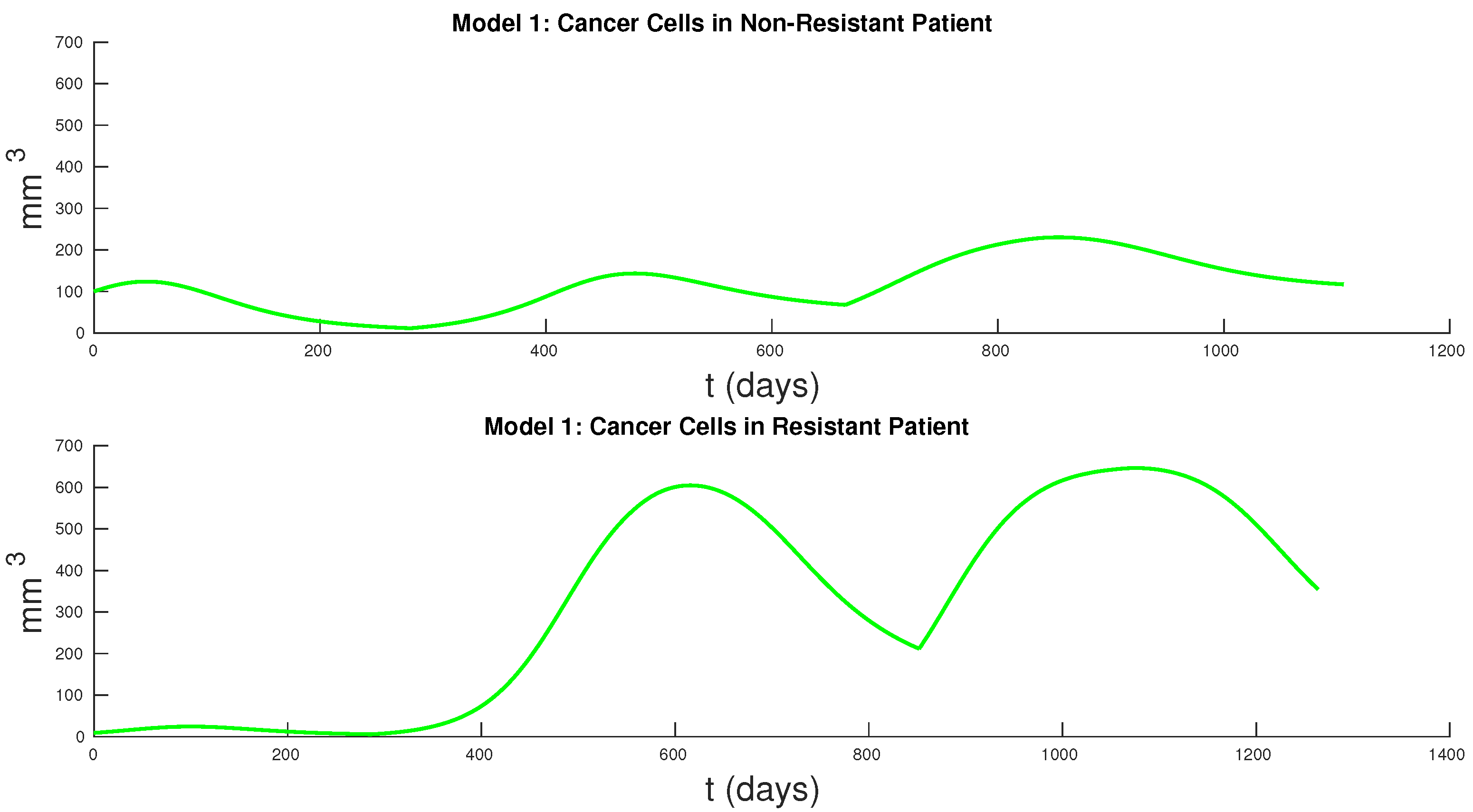
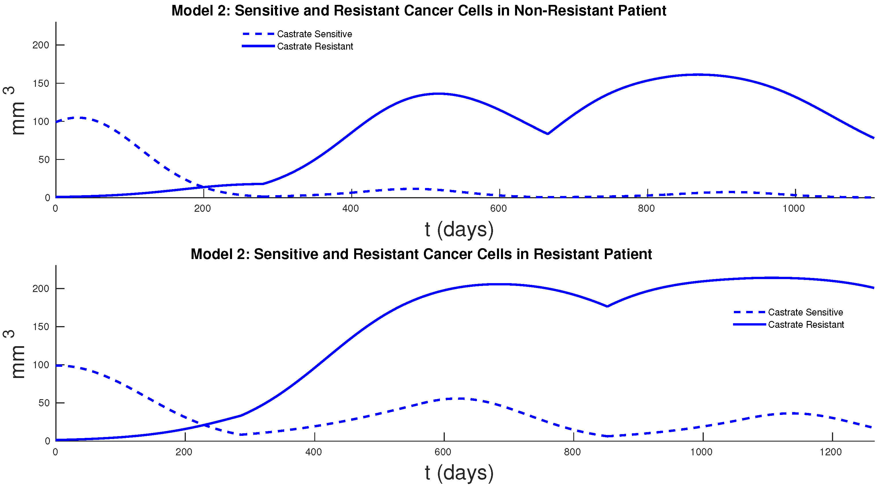
Figure 7 and
Figure 8 show the cancer populations for Models 1 and 2 in resistant and non-resistant patients. Tumor volume data will allow us to verify the results in these figures even if only a few data points are available.
In addition, identifiability analysis to determine if our parameter values can be represented uniquely by clinical data is essential if these models are to be used in a clinical setting to reliably and accurately predict PSA dynamics for individual patients. Allowing parameters to vary as treatment progresses and studying the changes in key parameter values such as proliferation and death rates as functions of time might be useful to describe and predict resistance mechanisms as suggested in the work of Morken et al. [
32].


