Article

Distributed Optimal Economic Dispatch Based on Multi-Agent System Framework in Combined Heat and Power Systems

Department of Electrical Engineering, Northeastern University, Shenyang 110819, China
*
Author to whom correspondence should be addressed.
Appl. Sci. 2016, 6(10), 308; https://doi.org/10.3390/app6100308
Submission received: 8 August 2016 / Revised: 26 September 2016 / Accepted: 14 October 2016 / Published: 23 October 2016

Abstract

:
In this paper, a novel distributed method is presented to solve combined heat and power economic dispatch problem, which is formulated as a distributed coupled optimization problem. The optimization goal is achieved by establishing two modified consensus protocols with two corresponding feedback parts while satisfying the electrical and heat supply–demand balance. Moreover, an alternating iterative method is proposed to handle the heat-electrical coupling problem existed in the objective function and the feasible operating regions. In addition, the proposed distributed method is implemented by a multi-agent system framework, which only requires local information exchange among neighboring agents. Simulation results obtained on a 16-bus test system are provided to illustrate the effectiveness of the proposed distributed method.

Graphical Abstract

1. Introduction

Economic dispatch, as one of fundamental and key problem in power system, is formulated to an optimization problem that aims at minimizing the total operating cost while satisfying the supply–demand balance constraint and some capacity limit. With pressures of energy crisis [1] and environment pollution [2,3], there is an increasing interest in utilizing combined heat and power (CHP) into the power system, to decrease carbon emission, increase energy efficiency, and save operational costs in recent years, which brings many challenges for the economic dispatch problem (EDP).
During these decades, there have been plentiful literature studies concerned with solving the combined heat and power economic dispatch problem (CHPEDP) in a centralized manner, such as the lambda iteration method [4], the gradient method [5], multi-team particle swarm optimization method [6], evolutionary method [7], etc. However, with the rapid development of the CHP system, centralized method has become the bottleneck of solving CHPEDP and cannot satisfy the requirement of practical applications. To be specific, the centralized methods have to rely on a central controller to communication with all the other system components to collect global information, resulting in great implementation cost and high sensitivity to single-point failures [8,9,10]. Moreover, both the physical and communication topology of the future CHP system are prone to have a huge and variable topology with partially-unknown characteristic, which may seriously degrade the effectiveness of centralized methods. In addition, each component in CHP system should possess the plug-and-play feature, which is one of the key characteristics of the future CHP system [11,12,13]. Thus, the centralized method is not very suitable to address the distributed features of the future CHP system.
The distributed methods featuring fast computation, high flexibility and reliability do not relay on the central controller and can provide cost-effective distributed solutions to meet the requirements of real-time application in modern power systems [14,15,16]. In fact, various distributed methods proposed only solve the EDP on the power grid side. For example, an incremental cost consensus method was proposed in [8] to solve the EDP in a distributed fashion, where a leader agent is needed to satisfy the electrical power balance constraint. In [17], a fully distributed method was proposed, in which the communication among generators are strongly connected and the estimation of power mismatch does not require a central controller or leader. Furthermore, the transmission losses, demand response and ramping rate limits have been taken into account and discussed in [18,19,20,21,22], respectively. In addition, there are also some researches analyzing the EDP from other perspectives, such as non-convex dispatch model [23], online generation adjustment [24], etc. It is worth noting that the aforementioned distributed methods are mainly focusing on the economic dispatch problem on the power side. However, there exist strong power-heat-coupling features both in the objective function and constraint limits in the CHP system scenario. Hence, the distributed methods above cannot apply to this kind of distributed coupling optimization problem.
Based on above discussions, this paper presents a novel distributed method to solve the CHPEDP. The proposed method is implemented based on two consensus procedure modified their corresponding feedback parts where the one is used to get the optimal electrical incremental cost and the other is used to get the optimal heat incremental cost, resulting in achieving the optimal solutions. Meanwhile, the alternating iterative method is proposed and used to solve the electrical–heat-coupling problem. In addition, the estimation of the electrical and heat power are also through distributed fashion, which are then used as a feedback mechanism to meet the supply–demand balance. The salient features of this paper are listed as follows:
(1) Various kinds of energy conversion devices fed by multiple-energy-carriers are modeled and considered to analyze the electrical and heat power production in CHP system, which can effectively increase the energy efficiency.
(2) The proposed method is fully distributed without a leader or central controller, which means it is more reliable and robust. In addition, the requirement on the communication topology of this paper is a strong connection that possesses less conservatism compared with undirected, connected communication topology.
(3) The CHPEDP has been formulated into a class of coupling optimization problem, which can be effectively solved by the proposed method in a distributed fully fashion. To the best knowledge of the authors, there still exist very few papers concerned about solving the CHPEDP in a distributed manner.
The rest of this paper is organized as follows. In Section 2, typical structure of CHP system, agent definitions and modeling are introduced. Then, the centralized method to solve the CHPEDP is discussed. In Section 3, some basic knowledge is briefly introduced, and the proposed distributed method is presented. In Section 4, several case studies are presented to show the effectiveness of the proposed method. Section 5 concludes the paper.

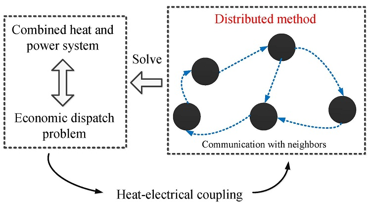
2. Problem Formulation

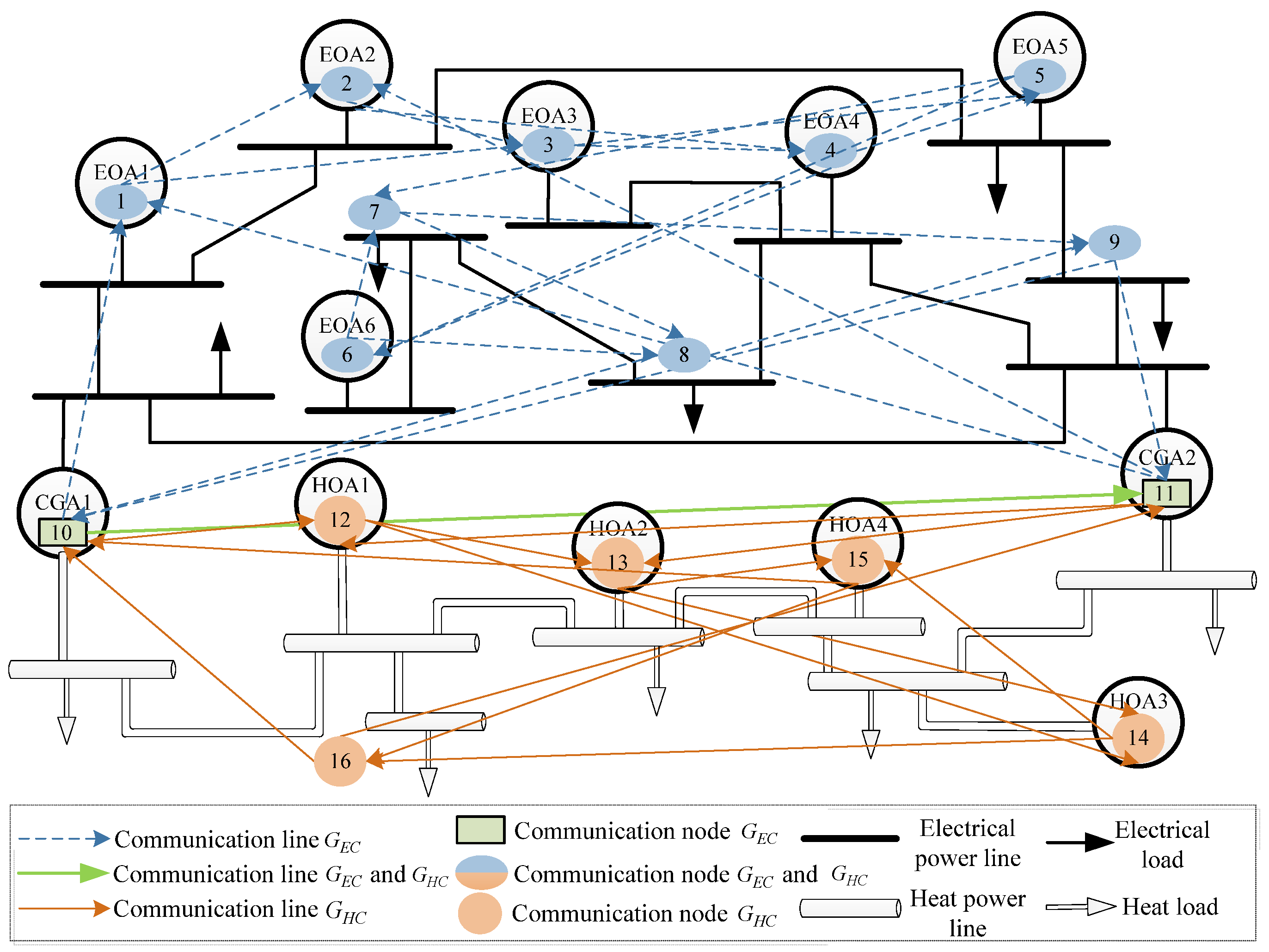
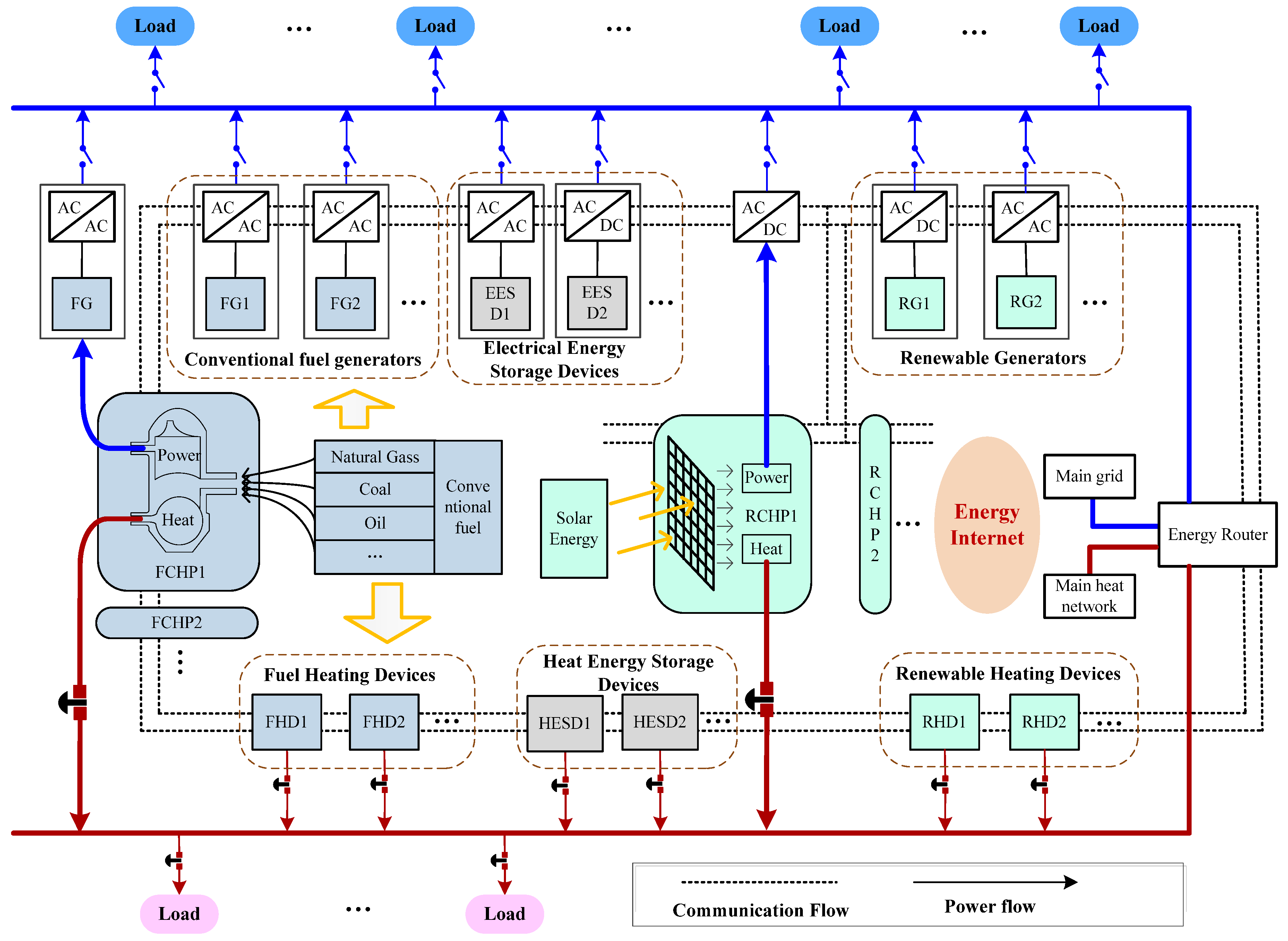
2.1. Structure and Agent Definitions
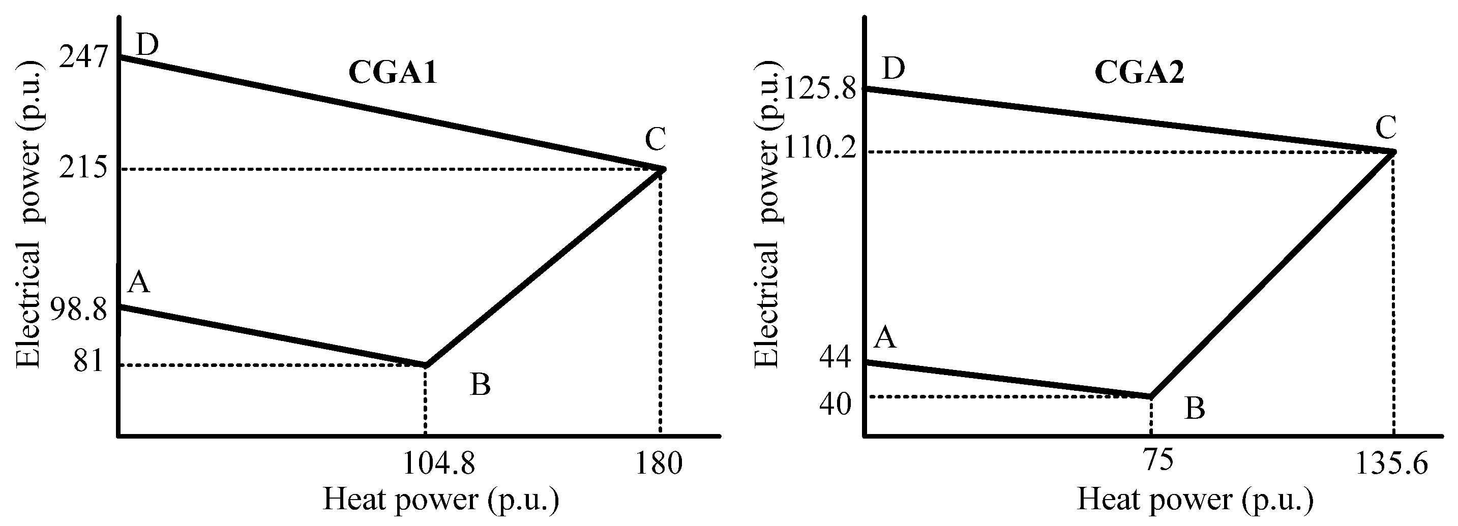
A typical architecture of CHP system is shown in Figure 1. Fed by multiple-energy-carriers, the energy resources of the CHP system consist of available distributed generators (DGs) that contain renewable generators (RGs) and fuel generators (FGs), distributed heating devices (DHDs) that contain renewable heating devices (RHDs) and conventional fuel heating devices (FHDs), distributed energy storage devices (DESDs) that contain electrical energy storage devices (EESDs) and heat energy storage devices (HESDs), CHPs that contain renewable combined heat and power (RCHP) and conventional fuel combined heat and power (FCHP), and loads that contain electrical loads and heat loads.
It is worth noting that the energy resources discussed above may generate different types of energy (electric and/or heat) power. To facilitate the system modeling, three types of agents are defined in this paper according to different energy power generation types. The three different agents include electricity–only agents (EOAs), co–generation agents (CGAs) and heat–only agents (HOAs). Therein, the EOAs, which can generate electrical power only, consist of various kinds of DGs and EESDs. The CGAs, which can generate not only electrical power but also heat power, consist of various kinds of CHPs. The HOAs, which can generate heat power only, consist of various kinds of DHDs and HESDs. Then, each type of agent will be formulated to build the system model in the next section.

2.2. Modeling

The cost function for CGAs is often modeled as the following form [6]:
C c i ( x i p q , x i q p ) = a i ( x i p q ) 2 + b i x p q + α i ( x i q p ) 2 + β i x i q p + γ i + ξ i x i p q x i q p
The feasible operating region for electrical and heat power output of a CGA is show in Figure 2. The region of ABCD denotes the bounds of the feasible operating region, which can be represented as a set of linear constraints, i.e., d m x p q + e m x q p + f m 0 ( m = 1 , 2 , 3 , 4 ). Furthermore, the set of linear constraints can be re-written as the following forms [4]:
x i _ min p q ( x i q p ) x i p q x i _ max p q ( x i q p )
x i _ min q p ( x i p q ) x i q p x i _ max q p ( x i p q )
The reasons for obtaining Equations (1b) and (1c) are as follows. For each feasible operation point ( x p q , x q p ) , we can get x p q ( e m x q p + f m ) / d m . Note that there always exist one (or several) e m / d m 0 and one (or several) e m / d m < 0 for different m. Thus, x p q ( e m x q p + f m ) / d m can be re-written as the form F max ( x q p ) x p q F min ( x q p ) . Therein, F min ( x q p ) and F max ( x q p ) , which are determined by x q p , are the upper and lower bound functions of x p q . In this paper, we define x min p q ( x q p ) and x max p q ( x q p ) as F min ( x q p ) and F max ( x q p ) , respectively. Similarly, we can define x min q p ( x p q ) and x max q p ( x p q ) as the lower and upper bound functions of x p q , respectively. Therefore, the expression of d m x p q + e m x q p + f m 0 is equivalent to the expressions of Equations (1b) and (1c).
The cost function of EOAs are modeled as the following form [25]:
C e i ( x i p ) = a i ( x i p ) 2 + b i x i p + γ i
x i _ min p x i p x i _ max p  
where b i and c i are both equal to zero for each EESD. Emphatically, x i _ max p = min { x i _ M P P T _ max p , x i _ w _ max p } of RG i are not constants, i.e., the maximum electrical power output of each wind generator will be changed following the change of wind speed.
The cost function of HOAs can also be modeled as the following form:
C h i ( x i q ) = α i ( x i q ) 2 + β j x i q + γ i
x i _ min q x i q x i _ max q
where β i and γ i are both equal to zero for every HESD. Similarly, for RHDs, x i _ max q = min { x i _ M P P T _ max q , x i _ w _ max q } .
The CHPEDP is to coordinate all the agents to minimize the system production cost C ( x ) while the electrical and heat power balance constraints, and a set of capacity limits constraints are satisfied. The objective can be mathematically represented as follows:
C ( x ) = i = 1 n 1 C e i ( x i p ) + i = n 1 + 1 n 1 + n 2 C c i ( x i p q , x i q p ) + i = n 1 + n 2 + 1 n 1 + n 2 + n 3 C h i ( x i q )
subject to
i = 1 n 1 x i p + i = n 1 + 1 n 1 + n 2 x i p q D P = 0
i = n 1 + 1 n 1 + n 2 x i q p + i = n 1 + n 2 + 1 n 1 + n 2 + n 3 x i q D Q = 0
and Equations (1b), (1c), (2b) and (3b).
In this paper, when i = 1 , , n 1 , it expresses the EOA. Similarly, when i = n 1 + 1 , , n 1 + n 2 and i = n 1 + n 2 + 1 , , n 1 + n 2 + n 3 , it expresses the CGA and HOA, respectively.

2.3. Centralized Method

The Lagrange multiplier theory can be used to analyze the CHPEDP. Inspired by the Lagrange multiplier theory, a fully distributed method will be introduced in Section 3. The Lagrange function is expressed as following equation:
L = C ( x ) λ p ( i = 1 n 1 x i p + i = n 1 + 1 n 1 + n 2 x i p q D P ) λ q ( i = n 1 + 1 n 1 + n 2 x i q p + i = n 1 + n 2 + 1 n 1 + n 2 + n 3 x i q D Q ) μ i _ min ( x i x i _ min ) μ i _ max ( x i _ max x i )
When the inequality constraints are not taken into account, the Lagrangian operator provides the following set of equations:
{ L x i p = 2 a i x i p + b i λ p = 0 ,    L x i p q = 2 a i x i p q + b i + ξ i x i q p λ p = 0 L x i q p = 2 α i x i q p + β i + ξ i x i p q λ q = 0 ,    L x i q = 2 α i x i q + β i λ q = 0
Let C e i ( x i p ) / x i p = 2 a i x i p + b i and C c i ( x i p q , x i q p ) / x i p q = 2 a i x i p q + b i + ξ i x i q p be the electrical incremental cost, and C c i ( x i p q , x i q p ) / x i q p = 2 α i x i q p + β i + ξ i x i p q and C h i ( x i q ) / x i q = 2 α i x i q + β i be the heat incremental cost. According to Equation (7), the necessary conditions of the existing optimal operating point are that the entire electrical incremental cost and the heat incremental cost must be equal to λ p and λ q , respectively. If there exists the optimal operating point, the calculations of the electrical and heat power are given by:
{ x i p = ( λ p * b i ) / 2 a i , x i p q = ( λ p * b i ξ i x i q p ) / 2 a i x i q p = ( λ q * β i ξ i x i p q ) / 2 α i , x i q = ( λ q * β i ) / 2 α i
Furthermore, when the inequality constraints are taken into account, the necessary conditions to solve the problem can be expanded as:
{ C i / x i = λ ν * , x i _ min < x i < x i _ max C i / x i λ ν * , x i _ max = x i C i / x i λ ν * , x i _ min = x i
where if = p , λ ν * , x i _ min and x i _ max denote λ p * , x i _ min p and x i _ max p , respectively. If = p q , λ ν * , x i _ min and x i _ max denote λ p * , x i _ min p q ( x i q p ) and x i _ max p q ( x i q p ) , respectively. If = q p , λ ν * , x i _ min and x i _ max denote λ q * , x i _ min q p ( x i p q ) and x i _ max q p ( x i p q ) , respectively. If = q , λ ν * , x i _ min and x i _ max denote λ q * , x i _ min q and x i _ max q , respectively.
Remark 1:
Compared with the distributed methods [8,17,18,19,20,21,22,23,24], in CHP system, the relationship between electrical and heat power are coupled, which existed in the objective function caused by the nonzero coefficient ξ i of Equation (1a), and in the feasible operating region of CGAs mathematically represented as Equations (1b) and (1c). The former results in the calculation of x i p q ( x i q p ) depend on not only λ p * ( λ q * ) but also x i q p ( x i p q ), as shown in Equation (8). The latter expresses that the lower and upper bounds of x i p q ( x i q p ) are not two constants but turning to two different functions which collectively depend on x i p q and x i q p as shown in Equation (9). Thus, the optimal solutions cannot be separately calculated by the power system or heat system.

3. Distributed Method

3.1. Basic Knowledge

(1) Graph Theory: A weighted directed graph G = ( V , E ) is composed of a set of nodes V = ( v 1 , v 2 , , v n ) and a set of arcs E = { e i j = ( v i , v j ) } V × V . Therein, the i th agent can receive information from j th agent if the corresponding arc e i j exists. If agent i can get (send) information from (to) agent j , then agent j is called in-neighbors (out-neighbors) of agent i . The set of in-neighbors (out-neighbors) is denoted by N i i n ( N i o u t ) with cardinality d i i n ( d i o u t ). It is assumed that every agent has self-loops, which means every agent can send and receive information to itself. An undirected graph is connected if there exists an undirected path between any pairs of distinct nodes. A directed graph is strongly connected if there exists a path between any pair of two nodes with respect to the orientation of arcs. A nonnegative matrix is called row (or column) stochastic if all of its row-sums (or column-sums) are 1. In this paper, graph nodes represent the agents, and the graph arcs represent the communication links among agents.
(2) Basic Definitions: Consider a CHP system G with n 1 EOAs, n 2 CGAs and n 3 HOAs. Let the CHP system include two subgraphs G E C and G H C , where G E C composed of EOAs and CGAs, and G H C composed of HOAs and CGAs, meanwhile the two subgraphs are both strongly connected digraphs. Moreover, define two matrices R , S in subgraph G E C , where R is row stochastic and S is column stochastic. Let r i , j = 1 / d i i n if j N i i n , r i , j = 0 if j N i i n , and s i , j = 1 / d j o u t if i N j o u t , s i , j = 0 if i N j o u t . Similarly, define two matrices R ¯ and S ¯ in subgraph G H C , where R ¯ is row stochastic and S ¯ is column stochastic. Let r ¯ i , j = 1 / d ¯ i i n if j N ¯ i i n , r ¯ i , j = 0 if j N ¯ i i n , and s ¯ i , j = 1 / d ¯ j o u t if i N ¯ j o u t , s ¯ i , j = 0 if i N ¯ j o u t .
(3) Consensus algorithm (or protocol): Based on the definitions discussed above, the first-order consensus protocol is given by:
χ i ( t + 1 ) = j N i n r i , j χ j ( t )
Since R is row stochastic, Equation (10) forms the first-order consensus protocol [26]. Each agent reaches the final common value χ i ( ) = ω T χ ( 0 ) .

3.2. Distributed Method

Inspired by the consensus algorithm, this paper focuses on combing the consensus algorithm and the optimization theory to design a suitable, distributed method to solve the CHPEDP. Therein, there exist strong power-heat-coupling features both in the objective function and constraint limits. To address this issue, from the analysis in Section 2.3, there is not only an optimal electrical incremental cost λ p * but also an optimal heat incremental cost λ q * . More importantly, λ p * and λ q * are global variables. However, there is no centralized controller in this paper. Thus, the basic concept is to establish two different consensus protocols, in which the one is to make the electrical incremental cost run an common value (i.e., the final consensus value) and the other is to make heat incremental cost run an another common value, meanwhile a feedback mechanism is designed and added into the corresponding consensus protocol to obtain the optimal λ p * and λ q * . In addition, to solve the electrical–heating-coupling problem, which has been illustrated in Remark 1, the basic idea is to establish an effective alternating iterative method to solve this problem, where electricity and heat alternately converge to the optimal solution. Then, the updating rules of the proposed distributed method are designed as:
(1) In the even-numbered iteration
{ λ i p ( 2 k ) = λ i p ( 2 k 1 ) , λ i p q ( 2 k ) = λ i p q ( 2 k 1 ) λ i q p ( 2 k ) = j N ¯ i i n r ¯ i , j λ j ϑ ( 2 k 1 ) + η y i q p ( 2 k 1 ) , λ i q ( 2 k ) = j N ¯ i i n r ¯ i , j λ j ϑ ( 2 k 1 ) + η y i q ( 2 k 1 )
{ z i p ( 2 k ) = x i p ( 2 k 1 ) , z i p q ( 2 k ) = x i p q ( 2 k 1 ) z i q p ( 2 k ) = ( λ i q p ( 2 k ) β i ξ i x i p q ( 2 k 1 ) ) / 2 α i , z i q ( 2 k ) = ( λ i q ( 2 k ) β i ) / 2 α i
{ x i p ( 2 k ) = z i p ( 2 k ) , x i p q ( 2 k ) = z i p q ( 2 k ) x i q p ( 2 k ) = { z i _ min q p ( 2 k ) ( z i p q ( 2 k ) ) i f z i q p ( 2 k ) < z i _ min q p ( 2 k ) ( z i p q ( 2 k ) ) z i _ max q p ( 2 k ) ( z i p q ( 2 k ) ) i f z i q p ( 2 k ) > z i _ max q p ( 2 k ) ( z i p q ( 2 k ) ) z i q p ( 2 k ) otherwise , x i q ( 2 k ) = { x i _ min q i f z i q ( 2 k ) < x i _ min q x i _ max q i f z i q ( 2 k ) > x i _ max q z i q ( 2 k ) otherwise
{ y i p ( 2 k ) = y i p ( 2 k 1 ) , y i p q ( 2 k ) = y i p q ( 2 k 1 ) y i q p ( 2 k ) = j N ¯ i o u t s ¯ i , j y j ϑ ( 2 k 1 ) x i q p ( 2 k ) + x i q p ( 2 k 1 ) y i q ( 2 k ) = j N ¯ i o u t s ¯ i , j y j ϑ ( 2 k 1 ) x i q ( 2 k ) + x i q ( 2 k 1 )
(2) In the odd-numbered iteration
{ λ i p ( 2 k + 1 ) = j N i i n r i , j λ j θ ( 2 k ) + η y i p ( 2 k ) , λ i p q ( 2 k + 1 ) = j N i i n r i , j λ j θ ( 2 k ) + η y i p q ( 2 k ) λ i q p ( 2 k + 1 ) = λ i q p ( 2 k ) , λ i q ( 2 k + 1 ) = λ i q ( 2 k )
{ z i p ( 2 k + 1 ) = ( λ i p ( 2 k + 1 ) b i ) / 2 a i , z i p q ( 2 k + 1 ) = ( λ i p q ( 2 k + 1 ) b i ξ i x i q p ( 2 k ) ) / 2 a i z i q p ( 2 k + 1 ) = x i q p ( 2 k ) , z i q ( 2 k + 1 ) = x i q ( 2 k )
{ x i p ( 2 k + 1 ) = { x i _ min p i f z i p ( 2 k + 1 ) < x i _ min p x i _ max p i f z i p ( 2 k + 1 ) > x i _ max p z i p ( 2 k + 1 ) otherwise , x i p q ( 2 k + 1 ) = { z i _ min p q ( 2 k + 1 ) ( z i q p ( 2 k + 1 ) ) i f z i p q ( 2 k + 1 ) < z i _ min p q ( 2 k + 1 ) ( z i q p ( 2 k + 1 ) ) z i _ max p q ( 2 k + 1 ) ( z i q p ( 2 k + 1 ) ) i f z i p q ( 2 k + 1 ) > z i _ max p q ( 2 k + 1 ) ( z i q p ( 2 k + 1 ) ) z i p q ( 2 k + 1 ) otherwise x i q p ( 2 k + 1 ) = z i q p ( 2 k + 1 ) , x i q ( 2 k + 1 ) = z i q ( 2 k + 1 )
{ y i p ( 2 k + 1 ) = j N i o u t s i , j y j θ ( 2 k ) x i p ( 2 k + 1 ) + x i p ( 2 k ) y i p q ( 2 k + 1 ) = j N i o u t s i , j y j θ ( 2 k ) x i p q ( 2 k + 1 ) + x i p q ( 2 k ) y i q p ( 2 k + 1 ) = y i q p ( 2 k ) , y i q ( 2 k + 1 ) = y i q ( 2 k )
where θ denotes p or p q , ϑ denotes q p or q , and t = 2 k or 2 k + 1 . In addition, we let Φ = [ λ i θ , z i θ , x i θ , y i θ ] ( Θ = [ λ i ϑ , z i ϑ , x i ϑ , y i ϑ ] ) represent all the variables relating to heat (electrical) power.
Equation (11) shows the updating rules for Θ ( 2 k ) . In this step, the purpose is to make Θ go to the optimal solution, meanwhile Φ ( 2 k ) = Φ ( 2 k 1 ) so that they can be seen as unchanged for further updating Θ . The detailed updating processes are as the following statements. Firstly, λ i q p ( 2 k ) and λ i q ( 2 k ) in Equation (11a) compose to the first consensus protocol, which includes consensus part and feedback part. The consensus part is associated to row stochastic R ¯ which drives λ i q p ( 2 k ) and λ i q ( 2 k ) to a common value. The feedback part includes η y i q p ( 2 k 1 ) and η y i q ( 2 k 1 ) which can let HOAs and CGAs change their incremental cost to satisfy the electrical power supply–demand balance to further obtain the optimal λ q * . That is, each HOA or CGA decrease (or increase) its corresponding heat incremental cost and heat power output when y i q ( 2 k 1 ) or y i q p ( 2 k 1 ) is negative (or positive) for the common value further adjustment to λ q * . Secondly, according to Equation (8), z i q p ( 2 k ) and z i q ( 2 k ) in Equation (11b) are used to update the estimated heat power outputs before considering the inequality constraints. Then, according to Equation (9), Equation (11c) defines the projection operators to take account of the inequality constraints, on the basis of the first assumption that x i _ w _ min p q x i p q ( 2 k 1 ) x i _ w _ max p q must be satisfied. Finally, inspired by literature [21], y i q p ( 2 k ) and y i q ( 2 k ) in Equation (11d) are used to update the estimated the heat power mismatch in a fully distributed fashion, which will be used to adjust the heat power incremental cost in the next cycle.
Similarly, Equation (12) shows the updating rules for Φ ( 2 k + 1 ) meanwhile Θ ( 2 k + 1 ) = Θ ( 2 k ) . λ i p ( 2 k + 1 ) and λ i p q ( 2 k + 1 ) in Equation (12a) compose to the second modified consensus protocol which also includes its corresponding consensus part associated to row stochastic R and feedback part (i.e., η y i p ( 2 k ) and η y i p q ( 2 k ) ) to obtain the optimal λ p * . z i p ( 2 k + 1 ) , z i p q ( 2 k + 1 ) in Equation (12b) and x i p ( 2 k + 1 ) , x i p q ( 2 k + 1 ) in Equation (12c) are used to update the estimated electrical power outputs before and after considering the inequality constraints, respectively, on the basis of the second assumption x i _ w _ min q p x i q p ( 2 k ) x i _ w _ max q p . y i p ( 2 k + 1 ) and y i p q ( 2 k + 1 ) in Equation (12d) are used to update the estimated the electrical power mismatch.
According to the aforementioned statement, we can give the major conclusion as follows. If the studied problem (Equation (4)) is feasible, then the method composed of Equations (11a)−(11c) and (12a)−(12c) is stable. Furthermore, each variable can converge to its optimal value, i.e., λ i q λ q * , λ i q p λ q * , λ i p λ p * , λ i p q λ p * , x i q x i q * , x i q p x i q p * , x i p x i p * , x i p q x i p q * as t (he proof can be seen in Appendix A).
According to Remark 2, for each CGA, the initial values of electrical and heat power outputs, i.e., x i p q ( 0 ) and x i q p ( 0 ) , can be set to any values in the corresponding feasible operating region. For convenience, we set the value of point B ( x i _ B p q , x i _ B q p ) in Figure 2 as the initial value, i.e., x i p q ( 0 ) = x i _ B p q and x i q p ( 0 ) = x i _ B q p . In addition, if bus i has electrical or heat load only, then it can be assumed that there is a fictitious EOA (or HOA) with x i _ min p = x i _ max p = 0 (or x i _ min q = x i _ max q = 0 ). Then, for each EOA (or HOA), the initial value of electrical (or heat) power output, i.e., x i p ( 0 ) (or x i q ( 0 ) , can be any value. Furthermore, we set the corresponding lower bound as its initial value. The initial values of electrical and heat incremental costs, i.e., λ i p ( 0 ) , λ i p q ( 0 ) , λ i q p ( 0 ) and λ i q ( 0 ) , which can also be any values, are set as zeros in this paper. In addition, the initial electrical (or heat) power mismatches, i.e., y i p ( 0 ) and y i p q ( 0 ) (or y i q ( 0 ) and y i q p ( 0 ) , are set as the difference between the local electrical (or heat) load demands and the initial electrical (or heat) power outputs. To sum up, each variable is initialized as follows:
{ x i p ( 0 ) = x i _ min p , x i p q ( 0 ) = x i _ B p q , x i q p ( 0 ) = x i _ B q p , x i q ( 0 ) = x i _ min q λ i p ( 0 ) = λ i p q ( 0 ) = λ i q p ( 0 ) = λ i q ( 0 ) = 0 y i p ( 0 ) = L i _ E x i p ( 0 ) , y i p q ( 0 ) = L i _ E x i p q ( 0 ) , y i q p ( 0 ) = L i _ H x i q p ( 0 ) , y i q ( 0 ) = L i _ H x i q ( 0 )
Remark 2:
There are two assumptions which must be satisfied during the updating process. In the even-numbered iteration, we have x i p q ( 2 k 1 ) = z i p q ( 2 k ) = x i p q ( 2 k ) . Thus, if the first assumption x i _ w _ min p q x i p q ( 2 k 1 ) x i _ w _ max p q is satisfied, then x i _ w _ min p q z i p q ( 2 k ) x i _ w _ max p q which indicates ( z i p q ( 2 k ) , z i q p ( 2 k ) ) is within the area between L1 and L2 as shown in Figure 2. Due to the calculation of z i q p ( 2 k ) without considering the inequality constraints, ( z i p q ( 2 k ) , z i q p ( 2 k ) ) may be out of the feasible operating region, e.g., the point E shown in Figure 2. However, the upper and lower bounds of z i q p ( 2 k ) can be easily obtained, because z i p q ( 2 k ) is known. Then, by using the corresponding projection operator (11c), the infeasible point can be mapped into the feasible operating region to further obtain ( x i p q ( 2 k ) , x i q p ( 2 k ) ) , e.g., the point G shown in Figure 2. It is not very difficult to verify that x i q p ( 2 k ) satisfies x i _ w _ min q p x i q p ( 2 k ) x i _ w _ max q p . Thus, in the next iteration, the second assumption is satisfied. Then, ( z i p q ( 2 k + 1 ) , z i q p ( 2 k + 1 ) ) is within the area between L3 and L4. By using the projection operator 12(c), ( x i p q ( 2 k + 1 ) , x i q p ( 2 k + 1 ) ) can be further calculated, which is within the feasible operating region. By such analogy, the two assumptions will be always satisfied if only the initial value of ( x i p q ( 0 ) , x i q p ( 0 ) ) is in the feasible operating region.
For clarify, the proposed distributed method is summarized as:
Distributed Consensus-Based Method
Initialize: Each agent initializes all of variables based on Equation (13)
Iteration: ( t > 0 )
(1). 
Each agent exchanges the local information of λ i p , λ i p q , λ i q p and λ i q (and y i p , y i p q , y i q p and y i q ) with its neighbors.
(2). 
If t = 2 k (i.e., in the even-numbered iteration)
(2a). 
Update λ i p , λ i p q , λ i q p and λ i q based on Equation (11a)
(2b). 
Update z i p , z i p q , z i q p and z i q (i.e., the estimated electrical and heat power outputs before considering inequality constraints) based on Equation (11b)
(2c). 
Choose projection operations based on Equation (11c) to calculate x i p , x i p q , x i q p and x i q (i.e., the estimated electrical and heat power outputs after considering inequality constraints)
(2d). 
Update y i p , y i p q , y i q p and y i q based on Equation (11d)
(3). 
Else (i.e., in the odd-numbered iteration)
(3a). 
Update λ i p , λ i p q , λ i q p and λ i q based on Equation (12a)
(3b). 
Update z i p , z i p q , z i q p and z i q based on Equation (12b)
(3c). 
Choose projection operations based on Equation (12c) to calculate x i p , x i p q , x i q p and x i q
(3d). 
Update y i p , y i p q , y i q p and y i q based on Equation (12d)
(4). 
Let t = t + 1 , turn to step 1.
Remark 3:
The distributed fashion of our method is reflected in that each agent only requires its own information and neighbors’ information to calculate the optimal solution. Specifically, each agent only needs to exchange the local information of λ i p , λ i p q , λ i q p and λ i q (and y i p , y i p q , y i q p and y i q ) with its neighbors. Furthermore, the updating processes for all of variables are implemented through local calculation. On the contrary, centralized methods require a central controller and rely on a two-way communication network structure between the central controller and each agent. The central controller should collect all of the information of each agent to calculate the optimal solution, and then sent the optimal solution to each agent.
Remark 4:
Existing methods to solve the CHPEDP are mainly based on the centralized fashion, such as [4,7], etc. However, they have some obvious demerits as follows. (1) Since the centralized methods rely on a central controller, they are susceptible to single-point failures. To be specific, if the communication line between the central controller and any agent is failure, then the corresponding agent cannot keep working in the optimal operating point. Moreover, if the centralized controller is failure, then the whole system will lose control which may result in serious consequence, e.g., supply–demand unbalance. (2) When a new agent is connected to the system, the communication link between the new agent and the central controller must be established, which cannot be flexible for possible integration and expansions of devices. (3) Centralized methods cannot provide a satisfied plug-and-play function. On the contrary, the proposed distributed method is more reliable, robust, flexible and cost-effective and can address the plug-and-play feature in a better way. To be specific, since each agent can calculate its optimal operating point by using its own and neighbors information, a single (even several) link failures will not affect the optimal performance as long as the communication network maintains strong connection. Furthermore, when a new agent is required to be added into the system, the agent needs only establish the communication links with its neighbor agents, which simplifies the system maintenance and possible expansions. Moreover, the communication structure used in this paper with strong connection is a sparse communication structure, in which each agent only needs its local information and its neighbor’s information to calculate the optimal solution. Thus, distributed method used in this paper is less expensive and more cost-effective. In addition, the distributed method provides desired plug-and-play feature for the future CHP system. It is very difficult for centralized method to meet this feature when the system becomes larger and larger.
Remark 5:
According to the definitions in graph theory, it can be seen that strongly connected structure belongs to directed graph while connected structure belongs to undirected graph. This also means, under strongly connected structure, each agent can send information to or receive information from its neighbors through single-way communication network. However, if it is under connected structure in undirected graph, each agent must send information to and receive information from its neighbors in the same time through two-way communication network. In other words, the strongly connected structure requires only a single-way communication network while the connected structure requires a two-way communication network. Thus, the strongly connected topology possesses less conservatism compared with connected graph. In addition, it is well-known that the convergence analysis, in the field of distributed control, is much more challenging under the directed graph setting.

4. Simulation Results

The first case is used to show the effectiveness of the proposed method via comparing with the well-known Lagrangian relaxation method. In the second case, one-day load demand of Northeastern University is used to test the performance of the proposed method under time-varying demand. The third case shows the requirement of plug and play. The last case considers the change of the maximum peak power tracking point for RGs and RHDs. The physical and communication structure of the test system is shown in Figure 3, in which EOA1, -3 and -5 represent three different FGs, EOA2 represents a EESD, EOA4 and -6 represent two different RGs, CGA1 and -2 represent two different CHPDs, HOA1 and -2 represent two different FHDs, HOA3 represents a RHDs and HOA4 represents a HESD. The parameters of each agent are listed in Table 1. The feasible operating region of CGA1 and CGA2 are shown in Figure 4. In the first three cases, the maximum peak power tracking point for EOA4, EOA6 and HOA3 are 90 (p.u.), 130 (p.u.) and 180 (p.u.), respectively.

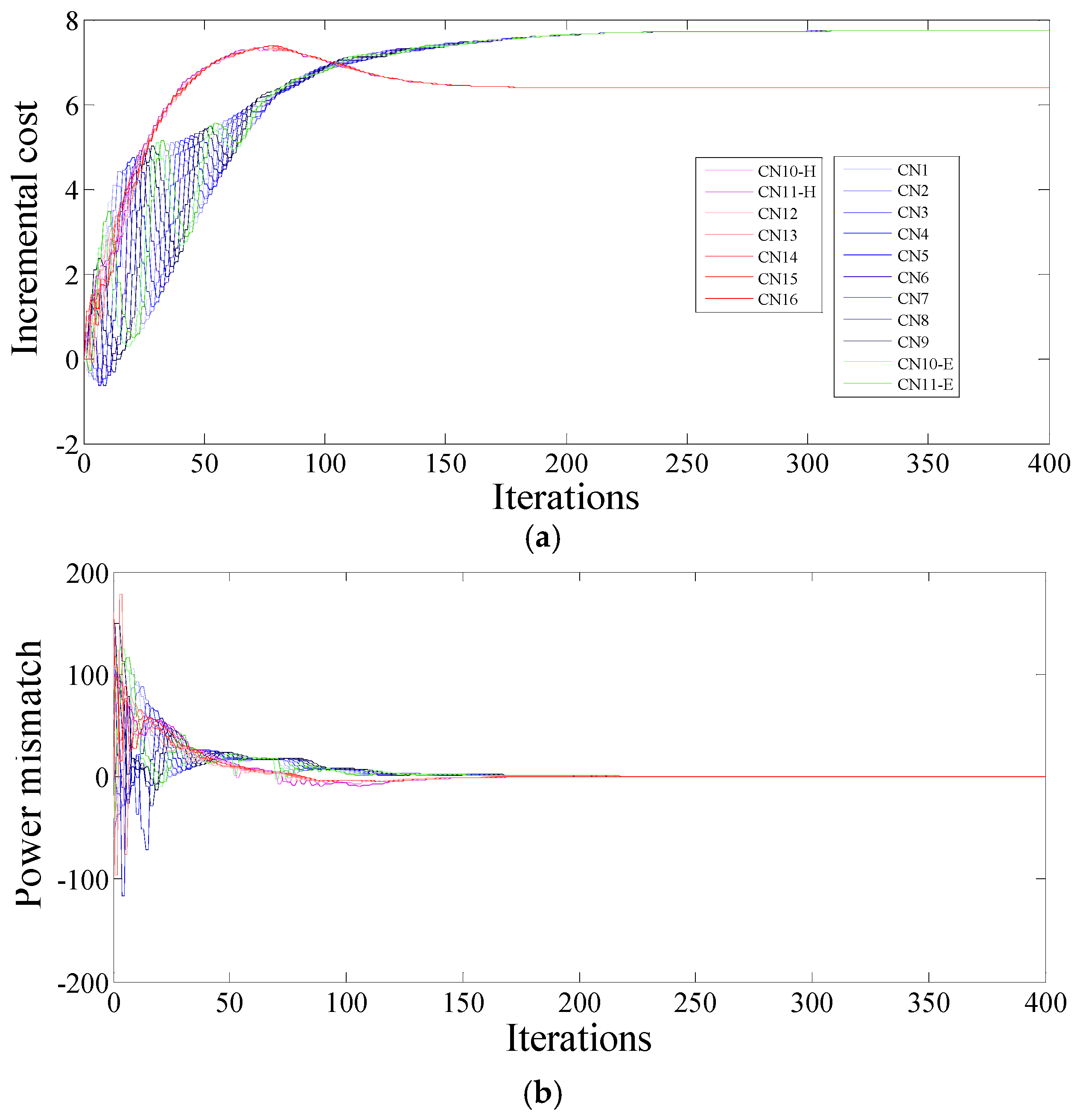
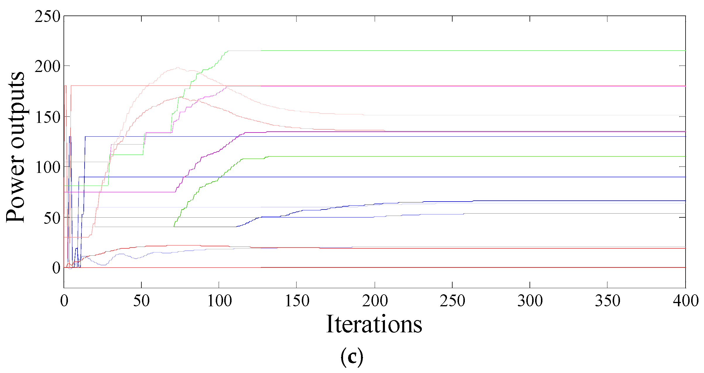
4.1. Case Study 1: Comparison with Centralized Method

In this case study, the focus is on comparing the optimal values between the proposed method and the Lagrangian relaxation method [4]. The initial values can be obtained by Equation (13). The total electrical load demand is 750 (p.u.) with five electrical loads of 150 (p.u.) and the total heat load demand is 800 (p.u.) with five heat loads of 160 (p.u.). Then, the proposed method is used to calculate the optimal solutions. The estimated electrical and heat power incremental cost, mismatch and outputs are shown in Figure 5. It can be seen that all of the electrical and heat power mismatch converge to zeros, which means the supply–demand balance are satisfied. After about 250 iterations, all of the electrical power incremental cost converge to a common value and all of the heat power incremental cost converge to another common value, meanwhile all agents are running in their feasible operating regions and the electrical and heat power outputs are listed in Table 2. In order to further verify the effectiveness of the proposed method, the Lagrangian relaxation method is used to solve this problem in a centralized fashion. The calculation results are also listed in Table 2. It can be seen that the solutions of the two methods are very close, which means the proposed method can also model the optimal values with distributed fashion.

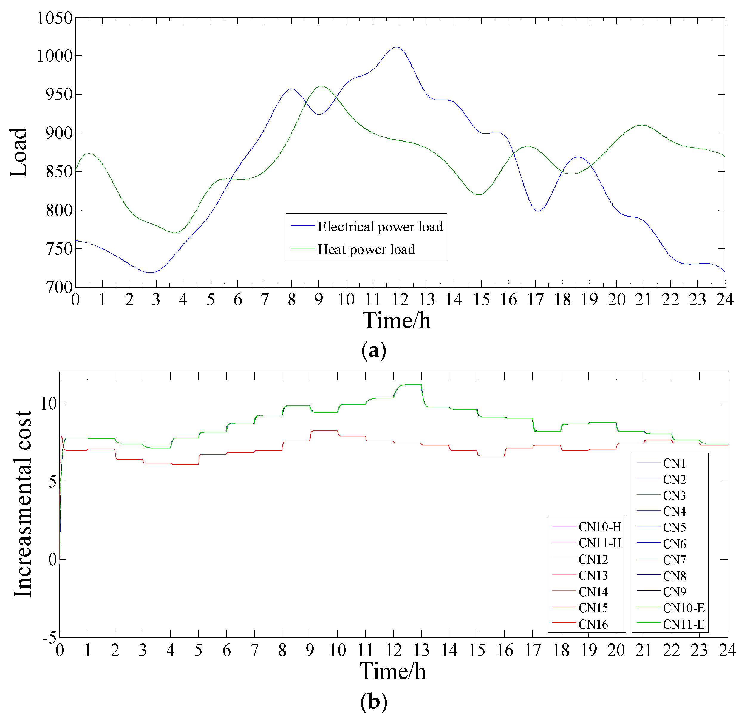
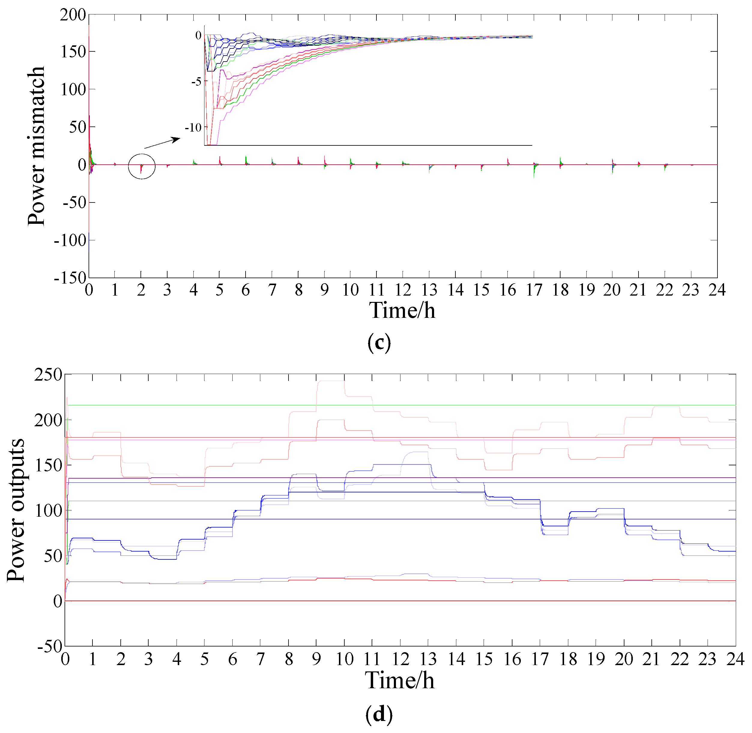
4.2. Case Study 2: Time-Varying Demand

In this case study, the focus is on the performance of the proposed method under time-varying loading conditions. The variable load demands of one day, shown in Figure 6a, are taken into consideration. The scheduling cycle is set to one hour. The initial values can be obtained by Equation (13). Then, the proposed method is used to calculate the optimal solution. From the results shown in Figure 6b–d, it can be observed that the system can automatically converge to new solutions at each scheduling cycle. Both the estimated electrical and heat power incremental cost are modified following the new demand, the estimated electrical and heat power mismatches also converge to zeros meeting the supply–demand balance, and all the electrical and heat power outputs are within their corresponding feasible range. Therefore, this case study verifies that the proposed method can automatically adjust to meet the time-varying loading conditions.

4.3. Case Study 3: Plug and Play Test

In this study case, the focus is on the plug and play adaptability, which is one of the most important advantages of the future CHP system. The initial conditions of are the same as in case 1. The electrical and heat load demands maintain unchanged during the simulation. At time step t = 400 , CGA2 is removed from the test system. It is not very difficult to verify the remaining subgraphs G E C and G H C are also strongly connected. The electrical (heat) loads supplied by CG2 are sent fifty-fifty to its out-neighbors in G E C ( G H C ). From the results in Figure 7, both the electrical and heat incremental cost increase and converge to their new optimal values, meanwhile the electrical and heat power mismatch go to zeros. Of course, the remaining agents have to supply more electrical and heat power to compensate for the electrical and heat power previously supplied by the disconnected CGA2. Moreover, at time step t = 800 , the CGA2 is plugged again in the test system, and the output of CGA2 is set to x 11 p q ( 800 ) = 44 (p.u.), x 11 q p ( 800 ) = 75 (p.u.), y 11 p q ( 800 ) = 44 (p.u.), y 11 q p ( 800 ) = 75 (p.u.), λ 11 p q ( 800 ) = λ 11 q p ( 800 ) = 0 . Then, the system again converges to the new solutions responding to the new topological change. In order to accommodate CGA2, the other agents have to reduce or not change (if the ones have been running on the upper bounders) their electrical and heat power outputs, while CGA2 increases its corresponding outputs. Thus, the electrical and heat incremental cost drop due to the lower average electrical and heat power outputs. In addition, the finally stable values are listed in Table 2. It can be seen that they are very close to the solution prior to disconnection. Therefore, this case study can verify the proposed method performs good plug and play capability.

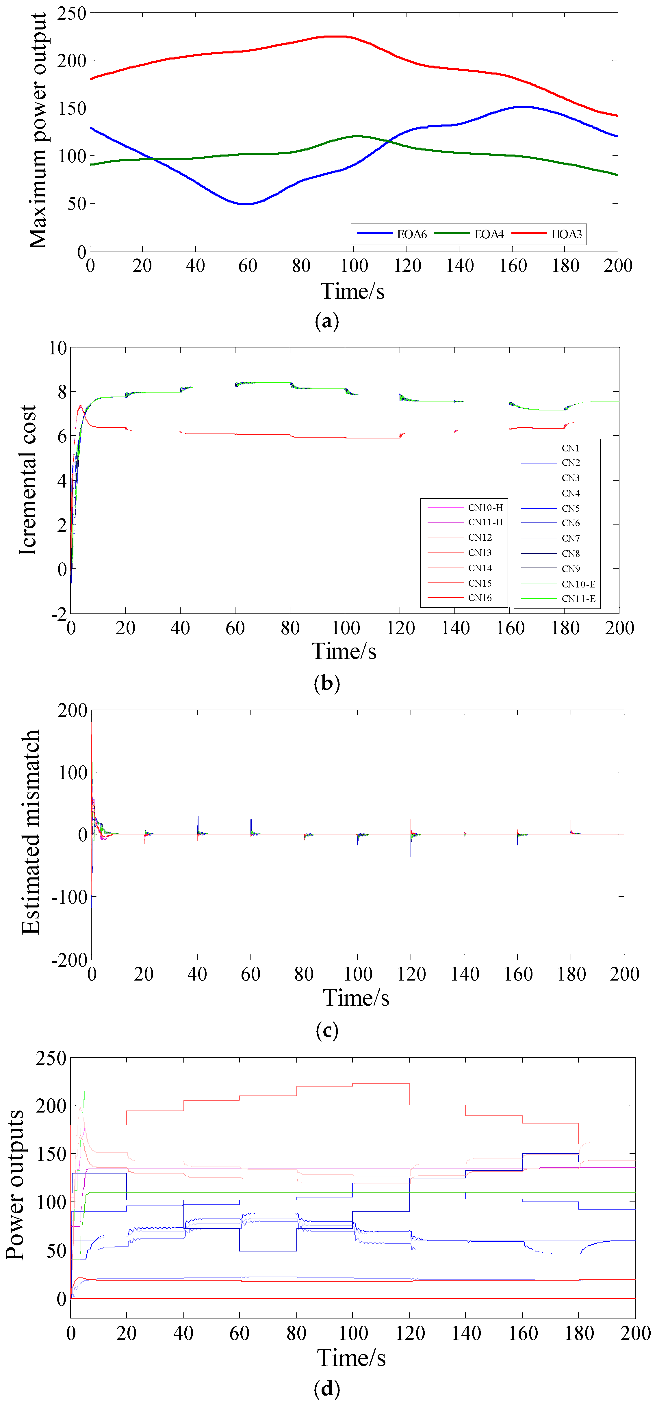
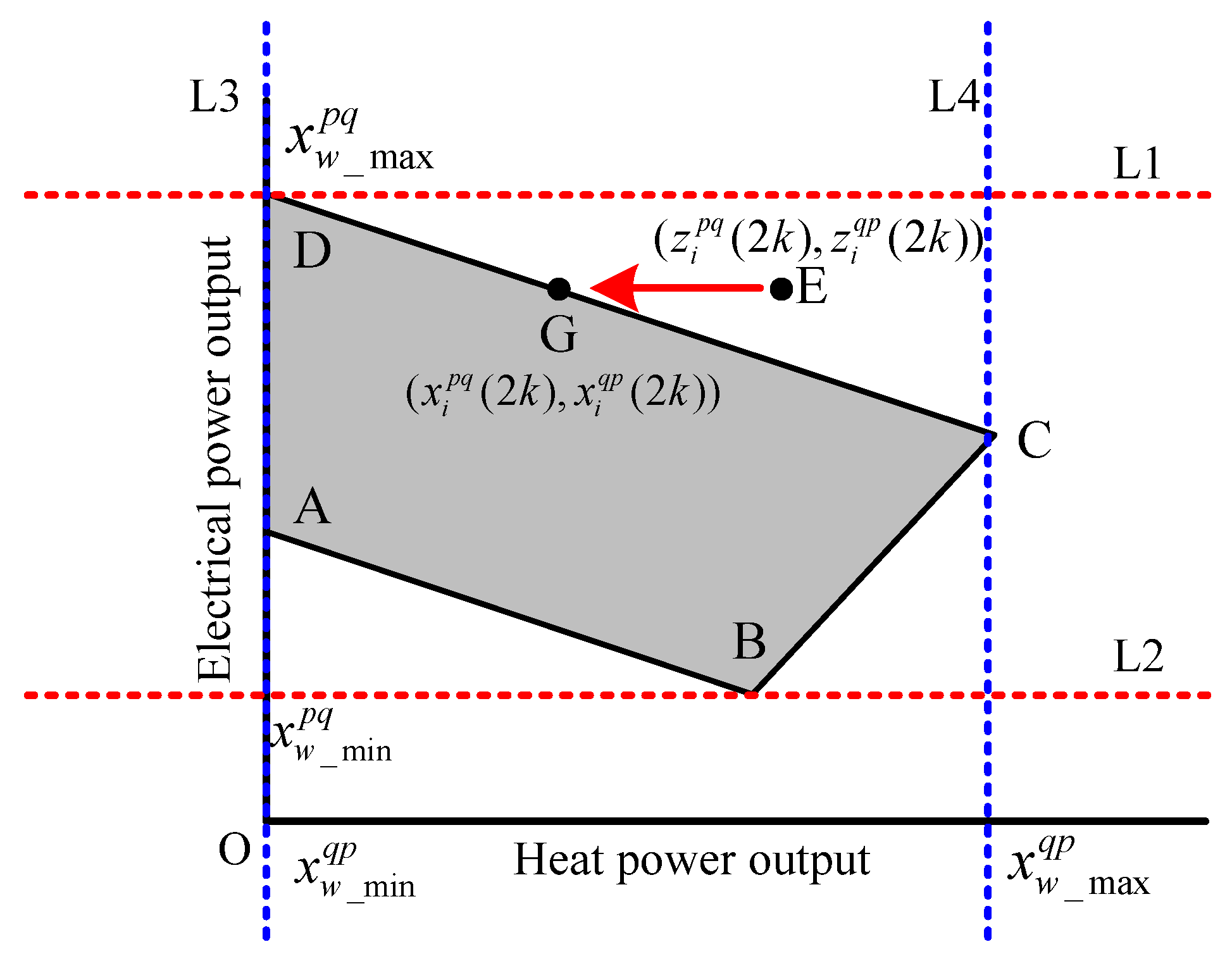
4.4. Case Study 4: Maximum-Power-Output-Varying Condition

In this study case, the focus is on testing the performance of the proposed method when the maximum power output points of RGs and RHDs are changed. In this paper, we let EOA4, EOA6 and HOA3 represent a photovoltaic, a wind generator and a solar water heater, respectively. Their maximum power output profiles are shown in Figure 8a. In this case, the scheduling cycle is set to 20 s, i.e., EOA4, EOA6 and HOA3 measure and reset their corresponding maximum power output point every 20 s. The initial values can be obtained by Equation (13). Then, the proposed method is used to find the optimal operating point during each scheduling cycle. In Figure 8b, it can be observed that, within each scheduling cycle, all of the electrical power incremental costs converge to a common value and all of the heat power incremental costs converge to another common value. That implies the optimization objective is achieved. It is worth noting that the electrical (or heat) incremental cost decreases as the total electrical (or heat) power outputs of EOA4 and EOA6 (or HOA3) increasing. That is because EOA4, EOA6 and HOA3 are renewable energy resources, which have lower cost compared with fuel energy resources. Moreover, Figure 8c shows that both the estimated electrical and heat power mismatches can also converge to zeros within each scheduling cycle, which indicates that the total electrical and heat supply–demand balance constraints are satisfied. In addition, the electrical and heat power outputs are shown in Figure 8d. It can be seen that, within each scheduling cycle, each agent can find its corresponding operating point, which is limited in its feasible operating region. Based on the discussion above, it can be concluded that, by using the proposed method, the system can respond automatically to converge to new solution as the changes of the maximum power outputs of EOA4, EOA6 and HOA3. Therefore, this case study clearly shows that the proposed method can automatically adjust to meet the maximum-power-output-varying condition.

5. Conclusions

A distributed solution for the CHPEDP, taking into consideration multiple-energy-carriers, has been presented. Various kinds of energy conversion devices have been modeled and studied in the problem formulation. The proposed method reaches consensus on the electrical and heat incremental cost, respectively, using corresponding feedback terms that ensure the two supply–demand balance constraints. Because the relationship between the electrical and heat power are coupled, the concept of alternating iterative method has been presented and used to solve the electrical–heating problem, resulting in better solutions. In addition, several simulations have been presented to demonstrate the effect of the proposed method.

Acknowledgments

This work was supported by the National Natural Science Foundation of China Key Program (61573094), and the National Natural Science Foundation of China (61433004, 61603085).

Author Contributions

Yu-Shuai Li conceived the idea for the manuscript and wrote the manuscript with input from Hua-Guang Zhang, Bo-Nan Huang and Fei Teng.

Conflicts of Interest

The authors declare no conflict of interest.

Nomenclature

CHPCombined heat and power
EDPEconomic dispatch problem
DGsDistributed generators
RGsRenewable generators
FGsConventional fuel generators
DHDsDistributed heating devices
RHDsRenewable heating devices
FHDsConventional fuel heating devices
DESDsDistributed energy storage devices
EESDsElectrical energy storage devices
HESDsHeat energy storage devices
RCHPsRenewable combined heat and power
FCHPsFuel combined heat and power
EOAsElectricity-only agents
CGAsCo-generation agents
HOAsHeat-only agents
i , j Agent indices
n 1 , n 2 , n 3 The number of EOAs, CGAs and HOAs, respectively
t , η Iteration-step and step-size
a i , b i , α i , β i , γ i and ξ i Cost coefficients
x i p q , x i q p Electrical power and heat power outputs of CGA i
x i p Electrical power output of EOA i
x i q Heat power output of HOA i
x min p q ( x q p ) , x max p q ( x q p ) Upper and lower bound functions of x p q
x min q p ( x p q ) , x max q p ( x p q ) Upper and lower bound functions of x p q
x i _ min p , x i _ max p Lower and upper bounds of x i p
d m , e m , f m Coefficients of the set of linear constraints of CGA
x i _ min q , x i _ max q Lower and upper bounds of x i q
x w _ min p q , x w _ max p q Whole minimum and maximum values for all of x p q
x w _ min q p , x w _ max q p Whole minimum and maximum values for all of x p q
x i _ M P P T _ max p , x i _ M P P T _ max q Maximum peak power tracking point of RG and RHD
x i _ w _ max p , x i _ w _ max q System maximum capacity of RG and RHDs
x i _ B p q , x i _ B q p Values of point B
D P , D Q Total electrical power and heat power demands
L i _ E , L i _ H Local electrical and heat load demands associated with agent i
λ p , λ p Lagrange multipliers for the equality constraints
μ i _ min , μ i _ max Lagrange multipliers for inequality constraints.
λ p * , λ q * The optimal electrical and heat incremental costs
χ i One of state variable of agent i
χ The column stack vector of χ i
ω T Normalized left eigenvector of R associated to the eigenvalue 1
λ i θ ( t ) , λ i ϑ ( t ) Estimated electrical and heat incremental costs
z i θ ( t ) , z i ϑ ( t ) Estimated electrical and heat power outputs before considering inequality constraints
x i θ ( t ) , x i ϑ ( t ) Estimated electrical and heat power outputs after considering inequality constraints
y i θ ( t ) , y i ϑ ( t ) Estimated electrical and heat power mismatches

Appendix A

Firstly, we do not take the inequality constraints into consideration. That means x = [ x i p , x i p q , x i q p , x i q ] is always equal to z = [ z i p , z i p q , z i q p , z i q ] . Since, in the odd-numbered iteration, Θ ( 2 k 1 ) = Θ ( 2 k 2 ) is satisfied, then Equation (11) can be re-written as the following matrix form.
λ ϑ ( 2 k ) = R ¯ λ ϑ ( 2 k 2 ) + η y ϑ ( 2 k 2 ) Z ϑ ( 2 k ) = E λ ϑ ( 2 k ) + F Y ϑ ( 2 k ) = S ¯ Y ϑ ( 2 k 2 ) Z ϑ ( 2 k ) + Z ϑ ( 2 k 2 )
where λ ϑ = [ λ q p T , λ q T ] T , Z ϑ = [ Z q p T , Z q T ] T and Y ϑ = [ Y q p T , Y q T ] T . Therein, λ q p , λ q , Z q p , Z q , Y q p and Y q are the column vectors of λ i q p , λ i q , z i q p , z i q , y i q p and y i q , respectively. E = d i a g ( [ 1 / 2 α n 1 + 1 , , 1 / 2 α n 1 + n 2 + n 3 ] ) and F = d i a g ( [ ψ n 1 + 1 , , ψ n 1 + n 2 , β n 1 + n 2 + 1 / 2 α n 1 + n 2 + 1 ,···, β n 1 + n 2 + n 3 / 2 α n 1 + n 2 + n 3 ] ) . Therein, ψ i = ( β i + ξ i z i p q ( 2 k 1 ) ) / 2 α i .
Equation (A1) can be further simplified as
[ λ ϑ ( 2 k ) Y ϑ ( 2 k ) ] = ( Γ + η Ω ) [ λ ϑ ( 2 k 2 ) Y ϑ ( 2 k 2 ) ]
where Γ = [ R ¯ 0 E ( I R ¯ ) S ¯ ] and Ω = [ 0 I 0 E ] .
Note that the eigenvalues of Γ are the unions of the eigenvalues of R ¯ and S ¯ . According to Lemma 4 of [26], it is not difficult to verify that both R ¯ and S ¯ have a single eigenvalue with maximum modulus of 1, and there exist ω ¯ T and υ ¯ satisfying ω ¯ T S ¯ = ω ¯ T with ω ¯ T 1 = 1 and R ¯ υ ¯ = υ ¯ with 1 T υ ¯ = 1 . In addition, the other eigenvalues are located strictly inside a unit disk. Thus, Γ has two eigenvalue with modulus of 1, denoted as = ƛ = 1 .
Then, the eigenvalue perturbation method is further used to study the eigenvalue changing of Γ perturbed by Ω . We construct the following two matrices
W = [ 1 T E 1 T ω ¯ T 0 T ] , V = [ 0 1 υ ¯ ρ υ ¯ ]
where ρ = i = n 1 + 1 n 1 + n 2 + n 3 1 / 2 α i . In this way, we can get W V = I .
Furthermore, the change of and ƛ can be quantified by the eigenvalues of Μ as follows
Μ = W Ω V = [ 0 0 ω ¯ T υ ¯ ρ ω ¯ T υ ¯ ]
It is easy to obtain that d / d η = 0 and d ƛ / d η = ρ ω ¯ T υ ¯ < 0 are the two eigenvalues of Μ . That implies does not change; meanwhile, ƛ becomes smaller. Thus, there exist an upper bound η ˜ for η , such that | ƛ | < 1 if 0 < η < η ˜ . Therefore, except for = 1 , the others are located strictly inside a unit disk. More importantly, it can be verified that [ 1 T , 0 T ] T is the eigenvector of Γ + η Ω . That implies y i q p and y i q converge to zero; meanwhile, λ i q p and λ i q converge to a common value. Thus, the optimal conditions are satisfied, In addition, when the inequality constraints are taken into consideration, the projection operators Equation (11c) does not affect the convergence which has been verify in [20,24]. Then, we can conclude that λ i q λ q * , λ i q p λ q * , x i q x i q * and x i q p x i q p * , as 2 k .
By using the similar process of the proof above, we can obtain that y i p and y i p q converge to zero; meanwhile, λ i p and λ i p q converge to another common value. Then, we can get λ i p λ p * , λ i p q λ p * , x i p x i p * and x i p q x i p q * as 2 k + 1 .
The proof is over.

References

  1. Conti, S.; Faraci, G.; Corte, A.L.; Nicolosi, R.; Rizzo, S.A.; Schembra, G. Effect of islanding and telecontrolled switches on distribution system reliability considering load and green-energy fluctuations. Appl. Sci. 2016, 6, 1–26. [Google Scholar] [CrossRef]
  2. Peng, C.; Lei, S.; Hou, Y.; Wu, F. Uncertainty management in power system operation. CSEE J. Power Energy Syst. 2015, 1, 28–35. [Google Scholar] [CrossRef]
  3. Huang, C.; Yue, D.; Xie, J.; Li, Y.; Wang, K. Economic dispatch of power systems with virtual power plant based interval optimization method. CSEE J. Power Energy Syst. 2016, 1, 74–80. [Google Scholar] [CrossRef]
  4. Guo, T.; Henwood, M.I.; van Ooijen, M. An algorithm for combined heat and power economic dispatch. IEEE Trans. Power Syst. 1996, 11, 1778–1784. [Google Scholar] [CrossRef]
  5. Sashirekha, A.; Pasupuleti, J.; Moin, N.H.; Tan, C.S. Combined heat and power (CHP) economic dispatch solved using Lagrangian relaxation with surrogate subgradient multiplier updates. Int. J. Electr. Power Energy Syst. 2013, 44, 421–430. [Google Scholar] [CrossRef]
  6. Niknam, T.; Azizipanah-Abarghooee, R.; Roosta, A.; Babak, A. A new multi-objective reserve constrained combined heat and power dynamic economic emission dispatch. Energy 2012, 42, 530–545. [Google Scholar] [CrossRef]
  7. Liu, Z.; Chen, C.; Yuan, J. Hybrid energy scheduling in a renewable micro grid. Appl. Sci. 2015, 5, 516–531. [Google Scholar] [CrossRef]
  8. Huang, X.C.; Yang, Y.; Taylor, G.A. Service restoration of distribution systems under distributed generation scenarios. CSEE J. Power Energy Syst. 2016, 2, 43–50. [Google Scholar]
  9. Samimi, A.; Kazemi, A. Coordinated volt/var control in distribution systems with distributed generations based on joint active and reactive powers dispatch. Appl. Sci. 2016, 6, 1–17. [Google Scholar] [CrossRef]
  10. Zhang, H.; Feng, T.; Yang, G.H.; Liang, H. Distributed cooperative optimal control for multiagent systems on directed graphs: An inverse optimal method. IEEE Trans. Cybern. 2015, 45, 1315–1326. [Google Scholar] [CrossRef] [PubMed]
  11. Sun, Q.; Zhang, Y.; He, H.; Ma, D.; Zhang, H. A Novel Energy Function-Based Stability Evaluation and Nonlinear Control Method for Energy Internet. IEEE Trans. Smart Grid 2016. [Google Scholar] [CrossRef]
  12. Zhang, H.; Qing, C.; Luo, Y. Neural-network-based constrained optimal control scheme for discrete-time switched nonlinear system using dual heuristic programming. IEEE Trans. Autom. Sci. Eng. 2014, 11, 839–849. [Google Scholar] [CrossRef]
  13. Samimi, A.; Kazemi, A. A new method to optimal allocation of reactive power ancillary service in distribution systems in the presence of distributed energy resources. Appl. Sci. 2015, 5, 1284–1309. [Google Scholar] [CrossRef]
  14. Zhang, H.; Kim, S.; Zhou, J. Distributed adaptive virtual impedance control for accurate reactive power sharing based on consensus control in microgrids. IEEE Trans. Smart Grid 2016. [Google Scholar] [CrossRef]
  15. Shi, W.; Xie, X.; Chu, C.C.; Gadh, R. Distributed optimal energy management in microgrids. IEEE Trans. Smart Grid 2015, 6, 1137–1146. [Google Scholar] [CrossRef]
  16. Zhang, H.; Feng, T.; Liang, H.; Luo, Y. LQR-Based optimal distributed cooperative design for linear discrete-time multiagent systems. IEEE Trans. Neural Netw. Learn. Syst. 2016. [Google Scholar] [CrossRef] [PubMed]
  17. Yang, S.; Tan, S.; Xu, J.X. Consensus based method for economic dispatch problem in a smart grid. IEEE Trans. Power Syst. 2013, 28, 4416–4426. [Google Scholar] [CrossRef]
  18. Loia, V.; Vaccaro, A. Decentralized economic dispatch in smart grids by self-organizing dynamic agents. IEEE Trans. Syst. Man Cybern. Syst. 2014, 44, 397–408. [Google Scholar] [CrossRef]
  19. Binetti, G.; Davoudi, A.; Lewis, F.L.; Naso, D.; Turchiano, B. Distributed consensus-based economic dispatch with transmission losses. IEEE Trans. Power Syst. 2014, 29, 1711–1720. [Google Scholar] [CrossRef]
  20. Rahbari-Asr, N.; Ojha, U.; Zhang, Z.; Chow, M.-Y. Incremental welfare consensus method for cooperative distributed generation/demand response in smart grid. IEEE Trans. Smart Grid 2014, 5, 2836–2845. [Google Scholar] [CrossRef]
  21. Xu, Y.; Li, Z. Distributed optimal resource management based on consensus method in a microgrid. IEEE Trans. Ind. Electron. 2015, 62, 2584–2592. [Google Scholar] [CrossRef]
  22. Xu, Y.; Zhang, W.; Liu, W. Distributed dynamic programming-based method for economic dispatch in smart grids. IEEE Trans. Ind. Inf. 2015, 11, 166–175. [Google Scholar] [CrossRef]
  23. Binetti, G.; Davoudi, A.; Naso, D.; Turchiano, B.; Lewis, F.L. A distributed auction-based method for the non-convex economic dispatch problem. IEEE Trans. Ind. Inf. 2014, 10, 1124–1132. [Google Scholar] [CrossRef]
  24. Zhang, W.; Xu, Y.; Liu, W.; Zhang, C.; Yu, H. Distributed Online optimal energy management for smart grids. IEEE Trans. Ind. Inf. 2015, 11, 717–727. [Google Scholar] [CrossRef]
  25. Nutkani, I.U.; Loh, P.C.; Wang, P.; Blaabjerg, F. Cost-prioritized droop schemes for autonomous microgrids. IEEE Trans. Power Electron. 2015, 30, 1021–1025. [Google Scholar] [CrossRef]
  26. Olfati-Saber, R.; Fax, A.; Murray, R.M. Consensus and cooperation in networked multi-agent systems. Proc. IEEE 2007, 95, 215–233. [Google Scholar] [CrossRef]
Figure 1. A structure of combined heat and power (CHP) system.
Applsci 06 00308 g001
Figure 2. Feasible operating region of co-generation agents (CGA).
Applsci 06 00308 g002
Figure 3. The 16-bus test system.
Applsci 06 00308 g003
Figure 4. Feasible operating region of CGA1 and CGA2.
Applsci 06 00308 g004
Figure 5. Case study 1, comparison with centralized scheme: (a) estimated electrical and heat incremental cost; (b) estimated electrical and heat power mismatch; and (c) electrical and heat power outputs.
Applsci 06 00308 g005aApplsci 06 00308 g005b
Figure 6. Case study 2, time-varying demand: (a) electrical and heat power load demands; (b) estimated electrical and heat incremental cost; (c) estimated electrical and heat power mismatch; and (d) electrical and heat power outputs.
Applsci 06 00308 g006aApplsci 06 00308 g006b
Figure 7. Case study 3, plug and play test: (a) estimated electrical and heat incremental cost; (b) estimated electrical and heat power mismatch; and (c) electrical and heat power outputs.
Applsci 06 00308 g007
Figure 8. Case study 4, maximum power output varying: (a) maximum power output; (b) estimated electrical and heat incremental cost; (c) estimated electrical and heat power mismatch; and (d) electrical and heat power outputs.
Applsci 06 00308 g008
Table 1. Parameters of the 16-bus system.
Agent a b α β ε MinMax
EOA10.01745.5---60180
EOA20.1880----−7575
EOA30.01246.4---50150
EOA40.00040.106---0140
EOA50.01465.8---40120
EOA60.00090.02---0180
CGA10.00692.90.00600.840.0062--
CGA20.00875.00.00540.120.0022--
HOA1--0.01023.3-40500
HOA2--0.01462.42-30300
HOA3--0.00010.084-0250
HOA4--0.1660--−200200
Table 2. Comparison for the 16-bus system.
AgentCase Study 1: Proposed MethodCase Study 1: Centralized MethodCase Study 2: Proposed Method
EOA164.135564.198764.1676
EOA220.563620.569520.5666
EOA353.707853.795053.7544
EOA490.000090.000090.0000
EOA566.165066.236866.2062
EOA6130.0000130.0000130.0000
CGA1-E215.1412215.0000215.0399
CGA2-E110.2749110.2000110.2529
CGA1-H179.2058180.0000179.7754
CGA2-H134.9488135.6000135.1400
HOA1150.9958150.1772150.5662
HOA2135.6291135.0553135.32714
HOA3180.0000180.0000180.0000
HOA419.218019.167519.1914
Total cost5811.35806.95809.3

