Auralization of Accelerating Passenger Cars Using Spectral Modeling Synthesis

Abstract

While the technique of auralization has been in use for quite some time in architectural acoustics, the application to environmental noise has been discovered only recently. With road traffic noise being the dominant noise source in most countries, particular interest lies in the synthesis of realistic pass-by sounds. This article describes an auralizator for pass-bys of accelerating passenger cars. The key element is a synthesizer that simulates the acoustical emission of different vehicles, driving on different surfaces, under different operating conditions. Audio signals for the emitted tire noise, as well as the propulsion noise are generated using spectral modeling synthesis, which gives complete control of the signal characteristics. The sound of propulsion is synthesized as a function of instantaneous engine speed, engine load and emission angle, whereas the sound of tires is created in dependence of vehicle speed and emission angle. The sound propagation is simulated by applying a series of time-variant digital filters. To obtain the corresponding steering parameters of the synthesizer, controlled experiments were carried out. The tire noise parameters were determined from coast-by measurements of passenger cars with idling engines. To obtain the propulsion noise parameters, measurements at different engine speeds, engine loads and emission angles were performed using a chassis dynamometer. The article shows how, from the measured data, the synthesizer parameters are calculated using audio signal processing.

1. Introduction

Noise caused by traffic is a relevant health factor in urban environments, along major transport routes and in the vicinity of airports. Noise, in contrast to sound, can principally not be measured, but has to be assessed. For the most relevant noise sources, objective quantities have been derived that correlate with the annoyance as reported by people. However, these correlations are usually weak. One reason for this is the fact that the describing quantities used so far represent the acoustic situation only in a very simplified manner. A method to further investigate the signal properties relevant to noise is to conduct listening experiments where different stimuli are presented to test persons. Relying on audio recordings allows for little variation of different signal aspects only. A more versatile method with a much higher degree of freedom, as well as full control of the influencing signal parameters is to synthesize the stimuli and, thus, to auralize an acoustical environment.

Auralization has been in use for quite some time in architectural acoustics, namely in the fields of room and building acoustics [1,2,3], but it has only recently been discovered for environmental acoustical applications. Today, most auralizations are generated based on computer models and digital signal processing. However, between applications, the individual simulation steps may vary significantly. In room and building acoustical auralizations, it is common to utilize (anechoic) recordings as the source material, whereas in environmental acoustics, it is often required to artificially synthesize the source signals [4,5,6,7,8]. Furthermore, the sound propagation simulation substantially differs. In room acoustical auralizations, the focus lies on the simulation of many room reflections, in particular specular vs. diffuse reflections, and diffraction [2,3]. In building acoustical auralizations, sound transmission through structures is simulated using sound insulation prediction models [2]. For environmental acoustical auralizations, however, particular emphasis is placed on a detailed simulation of direct sound and ground reflection. Leastwise, in terms of sound reproduction, the same techniques are applicable.

Early attempts in auralizations for environmental noise applications have been made by a group at NASA Langley Research Center, where aircraft flyovers have been binaurally rendered based on monaural recordings [9]. In the same period, a synthesis model for the traction noise of electric rail-bound vehicles was developed at the RWTH Aachen University and used to study sound quality [4]. Newer auralization models also try to synthesize the sounds of aircraft [7,8,10]. One of these models has already been combined with 3D visualizations to make aircraft noise both heard and seen in immersive virtual reality environments [8]. In the recently-completed Swiss project “VisAsim” [11,12], outdoor auralizations of wind farms were linked to synchronous GIS-based 3D visualizations. Within the Swedish project “LISTEN” [13,14] and the European project “HOSANNA” [5,15], tools for the auralization of road traffic noise were developed. The main motivation is to provide more intuitive information about traffic noise scenarios for city planners, noise consultants and decision makers. There is common agreement in the point that information about noise in the form of dB values is difficult to communicate to the public [16]. On the other hand, there is growing interest in the perceptual aspects of noise abatement measures. While in the past, the quality of noise mitigation measures was understood as the A-weighted sound pressure level reduction, the focus shifts to perceptual efficiency [17]. In this respect the optimal measure is not necessarily the one with the highest dB(A) drop, but the one with the highest annoyance reduction. The idea of describing and subsequently improving the acoustical environment with respect to human perception corresponds to the soundscape concept.

Generally, the auralization process consists of three modules [2]. The first module provides the signal emitted at the source. In its simplest form, this emission module makes use of suitable audio recordings. Obviously, the disadvantage of this strategy is its inflexibility, the limitations with respect to possible emission signal variations and the fundamental difficulty to obtain recordings that are not contaminated by unwanted sound. In addition, due to the Doppler effect, recordings of moving sources can be used for the auralization of situations with similar geometries only. It is therefore promising to use a digital emission synthesizer that is capable of generating the audio signal as radiated by the source. In [5], a granular synthesis using an enhanced pitch-synchronous overlap-and-add (PSOLA) method is presented for engine noise. This method features low computational costs and is therefore well suited for real-time applications. It is however limited in terms of flexibility, as it does not allow for inter- and extrapolations between measured signals. This limitation can be overcome by the synthesizer presented in this article, at the expense of computational costs.

The second module needed in the auralization process is a filter that simulates the sound propagation effects of the wave traveling from the source to the receiver. These effects involve geometrical spreading, propagation delay and atmospheric absorption. In outdoor situations, along with the direct sound path, also reflections occur, particularly ground reflections, leading to the ground effect. When either the source or the receiver moves, additionally, the Doppler effect arises. However, also, due to the time-varying propagation situation, all of the other effects change over time, which means that the propagation filter becomes time variant [18].

The third module is a reproduction system, which renders the received signals to headphones or a multi-channel loudspeaker system. In this process, for every received signal, its corresponding emission angle with respect to the observer is required. For the rendering, a variety of different methods exists [19]. Further, it has to be assured that the reproduction system has a linear frequency response and that it is correctly calibrated.

In the ongoing research project “TAURA”, a traffic noise auralizator is developed that covers road traffic and railway noise. It will form the basis for future experiments to refine the characterization of noise. The key element is a synthesizer that simulates the acoustical emission of a great many different vehicles, operating on a wide variety of surfaces and under different operating conditions. In the TAURA model, road traffic noise is created by the superposition of individual vehicle pass-by sounds. The objective of this article is to describe how these single pass-by sounds can be generated in the case of passenger cars.

This paper extends the work presented in [20] and is structured in two main parts: In Section 2, the auralization model of accelerating passenger cars is developed step by step and presented. Thereby, an emission synthesizer, which is based on spectral modeling synthesis, and propagation filtering algorithms are elucidated. Section 3 shows how the model parameters can be estimated based on controlled measurements. On that account, a series of signal analysis steps to obtain the steering parameters of the synthesizer is proposed. The article ends with conclusions in Section 4.

2. Model Development

2.1. Overview

This section presents an overview of the model to auralize accelerating passenger cars. Further, the key assumptions and motivations used for the model development are presented. In the model, each car is represented by two moving point sources. The geometrical situation is depicted in Figure 1, in which the distance of the straight driving lane to the receiver is D, the emission angle $\phi$, the angle of inclination α and the point source positions S1 and S2, respectively. Describing the kinematics of the vehicle, its speed $v\left(t\right)$ in km/h as a function of time t (at the source) is used throughout this paper. In correspondence with the Harmonoise model [21], the point sources are vertically stacked and located at heights of 0.01 and 0.3 m above ground. By not attributing separate point sources to each vehicle axle, we limit the applicability of the model to situations with source–receiver distances clearly larger than the axial distance, while in return, saving computational costs.

Figure 1. Sketch of the geometrical situation showing the two source positions S1 and S2, the inclination angle of the road α, the distance D, the instantaneous vehicle speed v, emission angle $\phi$, immmission angle θ and source–receiver distance r.

Figure 1. Sketch of the geometrical situation showing the two source positions S1 and S2, the inclination angle of the road α, the distance D, the instantaneous vehicle speed v, emission angle $\phi$, immmission angle θ and source–receiver distance r.

Road traffic noise is mainly composed of propulsion noise and tire noise [18,21,22,23]. Both contributions differ in their relevance for the total noise, depending on the vehicle, its operating conditions and the pavement type. This motivates that in the presented model, the contributions of propulsion noise and tire noise are simulated individually.

In accordance with Vorländer’s definition of the “principle of auralization” [2], the presented model to auralize accelerating passenger cars comprises a separate emission, a propagation and a reproduction module. The emission module is described in Section 2.2, the propagation module in Section 2.3 and the reproduction module in Section 2.4. Figure 2 shows the block diagram of the model. The input variables describe the vehicle, driver, road surface, geometry, ground type and the weather; the input variables marked by * are time dependent.

Figure 2. Simulation flowchart of the auralization of accelerating passenger cars. The input variables marked by a * are time dependent.

Figure 2. Simulation flowchart of the auralization of accelerating passenger cars. The input variables marked by a * are time dependent.

The emission module describes the emitted sound of an individual passenger car pass-by, i.e., its outside sound. In Figure 2, the emission module is edged by a gray dashed line. It contains several simulation blocks creating two separate signal paths. The upper path (red box) represents the propulsion noise and the lower path (blue box) the tire noise simulation. Key elements are two sound synthesizers that artificially generate audible emission signals for propulsion and tire noise, respectively. The synthesizer parameters can be obtained from controlled measurements, as elucidated in Section 3. Section 2.2 describes how the synthesized emission signals are attributed to the two point sources. As a proper interface to the propagation module, the point source signals are defined at a virtual reference distance of $r_0=1$ m [6]. They feature time-varying sound characteristics and already include source directivity.

For both moving source positions, S1 and S2, the sound propagation to the (static) receiver position is simulated in the propagation module. To generate the receiver signals, both corresponding source signals, $s_1$ and $s_2$, are filtered by a series of time-varying digital filters, as described in Section 2.3. These filters depend on the instantaneous propagation geometry, the ground type and the weather conditions (cf. Figure 2). Finally, in the reproduction module, the receiver signals are summed up and rendered for multi-channel reproduction using the instantaneous immission angle. Section 2.4 exemplifies a possible stereo rendering procedure.

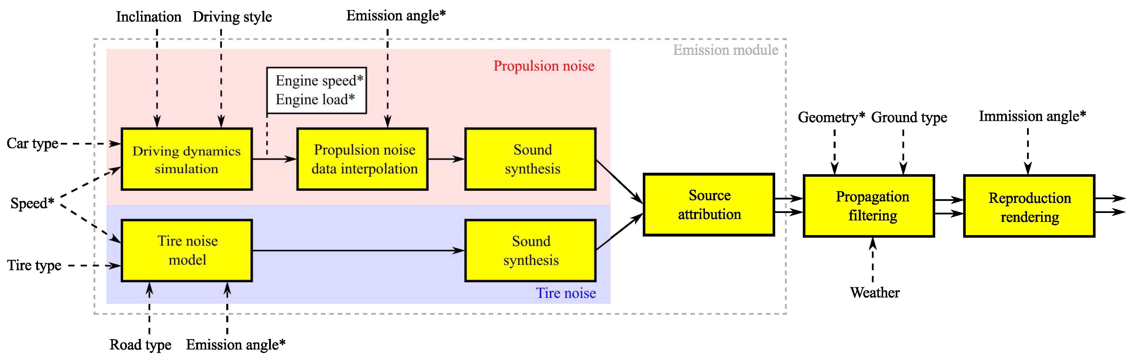
2.2. Emission Module

The emission module describes the emitted sounds of an individual passenger car. Its structure is depicted in Figure 2. As described above, the acoustical emission of the passenger car is assumed to consist of the two contributions: tire noise and propulsion noise. Their corresponding emission signals are denoted as $s_{\mathrm{tire}}$ and $s_{\mathrm{prop}}$, respectively.

Tire noise strongly depends on tire type [22,24], road surface type [18,21,22,25] and vehicle speed [18,21,22,23]. Further, the horn effect mainly determines the horizontal directivity of tire noise [21,23,26]. To model these effects, the tire noise contribution is assumed to depend on the road and tire type, as well as on vehicle speed v and the emission angle $\phi$. Section 2.2.1 shows how the signals $s_{\mathrm{tire}}$ are calculated based on these input parameters.

In current noise prediction models, propulsion noise is commonly calculated as a function of vehicle speed, acceleration and road inclination [18,21,27]. This is due to the fact that these models are developed and used in cases for which the engaged gear is not known. The gear, however, strongly influences the sound of propulsion [23]. For a given speed, acceleration and road inclination, by changing the gear, the engine speed, as well as the engine load change. From an engine’s viewpoint, it is these two parameters that are sufficient to fully describe the engine condition. Section 2.2.2 explains how in the auralization model, engine speed n and engine load Γ are calculated by simulating the driving dynamics of the vehicle. These simulations require information on the vehicle and the driving style, the road inclination α and the vehicle speed $v\left(t\right)$ as a function of time t. Further, propulsion noise features a directivity [23], which is also taken into account in the auralization model. Section 2.2.3 shows how, based on n, Γ and the emission angle $\phi$, the signal $s_{\mathrm{prop}}$ is calculated.

The audible emission signals $s_{\mathrm{tire}}$ and $s_{\mathrm{prop}}$ are generated artificially by two digital sound synthesizers. The synthesizers are based on a combination of additive and subtractive synthesis. In additive synthesis, the signal is constructed by the sum of sinusoids, each having a time-varying amplitude and phase [28,29,30]. On the other hand, subtractive synthesis uses filters to shape a more complex source signal, e.g., a sawtooth wave or white noise [28,29]. The combination of both techniques is known as spectral modeling synthesis [30,31,32]. However, in contrast to the applications presented in [31] and [32], in the presented model, the sounds are not synthesized using the short-time Fourier transform (STFT), but directly in the time domain. The structure of the synthesizer is similar to the one recently published for wind turbine sounds [6].

The signal of propulsion noise, $s_{\mathrm{prop}}$, is fully attributed to the upper point source S2. However, the sound power of the tire noise contribution is attributed to the point sources by 80%/20% [21]. This translates to a ratio of 2:1 of their respective sound pressure signals. The conditions of incoherent signals and energy conservation yield a normalization factor of $1/\sqrt{5}$. Thus, the sound pressure source signals are:

$$\begin{array}{ccc}\hfill s_2\left(t\right)& =& \frac{1}{\sqrt{5}}·s_{\mathrm{tire},2}\left(t\right)+s_{\mathrm{prop}}\left(t\right)\hfill \end{array}$$

(1)

$$\begin{array}{ccc}\hfill s_1\left(t\right)& =& \frac{2}{\sqrt{5}}·s_{\mathrm{tire},1}\left(t\right)\hfill \end{array}$$

(2)

at reference distance $r_0=1$ m for source positions S2 and S1, respectively. Indices 2 and 1 indicate that different, uncorrelated signals for the sound of tires are generated for the two source positions.

2.2.1. Sound of Tires

The emission signal of the sound of tires is assumed to consist of broadband noise only, i.e., discrete tones due to, e.g., tire tread resonances or discrete vibrational tire resonances are not taken into account.

The spectral shaping of the broadband noise components is performed in 1/3 octave bands. For each 1/3 octave band i, white noise is generated and filtered by a digital pink filter. This pre-shaping helps to produce a smoother spectrum of the resulting signal [6]. The output of the pink filter is bandpass filtered by an eighth order Butterworth filter (Class 0 according to the standard IEC 1260:1995 [33]) and normalized to unit signal power to obtain the signal ${\xi }_i\left(t\right)$. For stability reasons, also at low frequencies, the filters are implemented as cascaded second-order sections (SOS).

The sound pressure emission signals of the sound of tires component are thus calculated by [6]:

$$s_{\mathrm{tire}}\left(t\right)=\sum _{i=1}^{N_b}{p}_0{10}^{L_{\mathrm{tire},i}(v\left(t\right),\phi \left(t\right))/20}·{\xi }_i\left(t\right)$$

(3)

with $N_b$ being the number of considered 1/3 octave bands, the reference pressure $p_0$ = 20 μPa and normalized bandpass filtered pink noise signals ${\xi }_i\left(t\right)$. A total of $N_b=29$ bands from 20 Hz to 12.5 kHz are used. For the sound pressure level $L_{\mathrm{tire},i}$ of band i, a common logarithmic speed relationship [22] with additive correction terms is assumed:

$$L_{\mathrm{tire},i}\left(t\right)=A_i+B_i·log\left(\frac{v\left(t\right)}{v_0}\right)+\Delta L_{\mathrm{road},i}\left(v\left(t\right)\right)+\Delta L_{\mathrm{dir},i}\left(\phi \left(t\right)\right)$$

(4)

with reference speed $v_0=70$ km/h, regression parameters $A_i$ and $B_i$, the road surface correction $\Delta L_{\mathrm{road},i}$ and a horizontal directivity $\Delta L_{\mathrm{dir},i}$. For the road surface correction, the Swiss “sonRoad” model [18] offers the parameter ${\Delta }_{\mathrm{BG}}$ for 10 surface types. However, ${\Delta }_{\mathrm{BG}}$ does not depend on frequency or vehicle speed. The recently-published EU directive on establishing common noise assessment methods (CNOSSOS-EU) [27] contains spectral corrections in octave bands in the form of:

$$\Delta L_{\mathrm{road},i}\left(v\left(t\right)\right)={\alpha }_i+\beta ·log\left(\frac{v\left(t\right)}{v_0}\right)$$

(5)

with experimental regression parameters ${\alpha }_i$ and β, which are tabulated for 15 different road surface types. The horizontal directivity simulates the horn effect [26] and only applies for signal $s_1\left(t\right)$, i.e., for the lower source position (S1). The empirically-obtained relationship [21]:

$$\Delta L_{\mathrm{dir},i}\left(\phi \left(t\right)\right)=\left\{\begin{array}{cc}-2.5+4\left|cos\phi \left(t\right)\right|+C,\hfill & 800\mathrm{Hz}\le f_{c,i}\le 6.3\mathrm{kHz}\hfill \\ 0,\hfill & \mathrm{otherwise}\hfill \end{array}\right.$$

(6)

with the 1/3 octave band center frequencies $f_{c,i}$ and the correction C is employed. C accounts for a limited emission angle range during emission measurements, e.g., it amounts to 0.9 dB for an angle range ${45}^{\circ }<\phi <{135}^{\circ }$.

2.2.2. Driving Dynamics

Figure 2 shows that as a first step of the propulsion noise simulation, the driving dynamics of the car are calculated in order to obtain the instantaneous engine speed $n\left(t\right)$ and engine load $M\left(t\right)$. The engine speed in engaged mode reads [34]:

$$n\left(t\right)=60·i_{\mathrm{gear}}\left(t\right)·i_{\mathrm{ax}}·\frac{v\left(t\right)/3.6}{2\pi r_{\mathrm{tire},\mathrm{dyn}}}\left[\mathrm{rpm}\right]$$

(7)

with the instantaneous vehicle speed v given in km/h, the gear ratio $i_{\mathrm{gear}}$, the axle ratio $i_{\mathrm{ax}}$ and the dynamic tire radius $r_{\mathrm{tire},\mathrm{dyn}}\approx 0.3$ m. The traction $F_T$ is modeled by: [34,35]

$$\begin{array}{ccc}\hfill F_{\mathrm{T}}\left(t\right)& =& F_B\left(t\right)+\overline{e}m·a\left(t\right)+mgsin\left(\alpha \right)\left[\mathrm{N}\right]\hfill \end{array}$$

(8)

$$\begin{array}{ccc}\hfill F_B\left(t\right)& =& F_0+F_1·v\left(t\right)+F_2·v^2\left(t\right)\hfill \end{array}$$

(9)

$$\begin{array}{ccc}\hfill a\left(t\right)& =& \frac{dv\left(t\right)/3.6}{dt}\hfill \end{array}$$

(10)

with the vehicle mass m, gravity g, the inclination angle of the road α, the translational acceleration a of the car and a mean equivalent mass factor $\overline{e}=1.15$ for the rotational accelerations for each individual gear. The basic driving resistance $F_B$ (consisting of rolling resistance and aerodynamic drag) is modeled by the coast-down parameters $F_0$, $F_1$ and $F_2$ with units N, N/(km/h) and N/(km/h)${}^2$, respectively. These parameters have to be provided by the manufacturer during the type approval procedure. The engine load (torque) is formulated by [34]:

$$M\left(t\right)=\frac{r_{\mathrm{tire},\mathrm{dyn}}·F_{\mathrm{T}}\left(t\right)}{\eta ·i_{\mathrm{gear}}·i_{\mathrm{ax}}}\left[\mathrm{Nm}\right]$$

(11)

with a globally-set efficiency factor $\eta =0.9$ for the power transmission from the engine to the wheels. The engine load in percent is defined by [36]:

$$\Gamma \left(t\right)\equiv \frac{M\left(t\right)}{M_{\max }\left(n\left(t\right)\right)}·100[\%]$$

(12)

with $\Gamma =100$% at full load. At idling engine, $M=0$ Nm and $\Gamma =0$%. In engine overrun operation (e.g., while engine braking), the engine delivers a negative torque to the crankshaft, which means that the engine load M becomes negative. In the model, this state is approximated as idle, i.e., M is set to zero.

Gearbox shifts are modeled by three consecutive processes: the clutch is disengaged; a new gear is put in (at idling engine); and the clutch is engaged again. In dependence of the driving style, these processes vary in their respective durations. In the model, for a sporty driving style, the total gear change takes 0.6 s, whereas for a cozy, economic driving style, the gear change takes 1.3 s. Furthermore, the moments of a gear change strongly depend on the driving style and can be formulated as a function of engine speed and engine load, which is also the basic working principle of an automatic gearbox.

Figure 3a and Figure 3b show two simulated engine condition courses within an engine load vs. engine speed diagram. The black lines show the simulated temporal progression of the engine condition during a virtual pass-by. Both simulations start at the same initial engine condition of 900 rpm and 3 Nm, marked by green stars. In both cases, the passenger car starts in first gear and accelerates from $v=7$ km/h to 50 km/h, however with differing accelerations a and driving styles. For the medium driving style and an acceleration of $a=1$ m/s${}^2$ (Figure 3a), three gear changes occur at around 2000 rpm (Sample 1); whereas for the sporty driving style and an acceleration of $a=2$ m/s${}^2$ (Figure 3b), only two gear changes happen, but at higher engine speeds of 3000 to 4000 rpm (Sample 2). The temporal behaviors of the engine states for these two examples are published as supplementary data (see the videos in Supplementary File).

Figure 3. Simulation results: The upper graphs (a,b) show two simulated engine condition courses of an accelerating Ford Focus 1.8i with different accelerations and driving styles. The gray triangles show the interpolation grid spanned by the measuring points marked as circles, as introduced in Section 2.2.3. The lower two graphs (c,d) show the spectrograms of the corresponding synthesized pass-by sounds (normalized to 0 dB). Their calculation is elucidated in Section 2.3.

Figure 3. Simulation results: The upper graphs (a,b) show two simulated engine condition courses of an accelerating Ford Focus 1.8i with different accelerations and driving styles. The gray triangles show the interpolation grid spanned by the measuring points marked as circles, as introduced in Section 2.2.3. The lower two graphs (c,d) show the spectrograms of the corresponding synthesized pass-by sounds (normalized to 0 dB). Their calculation is elucidated in Section 2.3.

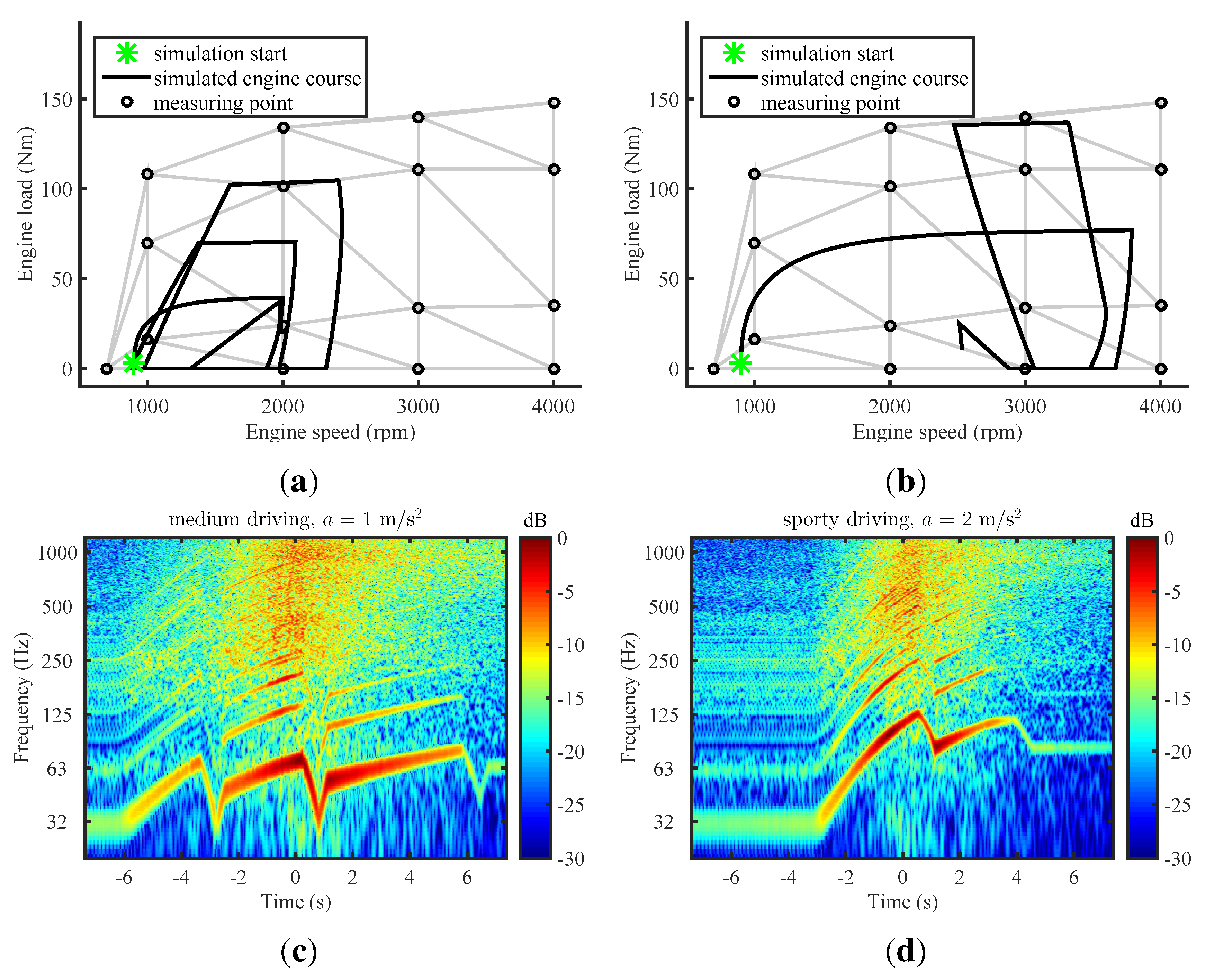
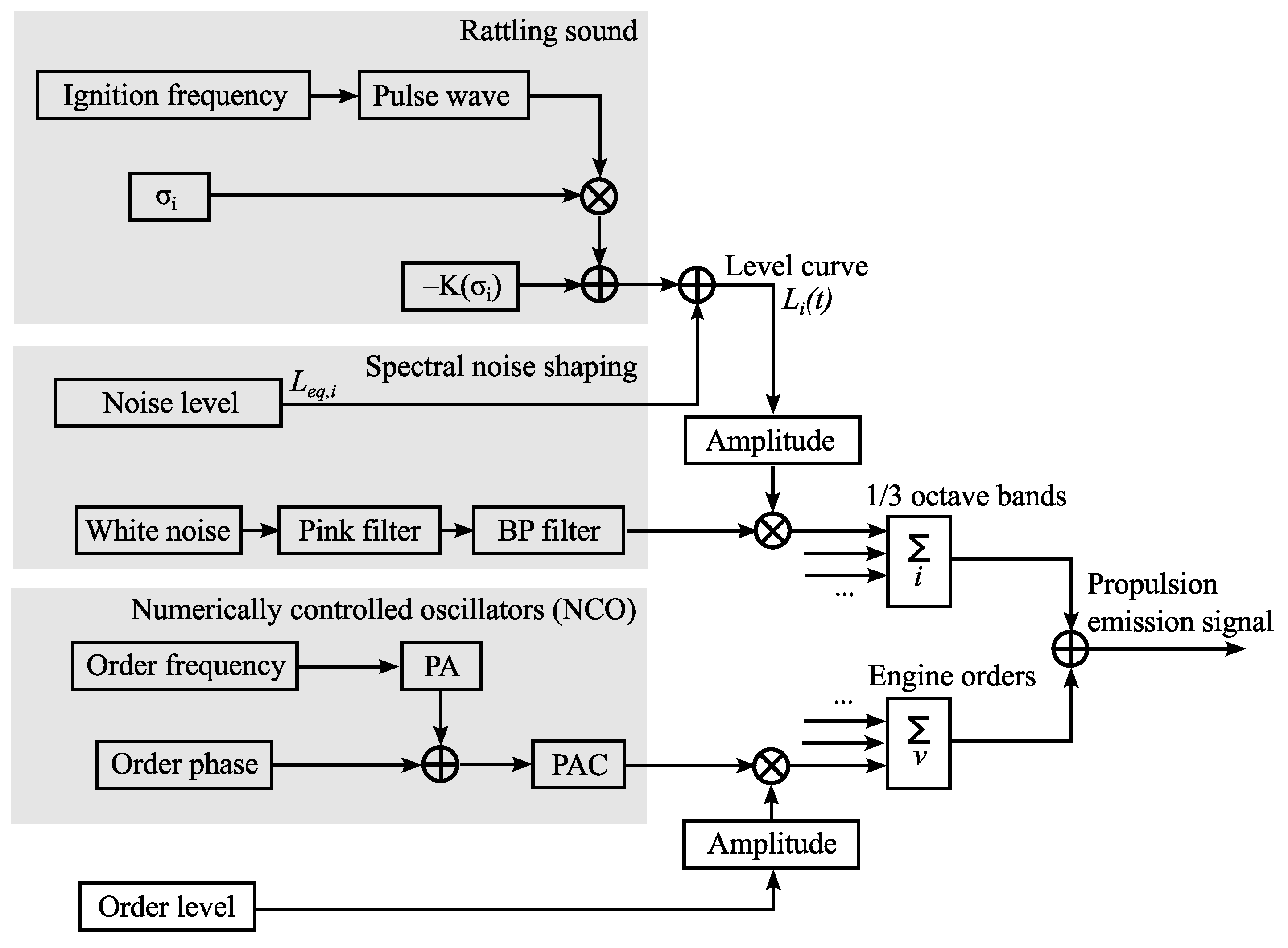
2.2.3. Sound of Propulsion

The structure of the emission synthesizer for the sound of propulsion is depicted in Figure 4. The sound pressure emission signal of the sound of propulsion is assumed to consist of a deterministic signal representing the most important engine orders and a quasi-stochastic signal:

$$s_{\mathrm{prop}}\left(t\right)=s_{\mathrm{prop},\mathrm{ord}}\left(t\right)+s_{\mathrm{prop},\mathrm{noise}}\left(t\right)$$

(13)

Engine order ν corresponds to an event taking place ν times per engine revolution. The engine order signal is composed of the sum of the engine orders ν, which are generated using additive synthesis [29,30]. The engine order signal is thus calculated by [6]:

$$s_{\mathrm{prop},\mathrm{ord}}\left(t\right)=\sum _{\nu }{p}_0{10}^{L_{\mathrm{prop},\mathrm{ord},\nu }^{†}\left(t\right)/20}·\sqrt{2}cos\left({\beta }_{\nu }\left(t\right)\right)$$

(14)

A proper selection of the essential orders ν strongly depends on the specific vehicle type and its condition. In the context of sound design, it is known that at least orders up to $\nu =18$ are relevant [23]. Further, the sound characteristics can be influenced by half-orders [23]. In this model, it was decided to synthesize orders $\nu =1$ to 30 in half-order steps, resulting in a total of 59 orders. This somewhat arbitrary, but safe choice leaves room for optimization. In Equation (14), $L_{\mathrm{prop},\mathrm{ord},\nu }^{†}$ denotes the order level and the instantaneous order phase:

$${\beta }_{\nu }\left(t\right)={\varphi }_{\nu }^{†}\left(t\right)+2\pi {\int }_{-\infty }^t{F}_{\nu }\left(\tau \right)d\tau$$

(15)

with the order phase ${\varphi }_{\nu }^{†}$ and the order frequency:

$$F_{\nu }\left(t\right)=\nu ·n\left(t\right)/60.$$

(16)

Listening tests revealed that in this application, the order phase is a relevant synthesizer parameter. For a four-stroke engine with $N_{\mathrm{cyl}}$ cylinders, the engine order corresponding to the ignition, and mostly the predominant order, is ${\nu }_{\mathrm{ign}}=N_{\mathrm{cyl}}/2$ [23]. Thus, the ignition frequency reads [5]:

$$F_{\mathrm{ign}}\left(t\right)=N_{\mathrm{cyl}}/2·n\left(t\right)/60.$$

(17)

Figure 4. Signal flow chart of the synthesizer for the sound of propulsion.

Figure 4. Signal flow chart of the synthesizer for the sound of propulsion.

For time-discrete signals, Equations (14) and (15) can be interpreted as a modified numerically-controlled oscillator (NCO) [28], whereas Equation (15) corresponds to the phase accumulator (PA), and the phase-to-amplitude converter (PAC) is realized in Equation (14). This formulation concurrently implements a frequency modulation by F and a phase modulation by $\varphi$.

The noise signal component of the sound of propulsion is synthesized similarly as the sound of tires (Equation (3)) by:

$$s_{\mathrm{prop},\mathrm{noise}}\left(t\right)=\sum _{i=1}^{N_b}{p}_0{10}^{L_{\mathrm{prop},\mathrm{noise},i}\left(t\right)/20}·{\xi }_i^{\prime }\left(t\right)$$

(18)

A total of $N_b=29$ bands from 20 Hz to 12.5 kHz are used. The 1/3 octave band level function is formulated as:

$$L_{\mathrm{prop},\mathrm{noise},i}\left(t\right)=L_{\mathrm{eq},\mathrm{prop},\mathrm{noise},i}^{†}+{\sigma }_i^{†}·R\left(t\right)-K\left({\sigma }_i^{†}\right)$$

(19)

with the level $L_{\mathrm{eq},\mathrm{prop},\mathrm{noise},i}^{†}$, a level standard deviation ${\sigma }_i^{†}$ and a level fluctuation function $R\left(t\right)$ with zero mean and unit power. The constant K ensures that despite the level fluctuations, the equivalent continuous level (Leq) is not altered. This level modulation simulates the rattling sound component that elicits a roughness sensation, which is particularly characteristic for low engine speeds and diesel engines. Motivated by measurement data that showed the strongest level fluctuations at the ignition frequency, R is modeled by a quasi-periodic function with period $1/F_{\mathrm{ign}}\left(t\right)$. The first half-period of R is composed of a Hann window, whereas the second half-period is held constant.

In summary, the presented synthesizer needs about 180 input parameters to generate a stationary signal for the sound of propulsion. However, during a pass-by, the sound of propulsion may considerably vary, and so do these parameters. These parameters, which are marked by † in the above equations, simultaneously depend on the engine speed n, the engine load M and the emission angle $\phi$ and are hence time dependent. They are calculated by a triangulation-based linear 3D interpolation of measurement data. Measurements were taken on a discrete grid, typically $n\approx \{1000,2000,3000,4000\}$ rpm, $\Gamma \approx \{0,40,70,100\}$% and $\phi ={\{0,60,120,180\}}^{\circ }$. The measuring point pairs $〈n,M〉$ of a measurement performed on a Ford Focus 1.8i are depicted as circles in Figure 3. The topmost points at 1000 to 4000 rpm are at full load, i.e., $\Gamma =100$%. Furthermore, the adopted Delaunay triangulation, which is used for the interpolation, is shown with gray lines. The synthesizer parameters are evaluated with a temporal resolution of 20 ms and linearly interpolated to the audio sampling rate, $f_s$. For the interpolation of the order phase, $\varphi$, its cyclic behavior has to be considered in order to avoid spurious phase fluctuations.

2.3. Propagation Filtering

The sound propagation model described in this section incorporates the following effects:

• Propagation delay
• Doppler effect (frequency shift and amplification)
• Convective amplification
• Geometrical spreading
• Ground reflection
• Air absorption

Other outdoor sound propagation effects that may be relevant in certain situations are screening [37,38,39], foliage attenuation [38], meteorological effects due to an inhomogeneous atmosphere [38,39,40,41,42], as well as reflections at artificial [38,43] and natural surfaces [42,44,45]. Most published environmental noise auralization models simulate some of the above listed effects by applying a 1/3 octave filter bank and adjusting the filter gains [8,14,15]. In this model, however, all of these effects are applied in the time domain, i.e., by time-variant digital filters. Sound propagation is modeled by two paths, namely for direct sound and a single ground reflection (in the following account indicated by subscripts “dir” and “gr”, respectively). The sound pressure of a point source has a $1/r$ distance dependency. Thus, to model geometrical spreading, the emitted sound pressure signals, x, are divided by their path length $r_{\mathrm{dir}}$ or $r_{\mathrm{gr}}$, respectively. The interaction of a sound wave with the ground influences its amplitude and phase as a function of frequency. This effect can be modeled by convolution of the ground-reflected signal with a time-variant filter [46]. Furthermore, the attenuation due to air absorption can be efficiently modeled using a filter [46]. Considering these aspects, the receiver signal y is calculated by:

$$y\left(t^{\prime }\right)=h_{\mathrm{air},t^{\prime }}\left(t^{\prime }\right)*\left(\frac{x_{\mathrm{dir}}\left(t^{\prime }\right)}{r_{\mathrm{dir}}\left(t^{\prime }\right)}+h_{\mathrm{gr},t^{\prime }}\left(t^{\prime }\right)*\frac{x_{\mathrm{gr}}\left(t^{\prime }\right)}{r_{\mathrm{gr}}\left(t^{\prime }\right)}\right)$$

(20)

where * denotes linear convolution, $t^{\prime }$ the receiver time axis, $r_{\mathrm{dir}}$ is the source–receiver distance, $r_{\mathrm{gr}}$ is the distance source–ground reflection point–receiver, $x_{\mathrm{dir}}$ and $x_{\mathrm{gr}}$ are delayed versions of the emitted sounds and $h_{\mathrm{air},t^{\prime }}$ and $h_{\mathrm{gr},t^{\prime }}$ denote impulse responses of time-dependent filters described in Section 2.3.2 and Section 2.3.3. The modeling of effects due to source motion and the propagation delay are explained in Section 2.3.1. Note that the immission angle $\theta \left(t^{\prime }\right)$, which is needed for surround reproduction, has to be evaluated on the receiver axis, as well.

Figure 3 shows normalized spectrograms of two synthesized pass-by sounds. For the synthesis of the sound of propulsion, the respective engine condition courses depicted in a and b of Figure 3 were used. They are described in Section 2.2.2. The temporal behavior of the engine states, the spectrograms, as well as the auralizations are published as supplementary data (see the videos in the Supplementary File). In both simulations, the car passes the receiver at Time 0 at 30 km/h. The receiver is located 1.2 m above a hard ground at a distance $D=7.5$ m. As at the pass-by, the engine speed still increases, the Doppler frequency shift is not directly observable in the course of the order frequencies. However, the gear change moments can be well observed as local decreases of order frequencies. As a consequence of the used engine condition courses, these frequency drops occur at higher frequencies for the sporty driving style (d).

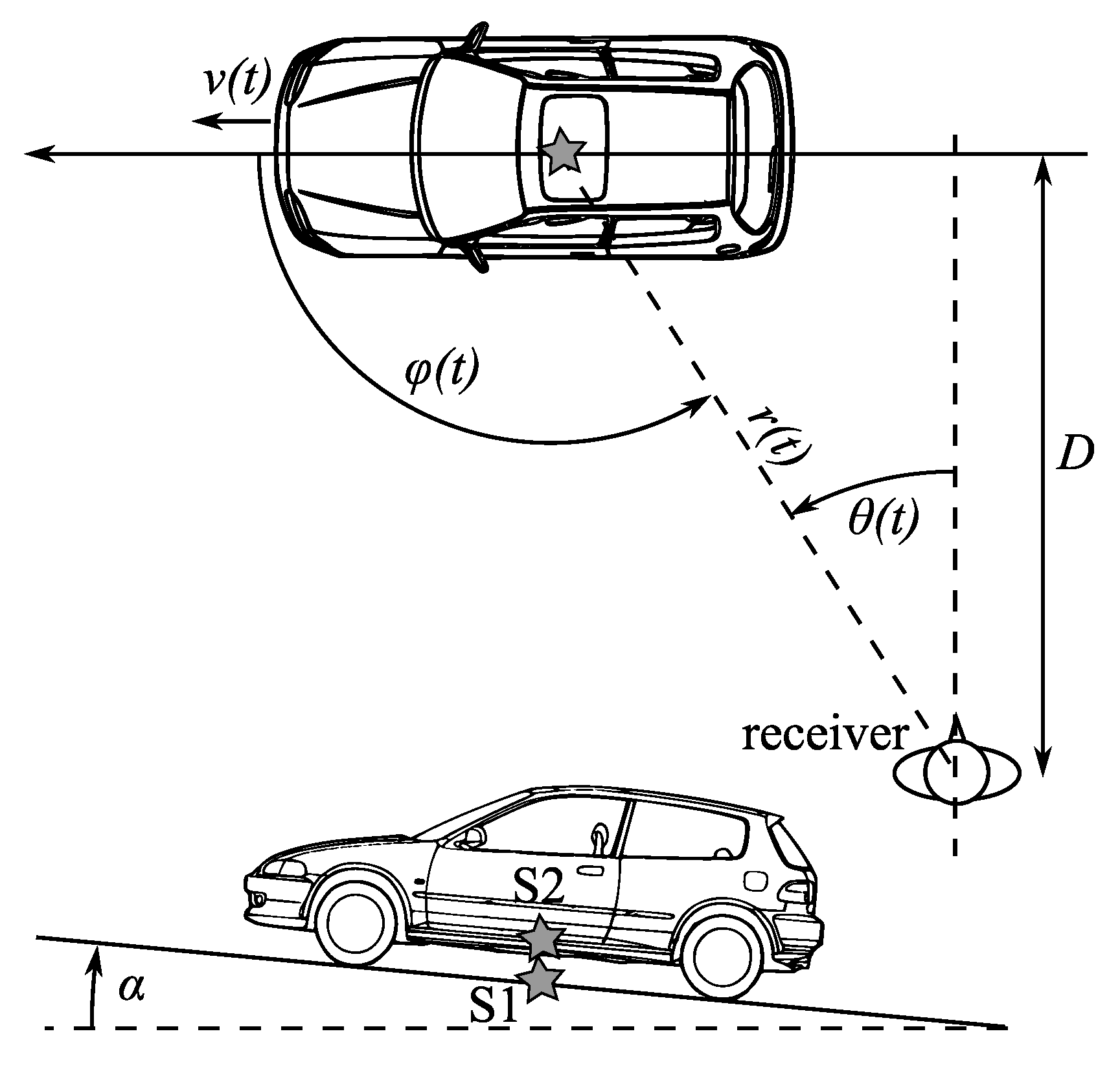
2.3.1. Effects Due to Source Motion and Propagation Delay

Due to the travel time of sound and the movement of the source, the source and the receiver have differing time axis. By neglecting wind and turbulence, the warped time axis at the receiver is given by:

$$t^{\prime }=t+\Delta t\left(t\right)=t+\frac{r_{\mathrm{dir}/\mathrm{gr}}\left(t\right)}{c_0}$$

(21)

where $r_{\mathrm{dir}/\mathrm{gr}}$ denotes the sound propagation distance of the direct sound or the ground reflected sound, respectively, and $c_0$ is sound speed in still air. A constant sound speed of $c_0=340$ m/s is assumed. Since the receiver signal is supposed to have a constant sampling rate of $f_s$, the corresponding times, $t_s$, on the emission time axis have to be found. This is achieved by linear interpolation of Equation (21). The emission signals x for the direct and the ground-reflected path, respectively, with respect to the receiver time $t^{\prime }$ are:

$$x_{\mathrm{dir}/\mathrm{gr}}\left(t^{\prime }\right)=s\left(t\right)·{\mathcal{D}}^2\left(t\right)$$

(22)

with the Doppler factor:

$$\mathcal{D}\equiv \frac{f^{\prime }}{f}=\frac{dt}{d{t}^{\prime }}.$$

(23)

Equation (22) describes the kinematic and the aerodynamic effect of source motion. The former is known as the Doppler effect, i.e., the Doppler frequency shift and amplification. The latter is known as convective amplification. The exponent two of the Doppler factor indicates that a Lighthill [47] monopole [48] and/or dipole source [49] is assumed.

The change of the time axis in Equation (22) realizes the propagation delay, as well as the Doppler frequency shift. For digital signals, this change corresponds to an asynchronous resampling process. It can by implemented using a variable delay-line with delay $\Delta t$ [50]. If $\Delta t$ is just rounded to the nearest sample, audible artifacts occur, so-called “zipper noise”. Therefore, an interpolation strategy has to be used. As we are only interested in sequential access to the emission signal, a fractional delay filter can be used [51]. In [18] and [50], a linear interpolator is proposed. This however produces high frequency attenuation, as well as strong nonlinear distortions due to aliasing. Therefore, here, we introduce a band-limited interpolation or, respectively, a windowed sinc interpolation [51]:

$$s\left(k_s\right)=\sum _{k=⌊k_s⌋-b+1}^{⌊k_s⌋+b}s\left[k\right]K\left(\left|k_s-k\right|\right)$$

(24)

with the floor function $⌊.⌋$, the integer sample index k, the non-integer sample index $k_s=t_s{f}_s$ and the Hamming kernel:

$$K\left(m\right)=\left\{\begin{array}{cc}\left[0.54+0.46cos(\pi m/b)\right]\mathrm{sinc}\left(m\right)\hfill & \mathrm{if}0\le m<b\hfill \\ 0\hfill & \mathrm{otherwise}\hfill \end{array}\right.$$

(25)

with an integer b describing the filter length. To keep the computational effort low, in the implementation of Equation (24), values of the kernel K are stored in a look-up table. The Doppler factor $\mathcal{D}$ in Equation (22) is implemented by approximating the derivative in Equation (23) by finite differences as:

$$\mathcal{D}\left(k_{s,i}\right)\cong k_{s,i+1}-k_{s,i}.$$

(26)

with index i.

In order to validate different implementations of Equation (22), numerical simulations were performed. Figure 5 compares the signal attenuation introduced by different interpolation schemes. The high frequency attenuation of the linear interpolation can be improved by a windowed sinc interpolation and controlled by parameter b. Figure 6 shows spectrograms of receiver signals calculated by the same three interpolation schemes. As an extreme case, a virtual source emitting a 1 kHz pure tone travels at constant speed $v=150$ km/h and passes a static receiver at a distance of $D=7.5$ m. Figure 6 shows that by introducing a windowed sinc interpolation of sufficient filter length, artifacts due to aliasing can be significantly reduced compared to a linear interpolation (a). The minimal kernel size b required for a decent sound quality cannot be stated in general, as it strongly depends on the application, i.e., the source signal, the propagation situation and, not least, the sampling frequency. However, in the example of Figure 6, already, $b=10$ reaches a good sound quality, without audible artifacts. Nevertheless, to be on the safe side, a value of $b=100$ was adopted. The careful choice of b, however, provides the potential for optimization in terms of sound quality and computational cost.

For sound speed $c_0=340$ m/s, the Mach number $M\equiv v/c_0\approx 0.12$. At times $t=\pm \infty$, the received frequencies $f^{\prime }$ due to the Doppler shift are given by [2,52]:

$$f_{t=\pm \infty }^{\prime }=f·{\mathcal{D}}_{t=\pm \infty }=\frac{f}{1\pm M}$$

(27)

with f being the emitted frequency. In our example, according to Equation (27), the received frequency changes by a factor of 1.28 across the pass-by, which corresponds to a musical interval that is larger than a major third. The sum of the Doppler and the convective amplification amounts to [48]:

$$G_{t=\pm \infty }=-40·log10\left(1\pm M\right)\left[\mathrm{dB}\right]$$

(28)

Equation (28) yields an amplification of 2.3 dB at $t=-\infty$ and an attenuation by 2.0 dB at $t=\infty$, resulting in a level difference of 4.3 dB across the pass-by. The numerical implementations of Equation (22) corresponded well with these theoretical values.

Figure 5. Spectral attenuation due to different resampling strategies.

Figure 5. Spectral attenuation due to different resampling strategies.

Figure 6. Non-linear distortions (aliasing) due to different resampling strategies: linear interpolation (a) and Hamming sinc interpolations with different filter lengths, $b=10$ for (b) and $b=100$ for (c), respectively. The simulation was performed for a source emitting a 1 kHz pure tone that travels at constant speed $v=150$ km/h and passes a static receiver at a distance of $D=7.5$ m.

Figure 6. Non-linear distortions (aliasing) due to different resampling strategies: linear interpolation (a) and Hamming sinc interpolations with different filter lengths, $b=10$ for (b) and $b=100$ for (c), respectively. The simulation was performed for a source emitting a 1 kHz pure tone that travels at constant speed $v=150$ km/h and passes a static receiver at a distance of $D=7.5$ m.

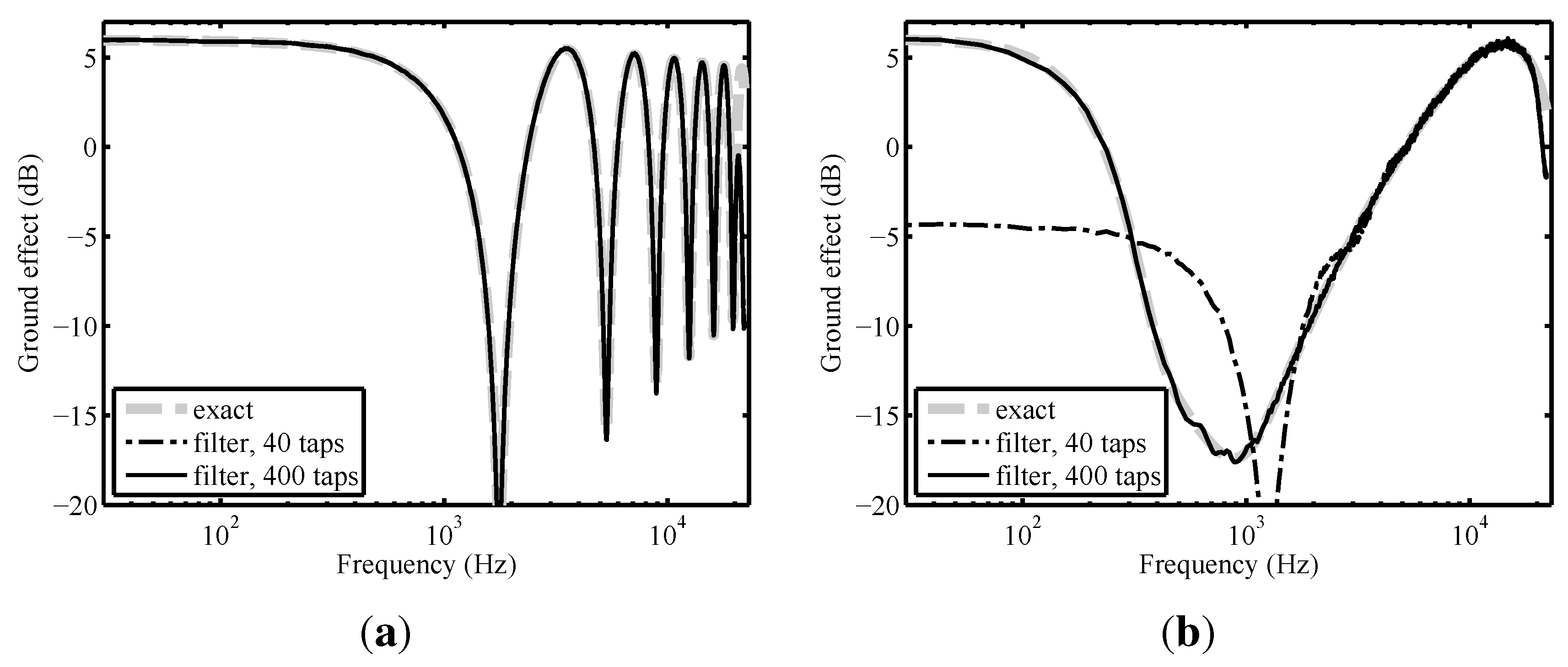
2.3.2. Ground Effect

In Equation (20), the ground effect is modeled in a physical way as the interference between direct and ground reflected sound. A flat topography is assumed, i.e., only one ground-reflected path is modeled, which is implemented by adding a second signal path. The ground-reflected sound differs from direct sound by scaling with its propagation distance and a complex reflection factor, as well as an additional delay. The complex reflection factor depends on frequency, geometry and ground surface type and is realized by the filter $h_{\mathrm{gr},t^{\prime }}$. $h_{\mathrm{gr},t^{\prime }}$ is the impulse response of the spherical wave reflection coefficient at an infinite locally-reacting surface. The ground surface is acoustically described by a frequency-depending surface impedance, for which the widely-used empirical model of Delany and Bazley [53] was used.

In [46], the additional delay of the ground-reflected sound was modeled by a digital delay of integer length. However, in this application, due to the higher relative source speed and short delays, audible artifacts (“zipper noise”) occur. Therefore, a separate resampling is performed in Equation (22) for the ground-reflected sound. Furthermore, this type of processing eliminates the spectrally-fluctuating errors (see Figure 1 in [46]).

The spherical wave reflection coefficient filter $h_{\mathrm{gr},t^{\prime }}$ is implemented by an FIR filter designed using the inverse FFT, as described in [46]. It has to be made sure that the filter lag is compensated. However, compared to [46] for this application, substantially more filter taps are required to reproduce the correct interference pattern. Figure 7 shows simulation results for the standard configuration of road traffic noise emission measurements (a) and a receiver point at distance $D=100$ m and height 2 m with sound propagation over grassy ground (b). For the former case a filter with 40 taps is sufficient, as the difference to the simulation with a filter with 400 taps stays well below 1 dB for all frequencies (nearly perfect coincidence of curves in Figure 7a). For the latter case, however, Figure 7b shows that such a short filter is not able to correctly reproduce the interference pattern and creates large errors at mid and low frequencies. A filter length of 400 taps allows simulations that are in good agreement with the exact solution for both cases. Large errors only occur near the Nyquist frequency. An update interval of the filter coefficients of 200 ms is used.

Figure 7. Simulated ground effect spectra for a point source at a height of 0.3 m in the reference situation (a) with a receiver at a height of 1.2 m at a horizontal distance of $D=7.5$ m and propagation over hard ground (flow resistivity 20,000 kPa·s·m${}^{-2}$); and a distant situation (b) with a receiver at a height of 2 m at horizontal distance $D=100$ m and propagation over grassy ground (flow resistivity 200 kPa·s·m${}^{-2}$).

Figure 7. Simulated ground effect spectra for a point source at a height of 0.3 m in the reference situation (a) with a receiver at a height of 1.2 m at a horizontal distance of $D=7.5$ m and propagation over hard ground (flow resistivity 20,000 kPa·s·m${}^{-2}$); and a distant situation (b) with a receiver at a height of 2 m at horizontal distance $D=100$ m and propagation over grassy ground (flow resistivity 200 kPa·s·m${}^{-2}$).

2.3.3. Air Absorption

For performance reasons, the identical air absorption filter $h_{\mathrm{air},t^{\prime }}$ is applied to the direct and ground reflected path in Equation (20). $h_{\mathrm{air},t^{\prime }}$ are linear-phase FIR filters designed using the inverse FFT, as described in [46]. The frequency-dependent sound attenuation coefficients for atmospheric absorption as a function of relative humidity and temperature are calculated according to the standard ISO 9613-1 [54]. A filter length of 30 taps is used with an update interval of the filter coefficients of 200 ms.

2.4. Reproduction Rendering

The rendering of the immission signals for reproduction strongly depends on the type of reproduction system. For surround reproduction via multiple loudspeakers, techniques, such as Ambisonics [55,56] or amplitude panning (e.g., Vector Base Amplitude Panning (VBAP) [57] or Multiple-Direction Amplitude Panning (MDAP) [58]), are possible candidates. For binaural reproduction over headphones, generally, head-related transfer functions (HRTF) should be applied. In this paper, for simplicity, a simulation of the “ORTF” stereo technique [59,60] is used. If the listener is facing the road, this allows for a reproduction with sufficient accuracy via headphones and a stereo speaker set-up. The cardioid microphone pattern and the time difference between the left and right channel are modeled by:

$$\begin{array}{ccc}\hfill L\left(t^{\prime }\right)& =& 0.5\left(1+cos(\theta -{55}^{\circ })\right)·y(t^{\prime }+u)\hfill \end{array}$$

(29)

$$\begin{array}{ccc}\hfill R\left(t^{\prime }\right)& =& 0.5\left(1+cos(\theta +{55}^{\circ })\right)·y\left(t^{\prime }\right)\hfill \end{array}$$

(30)

with the time-varying time difference:

$$u=\frac{0.17·sin\left(\theta \left(t^{\prime }\right)\right)}{c_0}$$

(31)

The immission angle $\theta \left(t^{\prime }\right)$ has to be evaluated on the receiver axis (see Equation (21)). $y(t^{\prime }+u)$ is calculated using a windowed sinc interpolation strategy according to Equation (24). As a consequence of this interpolation, high-frequency attenuation, as shown in Figure 5, and nonlinear distortions are introduced to channel L.

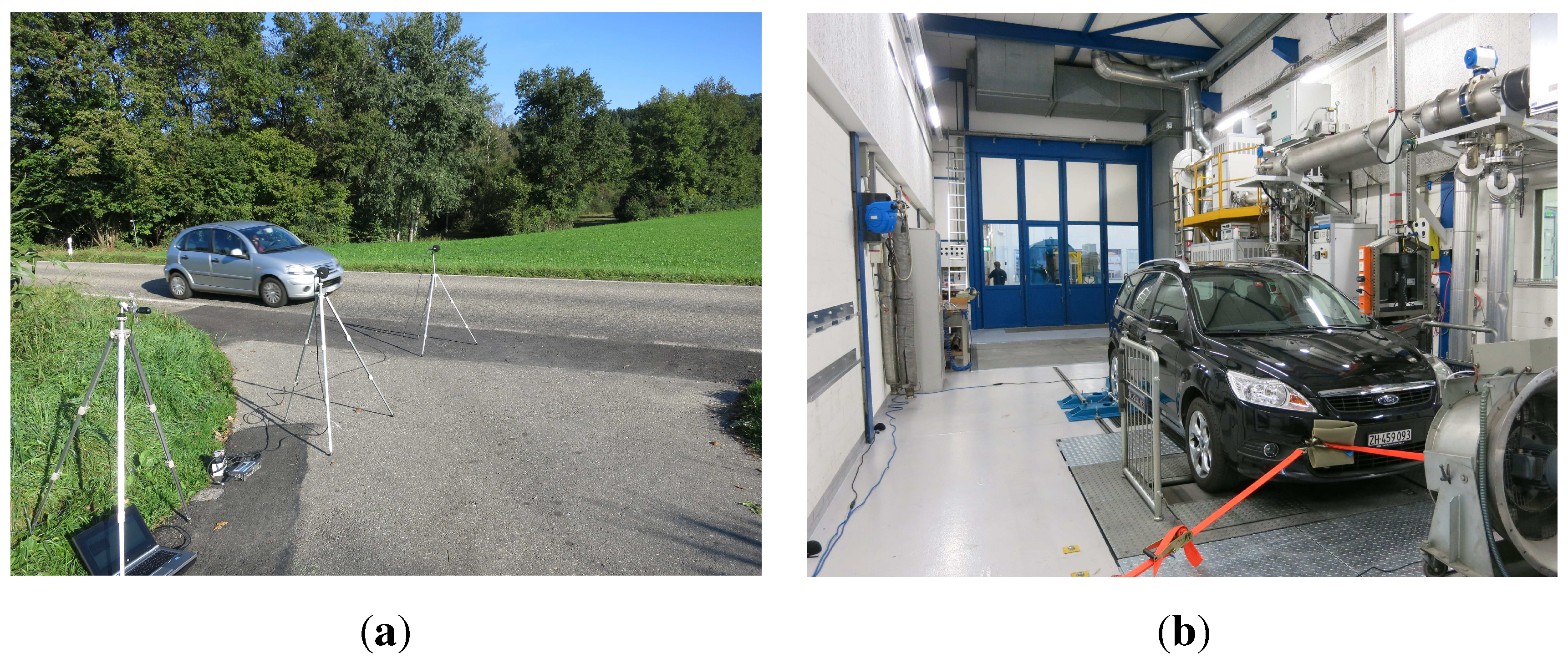
3. Model Parameter Estimation

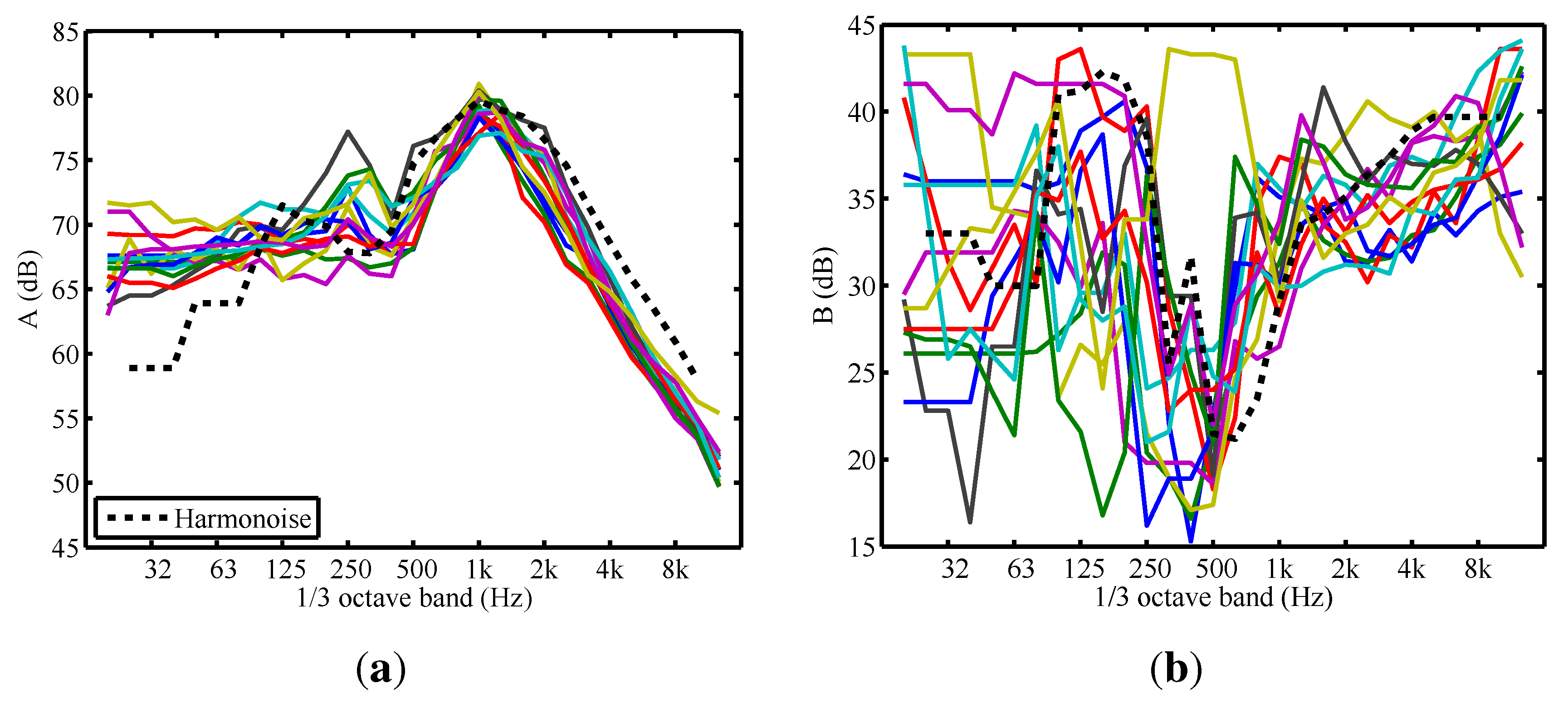
This section presents procedures to obtain the model parameters of the emission synthesizer described in Section 2.2. The procedures are based on controlled measurements. The following sections describe the measurements, as well as the signal processing that is applied to the acquired data.

3.1. Tire Noise

The emission parameters for tire noise were obtained from pass-by measurements with idling engine. For an individual tire type, pass-bys by the same passenger car at different speeds were recorded at a sampling frequency of $f_s$ = 44.1 kHz with a calibrated measurement microphone in a set-up referring to the standard ISO 11819-1 [25] and depicted in Figure 8a. The pass-by speed was measured by radar, and the pass-by time was determined from synchronous video. Under the assumption of constant speed, a time-dependent backpropagation to the source was performed. Thereby, two equal incoherent point sources at the nearby wheels were assumed, i.e., placed at the side of the car, horizontally separated by the wheelbase and set on the ground. For the temporal accordance, the sound propagation delay, as well as the filter group delays of the 1/3 octave band filters have to be taken into account. Consequently, emission levels at reference distances $r_0$ were obtained by integration over an emission angle range of 90${}^{\circ }$. Applying a logarithmic transformation to the measured pass-by speeds, the linear regression parameters $A_i$ and $B_i$ of Equation (4) were fitted in a least-squares sense. Despite the idling engine, some low 1/3 octave bands were contaminated by the engine sound. To correct for this, in the first step, for each band, a quality criterion based on the correlation coefficient and the slope of the regression line was deployed. Adverse bands were identified and imputed based on the values of adjacent valid bands. In the second step, low-frequency peaks of $A_i$ were smoothed by a nonlinear method. Figure 9 contains measured parameters A and B in 1/3 octave bands of 13 tires.

Figure 8. Photographs showing the measurement set-ups for tire noise (a) and propulsion noise (b). In (a), the coast-by situation is depicted with two measurement microphones placed at different distances and a camera connected to a laptop; (b) shows the lab with a passenger car on the chassis dynamometer, the airstream fan in front of the car and two microphones on the floor at the left-hand room edge (emission angles $\phi ={60}^{\circ }$ and 120${}^{\circ }$).

Figure 8. Photographs showing the measurement set-ups for tire noise (a) and propulsion noise (b). In (a), the coast-by situation is depicted with two measurement microphones placed at different distances and a camera connected to a laptop; (b) shows the lab with a passenger car on the chassis dynamometer, the airstream fan in front of the car and two microphones on the floor at the left-hand room edge (emission angles $\phi ={60}^{\circ }$ and 120${}^{\circ }$).

Figure 9. Measured tire noise regression parameters $A_i$ (a) and $B_i$ (b) of 13 tires and the values according to the Harmonoise model [21] (dotted lines).

Figure 9. Measured tire noise regression parameters $A_i$ (a) and $B_i$ (b) of 13 tires and the values according to the Harmonoise model [21] (dotted lines).

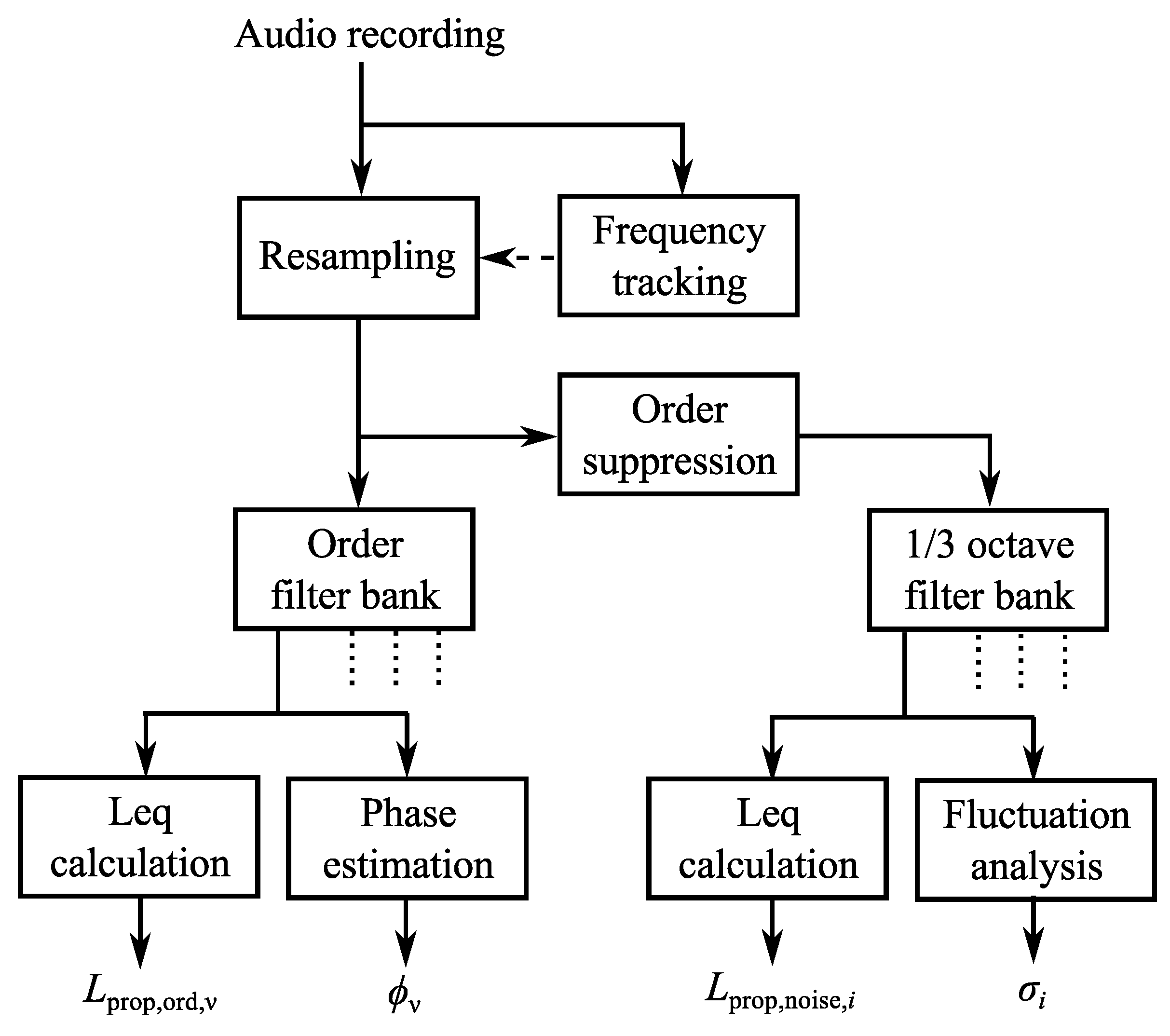
3.2. Propulsion Noise

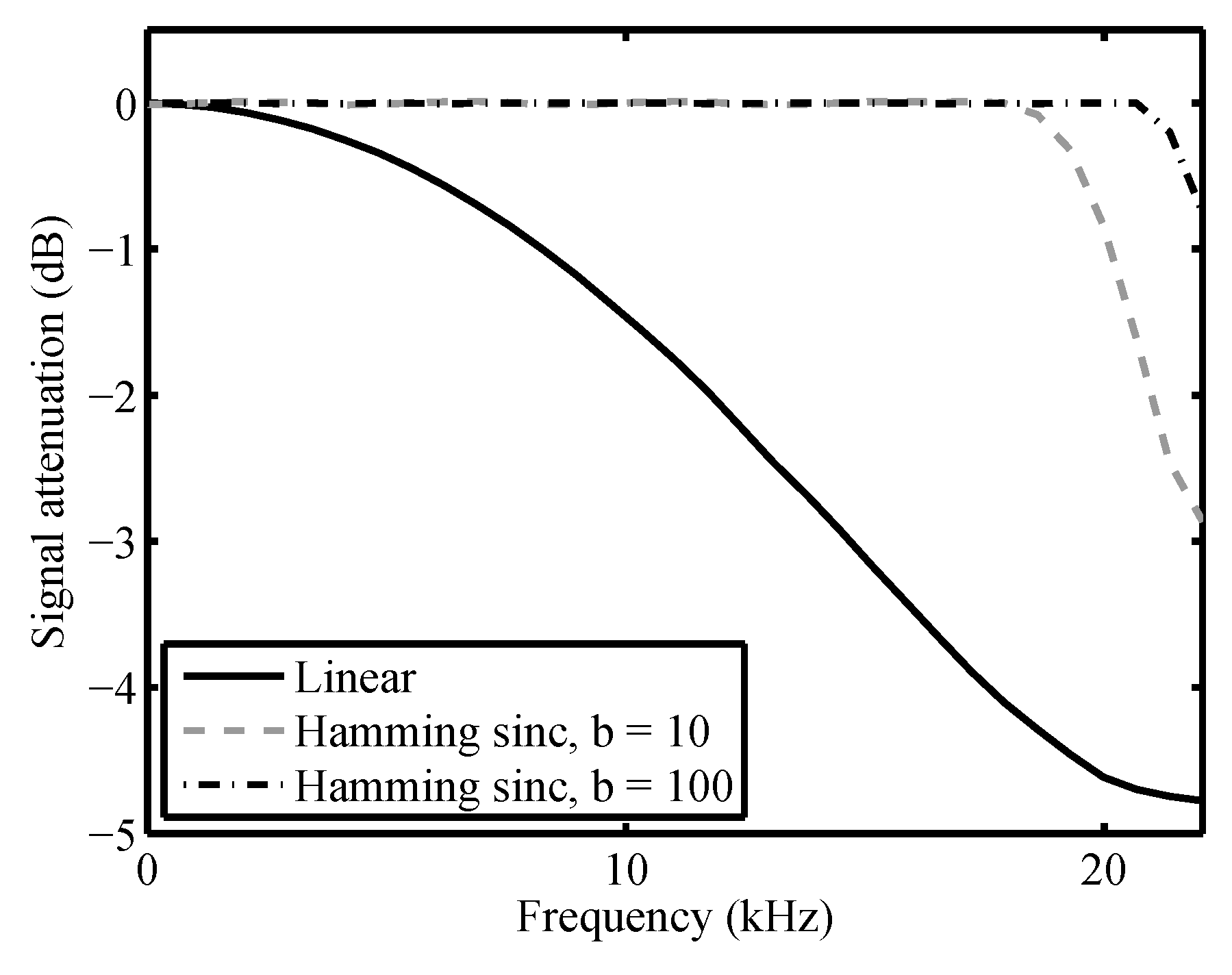
To obtain the emission synthesizer parameters of the propulsion noise, controlled measurements on a chassis dynamometer (see Figure 8b) and at idling engine under free field conditions were performed. Calibrated audio recordings at a sampling frequency of $f_s$ = 44.1 kHz at different microphone positions around the vehicle and at different engine conditions were taken. During the measurements on the chassis dynamometer, four microphones were placed on the ground at emission angles $\phi \approx {\{0,60,120,180\}}^{\circ }$ at distances r = 1 to 2 m from the vehicle. During the free field measurements, four additional microphones were placed on the ground at the identical emission angles, but at larger distances of $r^{\prime }$ = 4.5 to 7 m. The free field measurements were used to correct for the room influences of the lab, as explained in Section 3.2.5. On the chassis dynamometer, measurements were typically taken at engine speeds of $n\approx \{1000,2000,3000,4000\}$ rpm and engine loads of $\Gamma \approx \{0,40,70,100\}$%. The measuring point pairs $〈n,M〉$ of a measurement performed on a Ford Focus 1.8i are depicted as circles in Figure 3. The topmost points at 1000 to 4000 rpm are at full load, i.e., $\Gamma =100$%. To confine tire noise, low vehicle speeds were aimed for by choosing low driving gears. Mostly, it was the second gear, which resulted in vehicle speeds <50 km/h.

To these recordings, a series of signal analysis steps were applied, which are outlined in a signal flowchart in Figure 10. These steps are further explained in the following sections. For the signal processing, a signal length of 4 s is used.

Figure 10. Signal analysis flowchart to obtain the synthesizer parameters of propulsion noise as described in Section 2.2.3 from audio recordings.

Figure 10. Signal analysis flowchart to obtain the synthesizer parameters of propulsion noise as described in Section 2.2.3 from audio recordings.

3.2.1. Resampling

The emission synthesizer uses detailed information about the engine orders. These parameters are obtained by a narrowband analysis, which is described in the following section. Although during the measurements, the engine speed was kept fairly constant, the instantaneous order frequencies slightly fluctuate as exemplarily shown in Figure 11. This figure shows the spectrogram of a recording made at the rear of a car with an inline, four cylinder engine idling at 1100 rpm. To be able to separate engine orders and broadband noise by the narrowband analysis, a preceding resampling of the slightly non-stationary signals is performed. In order to actuate the resampling process, the instantaneous ignition frequency, $F_{\mathrm{ign}}\left(t\right)$, of the engine is required. This data are extracted from the audio recordings.

In the first step, the average ignition frequency is estimated. From the signal taken closest to the exhaust, the power spectral density (PSD) with a frequency resolution <1 Hz is calculated. Based on the rough indication of the engine speed taken from the car’s tachometer, a first estimate of the ignition frequency, $F_{\mathrm{ign}}$, is obtained using Equation (17). The location of the maximum value of the PSD within a search range around this frequency yields a better, second estimate. Particularly, for low engine speeds, at which the ignition frequency can be as low as 20 Hz, this estimate is still not precise enough due to the low relative resolution at low frequencies. Thus, this estimate is further enhanced by considering the double ignition frequency, $2F_{\mathrm{ign}}$, (i.e., engine order $\nu =4$ in Equation (16) for a four-cylinder engine) within a smaller range of the PSD.

Figure 11. Normalized spectrogram (a) of the measured sound pressure signal with tracked double ignition frequency (drawn as a black line) and power spectral density (b) of the original and asynchronously resampled sound pressure signal, respectively. The recording was conducted at the rear of the BMW with an inline, four-cylinder engine idling at 1100 rpm.

Figure 11. Normalized spectrogram (a) of the measured sound pressure signal with tracked double ignition frequency (drawn as a black line) and power spectral density (b) of the original and asynchronously resampled sound pressure signal, respectively. The recording was conducted at the rear of the BMW with an inline, four-cylinder engine idling at 1100 rpm.

In the second step, this information is used to track the course of the ignition frequency, $F_{\mathrm{ign}}\left(t\right)$. This task is generally known as pitch detection [61,62,63]. A wide variety of algorithms exist that work in the time or frequency domain or a combination of them. In our application, a spectral method was established, in which the course of one discrete frequency component (i.e., an engine order) is tracked in a spectrogram. The spectrogram $S(t,f)$ expressed in decibels is computed by the short-time Fourier transform (STFT):

$$S(t,f)=10·log\left({\left|STFT(t,f)\right|}^2\right).$$

(32)

STFT is calculated using the FFT. Windows of 200 ms with a 50% overlap, i.e., a temporal resolution of $\Delta t=100$ ms, are multiplied by a Hann window function. To obtain a high frequency resolution of $\Delta f<0.5$ Hz, the signals are zero padded. A section of such a spectrogram is depicted in Figure 11. Within the spectrogram, the “highest cost” path between time $t=0$ and $t=T$, within a certain frequency range around a reference frequency, $F_r$, is sought. $F_r$ is chosen to be the first multiple of the mean ignition frequency above 55 Hz. This is a compromise between signal power and frequency localization: typically, the power decreases for increasing even orders (see Figure 11b), but higher orders exhibit larger absolute frequency variations (see Figure 11a). In the example of Figure 11, $F_r$ is 71 Hz (corresponding to the fourth engine order), as the mean ignition frequency lies at 35 Hz.

The optimization task is solved by dynamic programming, which breaks the complex problem down into many simple subproblems. This method prevents taking possible wrong local decisions and guarantees that the best solution is found. A well-known algorithm that uses dynamic programming is dynamic time warping (DTW), which is often applied in, e.g., automatic speech recognition (ASR). Additionally, we make use of the a priori knowledge that the engine speed does not change rapidly over time. This is introduced as a requirement on the slope of the optimal path, $F_{\mathrm{opt}}$. The algorithm described below is based on an algorithm developed for object tracking in video data [64]. Within the search section of the discrete spectrogram, the local score q is calculated by:

$$q(m,l)=S\left(m,l\right)-\underset{m,l}{min}\left(S(m,l)\right)$$

(33)

for which holds $q\ge 0$. From q for each time step $m=\{1...M\}$ and frequency bin l, the global score $Q(m,l)$ is recursively computed by:

$$Q(m,l)=q(m,l)+\underset{l^{\prime }\in \left\{l-c\le l\le l+c\right\}}{max}Q(m-1,l^{\prime })$$

(34)

with a positive integer c realizing the requirement:

$$\left|C\right|\le c\frac{\Delta f}{\Delta t}$$

(35)

on the absolute value of the slope C of $F_{\mathrm{opt}}$ given in Hertz per second. For the forward processing described by Equation (34), the starting condition is that the initial global score, $Q(1,l)$, is set to the local score, i.e., $Q(1,l)=q(1,l)$. During the evaluation of Equation (34), it is essential that the back pointers:

$$B(m,l)=\underset{l^{\prime }\in \left\{l-c\le l\le l+c\right\}}{arg\; max}Q(m-1,l^{\prime })$$

(36)

to the optimal predecessors are stored. From the global score Q, the end point of the optimal path is found by:

$$F_{\mathrm{opt}}\left(M\right)=\underset{l}{arg\; max}Q(M,l).$$

(37)

Using the back pointers B, the optimal path can be traced back using a recursive procedure known as backtracking:

$$F_{\mathrm{opt}}(m-1)=B\left(m,F_{\mathrm{opt}}\left(m\right)\right)$$

(38)

In Appendix, we provide a simple MATLAB code, which solves Equations (34) to (38). Figure 11 shows the optimal path drawn as a black line following the frequency component around 70 Hz.

In the third step, the sound pressure signal is asynchronously resampled based on the course of the tracked engine order. The warped time axis is calculated by:

$$t_{\mathrm{warp}}=t+\frac{F_{\mathrm{opt}}\left(t\right)}{F_r}$$

(39)

where $F_{\mathrm{opt}}\left(t\right)$ is the linearly-interpolated version of $F_{\mathrm{opt}}\left(m\right)$. For the resampling of the sound pressure signals, a windowed sinc interpolation, as described by Equation (24), is adopted. Figure 11 illustrates the effect of the asynchronous resampling on the power spectral density. In contrast to the original signal, for the resampled signal, all even engine orders from two to 12 can be clearly identified as equidistant, narrow peaks.

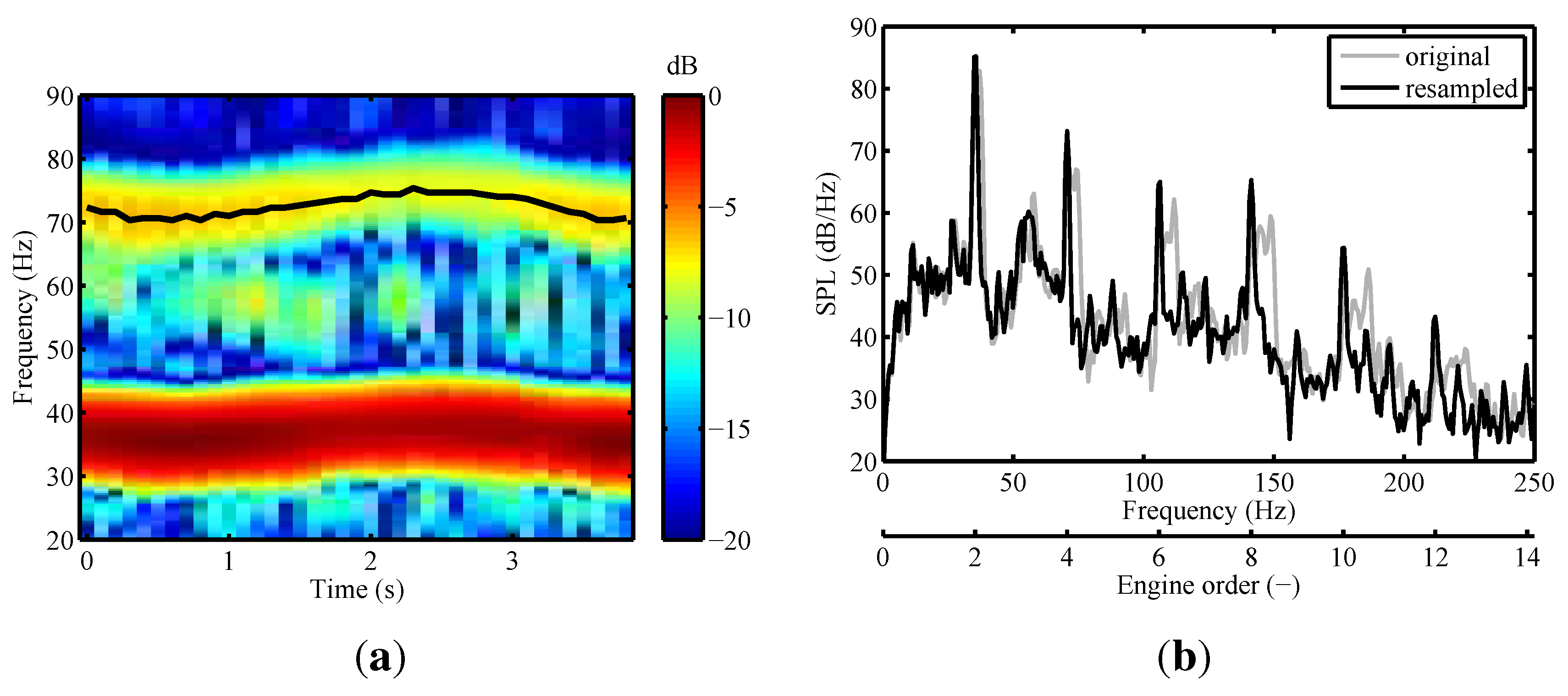
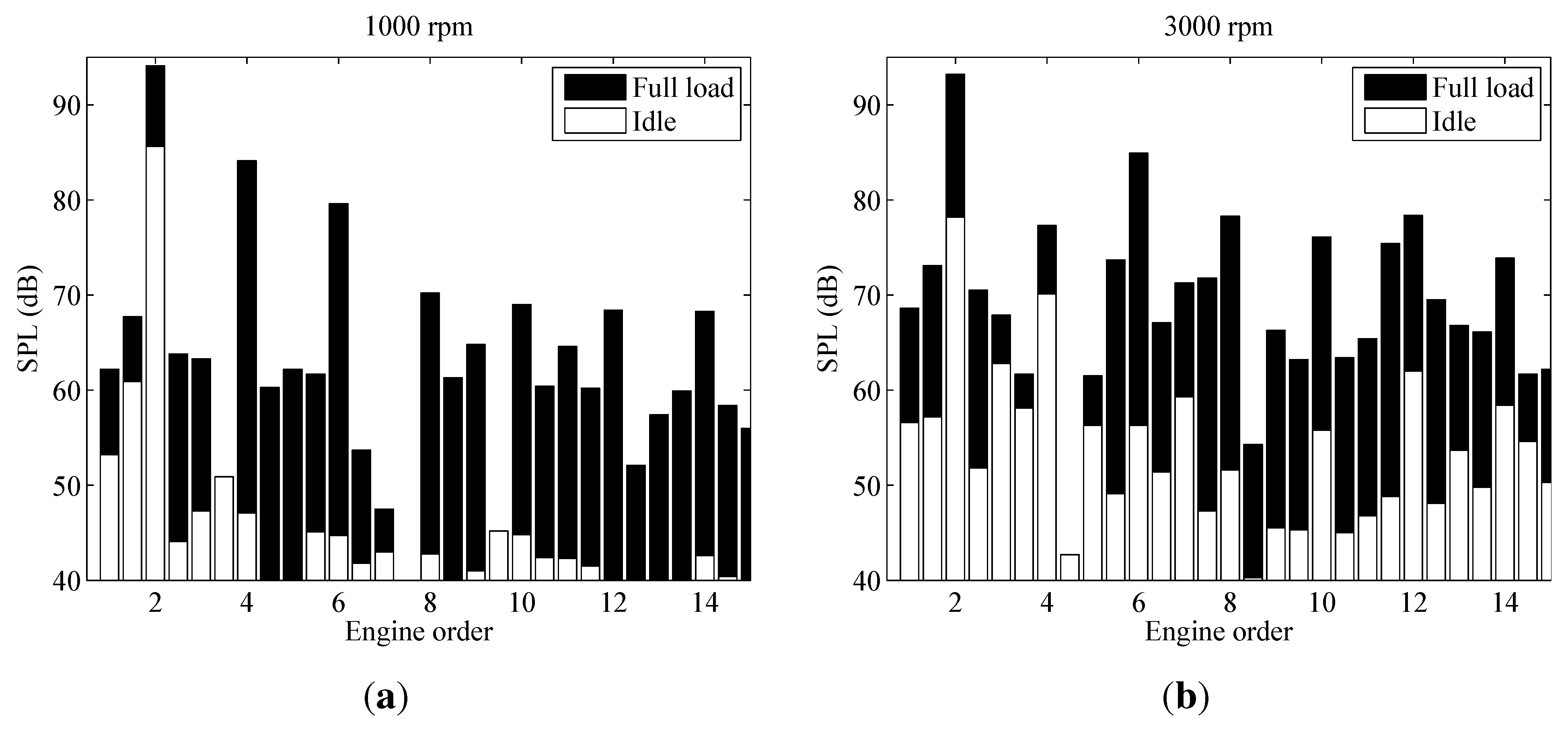
3.2.2. Order Analysis

From the resampled signals, information about the engine orders is extracted. Therefore, a filter bank consisting of one bandpass filter per considered engine order is generated and applied to the signal. Eighth order Butterworth filters centered around the engine order frequency $F_{\nu }$ with a 6-Hz bandwidth are employed. Figure 12 shows the magnitude frequency response of the filter bank. At the output of each filter, the corresponding order level, $L_{\mathrm{prop},\mathrm{ord},\nu }$ in Equation (14), is calculated as an equivalent continuous level (Leq). Figure 13 exemplifies measured order levels at idling engine and full load recorded at the rear of a VW Touran running at 1000 and 3000 rpm.

Figure 12. Magnitude frequency response of the engine order analysis filter bank (a) and engine order suppression filter (b) for engine speed $n=1000$ rpm, engine orders $\nu =1,1.5,2,...,15$ and $N_{\mathrm{cyl}}=4$.

Figure 12. Magnitude frequency response of the engine order analysis filter bank (a) and engine order suppression filter (b) for engine speed $n=1000$ rpm, engine orders $\nu =1,1.5,2,...,15$ and $N_{\mathrm{cyl}}=4$.

The order phases are detected using the cross-correlation function. Since the above-described infinite impulse response (IIR) filter bank introduces phase shifts, the outputs of the filter bank are time reversed and sent once again through the same filter bank and, finally, time reversed. In doing so, a zero-phase forward and reverse digital IIR filtering is implemented. This signal, $g_{\nu }\left(t\right)$, is cross-correlated with a prototype function $cos\left(2\pi F_{\nu }t\right)$ to obtain the time shift:

$${\kappa }_{\nu }=\underset{\tau }{arg\; max}\left\{\int g_{\nu }(t+\tau )cos\left(2\pi F_{\nu }t\right)dt\right\}$$

(40)

from which the phase shift of Equation (15) can be derived as:

$${\varphi }_{\nu }=-2\pi F_{\nu }{\kappa }_{\nu }.$$

(41)

Figure 13. Comparison of engine order levels with idling engine (white) and full load (black) at 1000 (a) and 3000 rpm (b). Recorded at the rear of a VW Touran 1.6 FSI.

Figure 13. Comparison of engine order levels with idling engine (white) and full load (black) at 1000 (a) and 3000 rpm (b). Recorded at the rear of a VW Touran 1.6 FSI.

Figure 14 compares the sound pressure signals of a recording and the corresponding synthesis consisting of engine orders with constant phases, which were estimated by Equation (41).

Figure 14. Comparison of sound pressure signals of a recording (a) and the corresponding synthesis consisting of engine orders with estimated phases (b). For the purpose of illustration only, the four dominant engine orders (colored lines) are used. The recording was conducted at the rear of a Ford Focus 1.8i at 1000 rpm and full load.

Figure 14. Comparison of sound pressure signals of a recording (a) and the corresponding synthesis consisting of engine orders with estimated phases (b). For the purpose of illustration only, the four dominant engine orders (colored lines) are used. The recording was conducted at the rear of a Ford Focus 1.8i at 1000 rpm and full load.

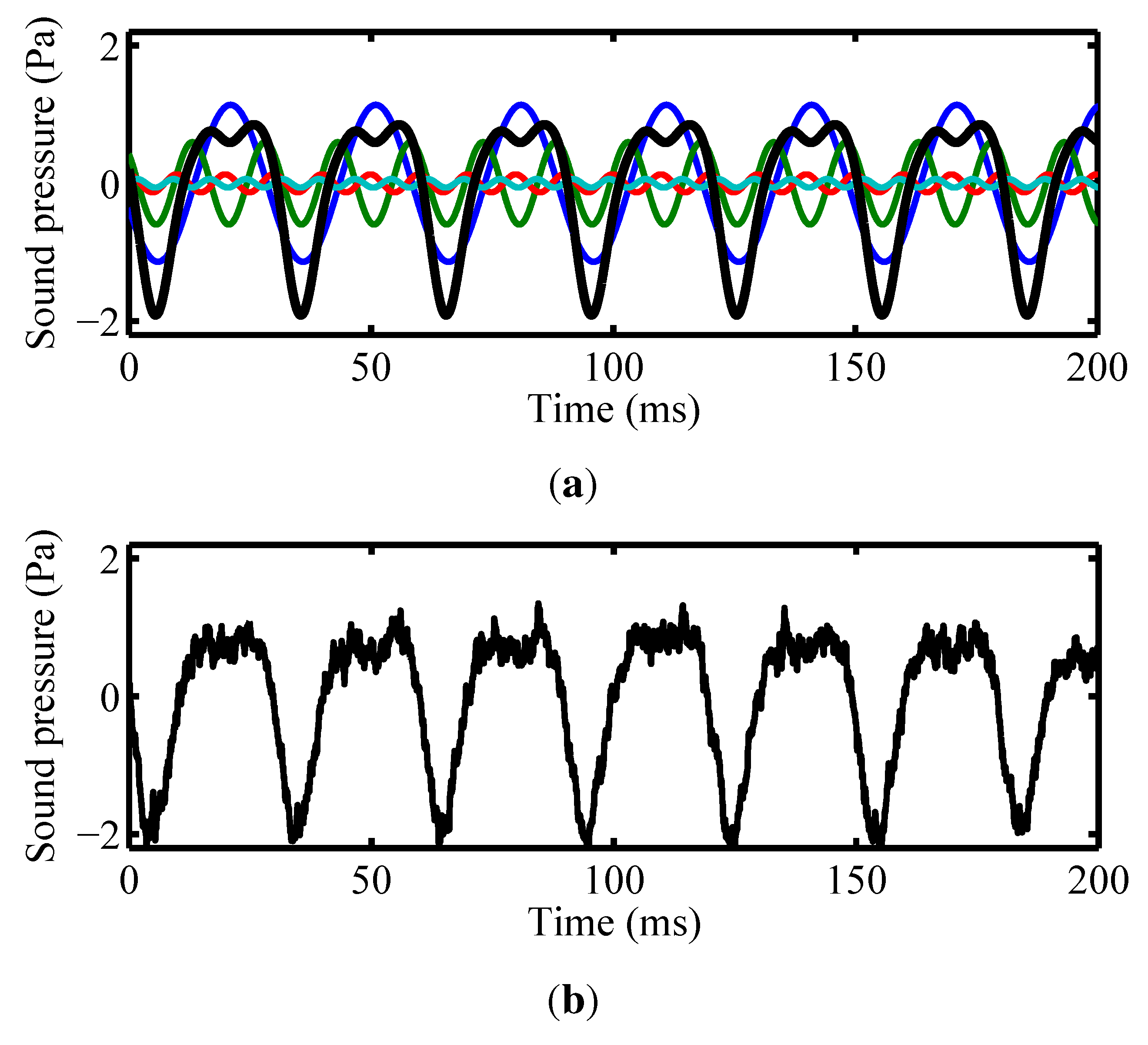
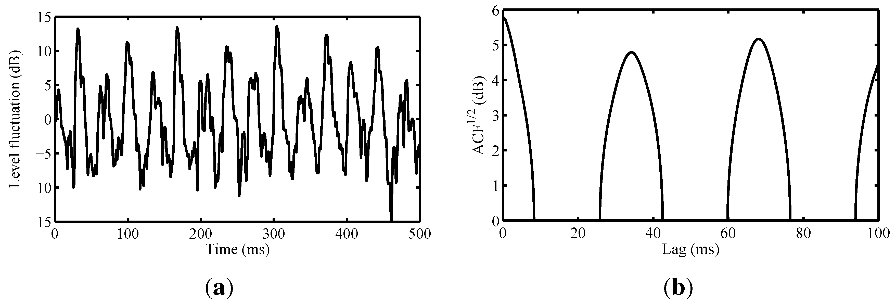
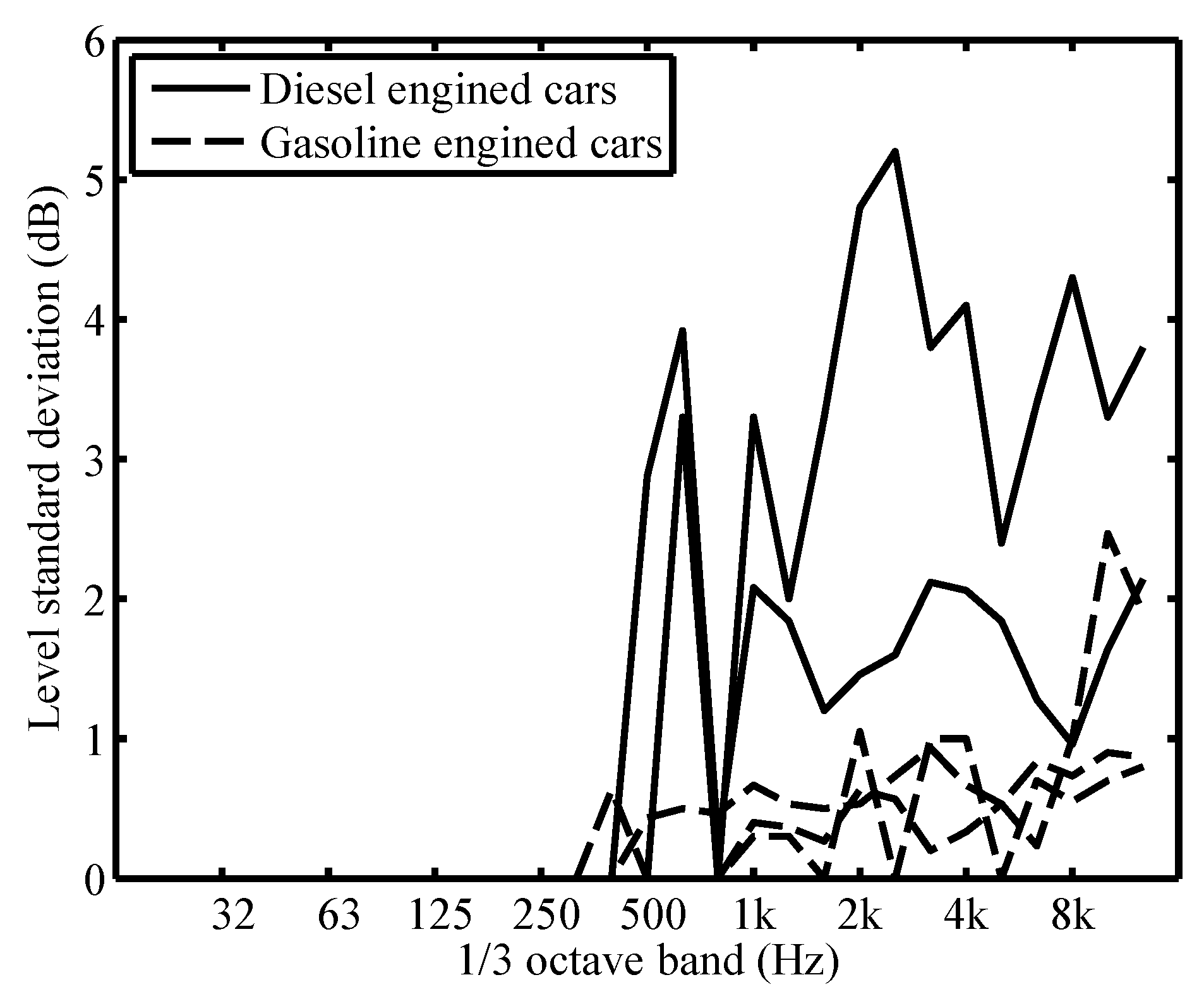
3.2.3. Noise Analysis

The noise levels and their short-term level fluctuations are obtained by a series of filtering operations. Starting with the resampled signal, in a first attempt, the engine orders are suppressed using cascaded notch filters. These filters are designed analogously to the engine order filter bank from the previous section, except that instead of bandpass filters, band-stop filters are generated (see Figure 12). Figure 15 shows two power spectral densities, which illustrate the effect of the order suppression filter. After this operation, the signal is split into sub-bands for further analysis. The signal is therefore decomposed into 1/3 octave bands using a 1/3 octave band filter bank. Each of the $N_b$ filters yields a signal $q_i\left(t\right)$.

Figure 15. Power spectral densities illustrating the effect of the order suppression filter, which is applied to a recording of an inline, four-cylinder engine idling at 4000 rpm.

Figure 15. Power spectral densities illustrating the effect of the order suppression filter, which is applied to a recording of an inline, four-cylinder engine idling at 4000 rpm.

From $q_i\left(t\right)$, the noise levels, $L_{\mathrm{eq},\mathrm{prop},\mathrm{noise},i}$ in Equation (19), are calculated as Leqs. Moreover, from $q_i\left(t\right)$, using a moving average filter, smoothed level-time curves:

$$L_{q,i}\left(t\right)=10·log\left(\frac{1}{K}{\int }_0^K\frac{q_i^2(t+\tau )}{p_0^2}d\tau \right)$$

(42)

are calculated using a window length of $K=4$ ms. Subsequently, from $L_{q,i}$, the mean value is subtracted to obtain a DC-free level fluctuation signal:

$${\Psi }_{q,i}\left(t\right)=L_{q,i}\left(t\right)-\overline{L_{q,i}\left(t\right)}.$$

(43)

Figure 16a exemplifies such a fluctuation signal for the 2.5-kHz band recorded at the front of a diesel engine car. The periodic structure is clearly visible. Following [6], the autocorrelation function (ACF) is used to estimate the standard deviations ${\sigma }_i$ (used in Equation (19)) of the level fluctuations with period $1/F_{\mathrm{ign}}$ by:

$${\sigma }_i^2={\mathrm{ACF}}_{{\Psi }_{q,i}}(1/F_{\mathrm{ign}}).$$

(44)

Figure 16b shows the square root of the ACF of the level fluctuation signal depicted in Figure 16a. Clear peaks can be observed at lag zero and multiples of the ignition period of 34 ms. The standard deviation σ amounts to about 5 dB. The fact that a higher peak appears at the double ignition period, at 68 ms, indicates that the signal contains an additional level modulation with a modulation frequency equal to the half ignition frequency. This can also be observed in Figure 16a in which every second peak is about 5 dB higher than the previous one.

Figure 17 shows measured spectra of the standard deviations ${\sigma }_i$. The measurements were performed in front of five cars idling at low engine speeds. It can be seen that diesel cars feature higher values compared to gasoline engine cars. This finding corresponds to the increased rattling sound noticed in the field.

Figure 16. Level fluctuation signal (a) of the 2.5-kHz 1/3 octave band and its square root of the autocorrelation function (b) from a recording taken at the front of an idling four-cylinder diesel engine at 870 rpm, corresponding to an ignition period of 34 ms. The right plot indicates that for this band, the level standard deviation, σ, amounts to about 5 dB.

Figure 16. Level fluctuation signal (a) of the 2.5-kHz 1/3 octave band and its square root of the autocorrelation function (b) from a recording taken at the front of an idling four-cylinder diesel engine at 870 rpm, corresponding to an ignition period of 34 ms. The right plot indicates that for this band, the level standard deviation, σ, amounts to about 5 dB.

Figure 17. Level fluctuation standard deviations, σ, in 1/3 octave bands measured at the front of two diesel engine and three gasoline engine cars idling at 900 rpm.

Figure 17. Level fluctuation standard deviations, σ, in 1/3 octave bands measured at the front of two diesel engine and three gasoline engine cars idling at 900 rpm.

3.2.4. Background Noise Corrections

On the test rig, the main background noise sources were the tire noise, the airstream fan, the room ventilation and the dynamometer itself. Firstly, to confine the tire noise, the measurements were performed at low vehicle speeds, i.e., low gears. Secondly, during the measurements, the airstream fan (depicted in Figure 8) was briefly switched off for periods of about 10 s. However, the dropping tonal components of the fan still strongly interfered with the propulsion noise of the car (see Figure 18). Therefore, several shifted analysis time windows were deployed, and the minimal levels and the maximum level standard deviations, σ, across these windows were exploited. Thirdly, background noise measurements with a switched off engine at different vehicle speeds were performed. For each ordinary measurement, the corresponding background noise was identically analyzed and used for level corrections.

Figure 18. Normalized spectrogram of a microphone position in front of a Ford Focus 1.8i at 4000 rpm and full load on the dynamometer. The dropping tonal component around 100 Hz stems from the briefly switched off airstream fan of the lab.

Figure 18. Normalized spectrogram of a microphone position in front of a Ford Focus 1.8i at 4000 rpm and full load on the dynamometer. The dropping tonal component around 100 Hz stems from the briefly switched off airstream fan of the lab.

3.2.5. Backpropagation

As the interface to the propagation model, the emission signals are defined at a (virtual) reference distance of $r_0=1$ meter from the source position. For the measured levels $L_{\mathrm{lab}}$, the following inverse sound propagation model is used:

$$L_{\mathrm{Em},1\mathrm{m}}=L_{\mathrm{lab}}+20log\left(\frac{r_{\mathrm{Ac}}}{r_0}\right)+A_{\mathrm{room}}+A_{\mathrm{gr}}$$

(45)

with the ground effect $A_{\mathrm{gr}}=-6$ dB, as all microphones were mounted on the ground. For the microphones placed close to the room edge (emission angles $\phi ={60}^{\circ }$ and 120${}^{\circ }$), the room correction $A_{\mathrm{room}}$ was set to $-6$ dB for frequency bands below 1 kHz and to $-3$ dB otherwise. As for the microphones placed in front and at the back of the car, the distance to the closest wall was about three meters; $A_{\mathrm{room}}$ was set to 0 dB for these signals. $r_{\mathrm{Ac}}$ is the distance to the acoustical center, which, by assuming geometrical spreading of a point source, is obtained by simultaneous free field measurements at two points at distances r and $r^{\prime }$ $(r^{\prime }>r)$ with:

$$r_{\mathrm{Ac}}=\frac{r^{\prime }-r}{1-{10}^{\left(L_{\mathrm{ff},r^{\prime }}-L_{\mathrm{ff},r}\right)/20}}$$

(46)

Parameter $r_{\mathrm{Ac}}$ is evaluated separately for each emission angle, engine speed and frequency band (or engine order, respectively).

4. Conclusions

In the proposed auralization model, emission sounds of accelerating passenger cars are artificially generated based on spectral modeling synthesis. Whereas the sound of tires is synthesized as stationary noise, which is time-dependently shaped in third octave bands, the realistic synthesis of sounds of propulsion requires more subtlety.

It is synthesized as the superposition of a noise component and tones. Frequency-dependent periodic short-term modulations are applied to the noise component in order to create a rattling sound eliciting a roughness sensation. The tones are related to the engine orders. It was found that a large number of engine orders are needed (50...100) to convincingly represent different engine speeds and loads. Moreover auralizations revealed that the order phases have to be included as synthesizer parameters. In conclusion, the presented emission synthesizer gives complete control over the signal characteristics, but is computationally much more demanding than a synthesizer based on granular synthesis [5] with limited flexibility. However, a hybrid approach could profit from both advantages, i.e., by pre-creating relevant signal grains using spectral modeling synthesis and usage for granular synthesis in real-time applications.

Analysis of the propagation filtering algorithms yielded two main insights. Aliasing, arising from the simulation of the Doppler effect, can be reduced by incorporating a band-limited resampling strategy, such as the windowed sinc interpolation. Furthermore, due to the low source height, a significantly higher number of filter taps is needed to correctly simulate the ground effect in relevant situations, as compared to elevated sources, such as airplanes or wind turbines [46].

We conclude that with the presented synthesizer structure, audio signals from vehicle pass-bys can be represented in a compact and elegant manner. To give the reader an impression of the subjective quality of the proposed model, auralizations of two examples are published as supplementary data (see the videos in the Supplementary File and Section 2.3 for details).

References

1. Kleiner, M.; Dalenbäck, B.I.; Svensson, P. Auralization—An Overview. J. Audio Eng. Soc. 1993, 41, 861–875. [Google Scholar]
2. Vorländer, M. Auralization: Fundamentals of Acoustics, Modelling, Simulation, Algorithms and Acoustic Virtual Reality; Springer: Berlin, Germany, 2008. [Google Scholar]
3. Savioja, L.; Svensson, U. Overview of geometrical room acoustic modeling techniques. J. Acoust. Soc. Am. 2015, 138, 708–730. [Google Scholar] [CrossRef] [PubMed]
4. Klemenz, M. Sound Synthesis of Starting Electric Railbound Vehicles and the Influence of Consonance on Sound Quality. Acta Acust. United Acust. 2005, 91, 779–788. [Google Scholar]
5. Jagla, J.; Maillard, J.; Martin, N. Sample-based engine noise synthesis using an enhanced pitch-synchronous overlap-and-add method. J. Acoust. Soc. Am. 2012, 132, 3098–3108. [Google Scholar] [CrossRef] [PubMed]
6. Pieren, R.; Heutschi, K.; Müller, M.; Manyoky, M.; Eggenschwiler, K. Auralization of Wind Turbine Noise: Emission Synthesis. Acta Acust. United Acust. 2014, 100, 25–33. [Google Scholar] [CrossRef]
7. Arntzen, M.; Simons, D. Modeling and synthesis of aircraft flyover noise. Appl. Acoust. 2014, 84, 99–106. [Google Scholar] [CrossRef]
8. Sahai, A.; Wefers, F.; Pick, P.; Stumpf, E.; Vorländer, M.; Kuhlen, T. Interactive simulation of aircraft noise in aural and visual virtual environments. Appl. Acoust. 2016, 101, 24–38. [Google Scholar] [CrossRef]
9. Rizzi, S.; Sullivan, B.; Sondridge, C. A three-dimensional virtual simulator for aircraft flyover presentation. In Proceedings of the 2003 International Conference on Auditory Display, Boston, MA, USA, 6–9 July 2003; pp. 87–90.
10. Rietdijk, F.; Heutschi, K.; Zellmann, C. Determining an empirical emission model for the auralization of jet aircraft. In Proceedings of the 10th European Conference on Noise Control, Maastricht, The Netherlands, 31 May–3 June 2015; pp. 781–784.
11. Manyoky, M.; Hayek Wissen, U.; Klein, T.; Pieren, R.; Heutschi, K.; Grêt-Regamey, A. Concept for collaborative design of wind farms facilitated by an interactive GIS-based visual-acoustic 3D simulation. In Proceedings of the Digital Landscape Architecture, Bernburg, Germany, 31 May 2012; pp. 297–306.
12. Manyoky, M.; Hayek Wissen, U.; Heutschi, K.; Pieren, R.; Grêt-Regamey, A. Developing a GIS-Based Visual-Acoustic 3D Simulation for Wind Farm Assessment. ISPRS Int. J. Geo-Inf. 2014, 3, 29–48. [Google Scholar]
13. Forssén, J.; Kaczmarek, T.; Alvarsson, J.; Lundén, P.; Nilsson, M.E. Auralization of traffic noise within the LISTEN project—Preliminary results for passenger car pass-by. In Proceedings of the Eighth European Conference on Noise Control, Edinburgh, UK, 26–28 October 2009.
14. Peplow, A.; Forssén, J.; Lundén, P.; Nilsson, M.E. Exterior Auralization of Traffic Noise within the LISTEN project. In Proceedings of the European Conference on Acoustics (Forum Acusticum 2011), Aalborg, Denmark, 27 June–1 July 2011; pp. 665–669.
15. Maillard, J.; Jagla, J. Real Time Auralization of Non-Stationary Traffic Noise—Quantitative and Perceptual Validation in an Urban Street. In Proceedings of the AIA-DAGA Conference on Acoustics, Merano, Italy, 18–21 March 2013.
16. McDonald, P.; Rice, H.; Dobbyn, S. Auralisation and Dissemination of Noise Map Data Using Virtual Audio. In Proceedings of the Eighth European Conference on Noise Control, Edinburgh, UK, 26–28 October 2009.
17. Fiebig, A.; Genuit, K. Development of a synthesis tool for soundscape design. In Proceedings of the Eighth European Conference on Noise Control, Edinburgh, UK, 26–28 October 2009.
18. Heutschi, K. SonRoad: New Swiss Road Traffic Noise Model. Acta Acust. United Acust. 2004, 90, 548–554. [Google Scholar]
19. Havelock, D.; Kuwano, S.; Vorländer, M. Handbook of Signal Processing in Acoustics; Springer: New York, NY, USA, 2008. [Google Scholar]
20. Pieren, R.; Bütler, T.; Heutschi, K. Auralisation of accelerating passenger cars. In Proceedings of the 10th European Conference on Noise Control, Maastricht, The Netherlands, 31 May–3 June 2015; pp. 757–762.
21. Jonasson, H.G. Acoustical Source Modelling of Road Vehicles. Acta Acust. United Acust. 2007, 93, 173–184. [Google Scholar]
22. Sandberg, U.; Ejsmont, J. Tyre/Road Noise Reference Book; INFORMEX, Harg: Kisa, Sweden, 2002. [Google Scholar]
23. Zeller, P. Handbuch Fahrzeugakustik—Grundlagen, Auslegung, Berechnung, Versuch, 2nd ed.; Vieweg Teubner Verlag: Wiesbaden, Geramny, 2012. [Google Scholar]
24. United Nations. UN/ECE Regulation No. 117: Uniform Provisions Concerning the Approval of Tyres with Regard to Rolling Sound Emissions and/or to Adhesion on Wet Surfaces and/or to Rolling Resistance. Off. J. Eur. Union 2011, 54, 3–63. [Google Scholar]
25. International Organization of Standardization. ISO 11819-1: Acoustics—Measurement of the Influence of Road Surfaces on Traffic Noise—Part 1: Statistical Pass-By Method; ISO: Geneva, Switzerland, 1997. [Google Scholar]
26. Schutte, J.; Wijnant, Y.; de Boer, A. The Influence of the Horn Effect in Tyre/Road Noise. Acta Acust. United Acust. 2015, 101, 690–700. [Google Scholar] [CrossRef]
27. European Commission. Commission Directive (EU) 2015/996 of 19 May 2015 establishing common noise assessment methods according to Directive 2002/49/EC of the European Parliament and of the Council. Off. J. Eur. Union 2015, 58, 1–823. [Google Scholar]
28. Roads, C. The Computer Music Tutorial; MIT Press: Cambridge, MA, USA, 1996. [Google Scholar]
29. Rossing, T. Springer Handbook of Acoustics; Springer: New York, NY, USA, 2007. [Google Scholar]
30. Smith, J., III. Spectral Audio Signal Processing; W3K Publishing: Standford, UK, 2011. [Google Scholar]
31. Serra, X.; Smith, J., III. Spectral Modeling Synthesis: A Sound Analysis/Synthesis System Based on a Deterministic Plus Stochastic Decomposition. Comput. Music J. 1990, 14, 12–24. [Google Scholar] [CrossRef]
32. Serra, X. Musical Sound Modeling with Sinusoids plus Noise. In Musical Signal Processing; Swets & Zeitlinger: Lisse, The Netherlands, 1997. [Google Scholar]
33. International Electrotechnical Commission. IEC 1260:1995: Electroacoustics—Octave-Band and Franctional-Octave-Band Filters; IEC: Geneva, Switzerland, 1995. [Google Scholar]
34. Reif, K. Bosch Automotive Handbook, 8th ed.; Wiley: Chichester, UK, 2011. [Google Scholar]
35. United Nations. UN/ECE/TRANS/WP.29/2014/27: Proposal for a New Global Technical Regulation on the Worldwide harmonized Light vehicles Test Procedure (WLTP); UNECE: Geneva, Switzerland, 2014. [Google Scholar]
36. International Organization of Standardization. ISO 15031-5: Road Vehicles—Communication between Vehicle and External Equipment for Emissions-Related Diagnostics—Part 5: Emissions-related Diagnostic Services; ISO: Geneva, Switzerland, 2015. [Google Scholar]
37. Maekawa, Z. Noise reduction by screens. Appl. Acoust. 1968, 1, 157–173. [Google Scholar] [CrossRef]
38. International Organization of Standardization. ISO 9613-2: Acoustics—Attenuation of Sound during Propagation Outdoors—Part 2: General Method of Calculation; ISO: Geneva, Switzerland, 1996. [Google Scholar]
39. Van Maercke, D.; Defrance, J. Development of an Analytical Model for Outdoor Sound Propagation within the Harmonoise Project. Acta Acust. United Acust. 2007, 93, 201–212. [Google Scholar]
40. Daigle, G.; Embleton, T.; Piercy, J. Propagation of sound in the presence of gradients and turbulence near the ground. J. Acoust. Soc. Am. 1986, 79, 613–627. [Google Scholar] [CrossRef]
41. Hofmann, J.; Heutschi, K. An engineering model for sound pressure in shadow zones based on numerical simulations. Acta Acust. United Acust. 2005, 91, 661–670. [Google Scholar]
42. Wunderli, J.; Pieren, R.; Heutschi, K. The Swiss shooting sound calculation model sonARMS. Noise Control Eng. J. 2012, 90, 224–235. [Google Scholar]
43. Heutschi, K. Calculation of Reflections in an Urban Environment. Acta Acust. United Acust. 2009, 95, 644–652. [Google Scholar] [CrossRef]
44. Wunderli, J. An Extended Model to Predict Reflections from Forests. Acta Acust. United Acust. 2012, 98, 263–278. [Google Scholar] [CrossRef]
45. Pieren, R.; Wunderli, J. A Model to Predict Sound Reflections from Cliffs. Acta Acust. United Acust. 2011, 97, 243–253. [Google Scholar] [CrossRef]
46. Heutschi, K.; Pieren, R.; Müller, M.; Manyoky, M.; Hayek Wissen, U.; Eggenschwiler, K. Auralization of Wind Turbine Noise: Propagation Filtering and Vegetation Noise Synthesis. Acta Acust. United Acust. 2014, 100, 13–24. [Google Scholar] [CrossRef]
47. Lighthill, M. On sound generated aerodynamically. I. General Theory. Proc. R. Soc. Lond. Ser. A 1952, 211, 564–587. [Google Scholar] [CrossRef]
48. Morse, P.; Ingard, K. Theoretical Acoustics; Mc Gray-Hill Book Company: New York, NY, USA, 1968. [Google Scholar]
49. Lighthill, M. The Bakerian Lecture, 1961: Sound Generated Aerodynamically. Proc. R. Soc. Lond. Ser. A 1962, 267, 147–182. [Google Scholar] [CrossRef]
50. Smith, J.; Serafin, S.; Abel, J.; Berners, D. Doppler Simulation and the Leslie. In Proceedings of the 5th International Conference on Digital Audio Effects, Hamburg, Germany, 26–28 September 2002; pp. 932–937.
51. Laakso, T.I.; Välimäki, V.; Karjalainen, M.; Laine, U.K. Splitting the unit delay—Tools for fractional delay filter design. IEEE Signal Process. Mag. 1996, 13, 30–60. [Google Scholar] [CrossRef]
52. Bruneau, M. Fundamentals of Acoustics; ISTE Ltd: London, UK, 2006. [Google Scholar]
53. Delany, M.E.; Bazley, E.N. Acoustical properties of fibrous absorbent materials. Appl. Acoust. 1970, 3, 105–116. [Google Scholar] [CrossRef]
54. International Organization of Standardization. ISO 9613-1: Acoustics—Attenuation of Sound During Propagation Outdoors—Part 1: Calculation of the Absorption of Sound by the Atmosphere; ISO: Geneva, Switzerland, 1993. [Google Scholar]
55. Gerzon, M. Periophony: With-Height Sound Reproduction. J. Audio Eng. Soc. 1973, 21, 2–10. [Google Scholar]
56. Gerzon, M. Ambisonics in Multichannel Broadcasting and Video. J. Audio Eng. Soc. 1985, 33, 859–871. [Google Scholar]
57. Pulkki, V. Virtual Sound Source Positioning Using Vector Base Amplitude Panning. J. Audio Eng. Soc. 1997, 45, 456–466. [Google Scholar]
58. Pulkki, V. Uniform spreading of amplitude panned virtual sources. In Proceedings of the IEEE Workshop on Applications of Signal Processing to Audio and Acoustics, New Paltz, NY, USA, 17–20 October 1999.
59. Ballou, G. Handbook for Sound Engineers, 4th ed.; Elsevier: Amsterdam, The Netherlands, 2008. [Google Scholar]
60. Dickreiter, M.; Dittel, V.; Hoeg, W.; Wöhr, M. Handbuch der Tonstudiotechnik—Band 1, 7th ed.; ARD.ZDF medienakademie: Nürnberg, Geramny, 2008. [Google Scholar]
61. Rabiner, L.; Cheng, M.; Rosenberg, A.; McGonegal, C. A comparative performance study of several pitch detection algorithms. IEEE Trans. Acoust. Speech Signal Process. 1976, 24, 399–418. [Google Scholar] [CrossRef]
62. De la Cuadra, P.; Master, A. Efficient pitch detection techniques for interactive music. In Proceedings of the International Computer Music Conference, Havana, Cuba, 17–23 September 2001; pp. 87–90.
63. Gerhard, D. Pitch Extraction and Fundamental Frequency: History and Current Techniques, Technical Report TR-CS 2003-06; Department of Computer Scinece, University of Regina: Regina, SK, Canada, 2003. [Google Scholar]
64. Dreuw, P.; Deselaers, T.; Rybach, D.; Keysers, D.; Ney, H. Tracking Using Dynamic Programming for Appearance-Based Sign Language Recognition. In Proceedings of the IEEE International Conference on Automatic Face and Gesture Recognition, Southampton, UK, 2–6 April 2006; pp. 293–298.