Flexible Transmission Network Expansion Planning Considering Uncertain Renewable Generation and Load Demand Based on Hybrid Clustering Analysis

Abstract

This paper presents a flexible transmission network expansion planning (TNEP) approach considering uncertainty. A novel hybrid clustering technique, which integrates the graph partitioning method and rough fuzzy clustering, is proposed to cope with uncertain renewable generation and load demand. The proposed clustering method is capable of recognizing the actual cluster distribution of complex datasets and providing high-quality clustering results. By clustering the hourly data for renewable generation and load demand, a multi-scenario model is proposed to consider the corresponding uncertainties in TNEP. Furthermore, due to the peak distribution characteristics of renewable generation and heavy investment in transmission, the traditional TNEP, which caters to rated renewable power output, is usually uneconomic. To improve the economic efficiency, the multi-objective optimization is incorporated into the multi-scenario TNEP model, while the curtailment of renewable generation is considered as one of the optimization objectives. The solution framework applies a modified NSGA-II algorithm to obtain a set of Pareto optimal planning schemes with different levels of investment costs and renewable generation curtailments. Numerical results on the IEEE RTS-24 system demonstrated the robustness and effectiveness of the proposed approach.

1. Introduction

With the rapid development of renewable energy recently, renewable generation will be extensively utilized in the smart grid of the near future to mitigate environmental pollution and promote sustainable development. However, owing to the stochastic volatility and intermittency of renewable energy, the integration of renewable energy sources would possibly exacerbate the uncertainty of power systems, which brings a series of new challenges to transmission network expansion planning (TNEP). Hence, it is necessary to present an economic and robust TNEP method to deal with renewable energy integration in the smart grid.

In the literature, there have been several studies on the TNEP problem under uncertainty by adopting mathematical optimization methods. For instance, [1] employed methods of stochastic programming and probabilistic constraints for generation and transmission expansion planning with consideration of uncertainties in power system operation. In [2], a chance-constrained programming method was proposed to deal with uncertain load and wind power in TNEP. However, the stochastic optimization generally requires the accurate probability density function (PDF) of each uncertain parameter as well as the deterministic form of constraints associated with uncertainties, which are difficult to achieve in practice. Apart from stochastic optimization, robust optimization has also been widely discussed in TNEP. Since robust optimization only requires the lower and upper bounds of uncertain parameters, uncertainties such as load demand, renewable generation, and transmission investment cost [3,4] can be easily considered in TNEP through a robust model. Nevertheless, the robust TNEP method also has the issue of over-conservatism and may lead to uneconomic solutions.

Recently several researchers have employed the multi-scenario method in TNEP, which considers uncertainties by multiple scenarios. The works by [5,6] adopted a scenario-generation method to deal with uncertain generation dispatch. [7] applied the Monte Carlo simulation (MCS) to simulate the uncertainties of outages and load forecasting in the coordinated generation-transmission expansion planning. In addition, the robust TNEP design based on extreme scenarios was adopted by [8,9] to improve the robustness of planning schemes. Nevertheless, the above multi-scenario methods still have limitations, as they tend to generate a large number of scenarios to achieve accurate simulation of uncertainties, which may cause a heavy computational burden.

With the integration of large-scale renewable energy, the penetration level of renewable generation is generally high in the smart grid. Under such circumstances, the traditional TNEP methods, which cater for rated renewable power output, may lead to low utilization rates of transmission lines and poor economic efficiency [10]. In addition, since the power output of spatially dispersed renewable power plants tends to be strongly correlated in many geographical regions [11], the assumption that each renewable power plant is independent is no longer applicable. Recently several studies have emphasized the necessity of considering spatio-temporal correlation among renewable energy sources in various fields of the power system, such as wind power forecasting [11], power market [12], etc. Accordingly, the spatial correlation among different renewable power plants also needs to be considered in TNEP to improve the simulation accuracy of uncertain renewable generation.

Although much research has been devoted to the TNEP problem under uncertainty, few studies have investigated the impact of the peak distribution characteristics of renewable generation on the economic efficiency of TNEP. Hence, the purpose of this paper is to provide economic and flexible planning schemes considering uncertainty. A novel scenario-generation method based on clustering analysis is proposed first to handle uncertain factors. In contrast with the scenario-generation methods discussed above, the proposed method only requires the raw information of uncertain factors, and is capable of controlling the number of scenarios to an acceptable range. More importantly, it can spontaneously take into account the correlation among uncertain factors when generating typical scenarios, thus improving the accuracy of uncertainty simulation. Furthermore, on the basis of the typical scenarios, this paper presents a multi-scenario, multi-objective TNEP model with consideration of uncertain renewable generation and load demand. In order to achieve the balance between economic efficiency and robustness of TNEP, the curtailment of renewable generation is considered as one of the optimization objectives. A modified NSGA-II algorithm is then employed to obtain a set of Pareto optimal planning schemes with different levels of investment costs and renewable generation curtailments. In consequence, decision makers are allowed to make an effective choice according to the Pareto optimal front. For validation, the proposed TNEP method is tested on the modified IEEE RTS-24 system. The numerical results show that the proposed method can provide planning schemes superior to those from conventional TNEP methods.

2. Uncertainty Processing Based on Clustering Technique

It has been discussed above that an effective set of scenarios can be employed to guide the TNEP design of a smart grid under uncertainty. Obviously, the accuracy of uncertainty simulation has a direct effect on the validity of planning results, and the number of scenarios is also related to the computational efficiency of TNEP problem solving. When dealing with large uncertainties, the conventional scenario-generation methods can hardly guarantee simulation accuracy while controlling the scenarios’ number within an acceptable range. In addition, the difficulty of uncertainty simulation in the smart grid is also significantly increased due to the large-scale utilization of renewable energy. Therefore, an effective scenario-generation method is of great importance.

Since it is one of the major characteristics of a smart grid to have massive amounts of data collected from various measuring devices [13], this paper proposes a novel scenario-generation method based on clustering analysis to cope with the uncertainty in the form of large datasets. As one of the most commonly used data mining techniques, clustering analysis has been proven to be effective to recognize the accurate distribution characteristics of large datasets [14]. In this paper, the power dataset to be clustered consists of the raw data for each uncertain factor, such as hourly data of wind power, photovoltaic power, load demand, etc. Through the clustering analysis, the power dataset can be clustered into several clusters where data samples belonging to the same cluster have similar values of renewable power output and load demand. This means that each cluster can represent a typical combination of renewable power output and load demand, while the correlation among the uncertain factors is considered intuitively. Therefore, a scenario set, which contains the typical combinations of renewable power output and load demand, can be selected from the clusters by data sampling.

This paper proposes a novel hybrid clustering method that thoroughly investigates the inherent characteristics of the TNEP problem. Moreover, an effective strategy for scenario selection is applied to ensure the typicality of the selected scenario set. The specific procedures are described in the following subsections.

2.1. Identification of the Number of Typical Combinations of Renewable Power Output and Load Demand

For the power dataset, each data sample represents a deterministic combination of renewable power output and load demand, while an effective scenario set should contain all the typical combinations. Since data samples belonging to the same cluster have similar values of renewable power output and load demand, each cluster can be considered as a specific data subset representing a typical combination. Thus the optimal cluster number for a power dataset, which corresponds to the number of typical combinations, needs to be identified first.

This section employs an iterative graph partitioning method to obtain the optimal cluster number [15]. This method approaches the problem with two kinds of matrix forms: the observation matrix and the judgement matrix. Suppose the dataset x with n data samples has been already clustered into h clusters, then an n×n observation matrix M^O is given by:

$$M_{ij}^O=\{\begin{array}{l}1x_i,x_j\in Cluster\mathsf{\eta }\\ 0x_i,x_j\notin Cluster\mathsf{\eta }\end{array}(\mathsf{\eta }\in [1,h])$$

(1)

The observation matrix M^O represents the clustering relationships among all the data samples under a defined cluster number. Obviously, a single observation matrix can hardly reveal the accurate clustering distribution of a complex dataset, especially when the optimal cluster number is unknown. Thus it is essential to compute the observation matrices with different cluster numbers to obtain more clustering information. Suppose there is an observation matrix set with the total number c of clusters ranging from 2 to k, the judgement matrix M^J is defined as follows to extract the key information:

$$M^J={\displaystyle \sum _{c=2}^k{M}_c^O}$$

(2)

where $M_c^O$ is the observation matrix with the cluster number set to c. It can be observed that the judgement matrix M^J integrates the clustering relationships among data samples under different cluster numbers. The value of each matrix element indicates the similarity degree between the corresponding data samples; for example, a large value of $M_{\mathit{ij}}^J$ means a high similarity degree between x_i and x_j, and in that case there will be a high probability that x_i and x_j are grouped into the same cluster.

On the basis of the above two kinds of matrix forms, the steps of the identification method are given in brief below [15]:

(a)

Employ the partitioning clustering algorithm to cluster the power dataset iteratively with the cluster number ranging from 2 to k, then obtain the observation matrix set according to Equation (1).

(b)

Compute the judgement matrix M^J as the sum of the obtained observation matrix set.

(c)

On the basis of Breadth-First Search (BFS) algorithm, record the number of independent connected sub-matrices in M^J. The recorded number represents the total number of clusters in the current iteration.

(d)

Update the judgement matrix M^J by decreasing the value of each non-zero element as follows:

$$M_{ij}^J=\{\begin{array}{l}{M}_{ij}^J-1if{M}_{ij}^J\ge 1\\ 0otherwise\end{array}$$

(3)

(e)

If all elements of the updated judgement matrix M^J become zero, then go to the next step. Otherwise, go to step (c).

(f)

Analyze the recorded number of sub-matrices in all iterations. The number with the maximum stability degree is viewed as the optimal cluster number.

In step (f), the stability degree of a given sub-matrix number c refers to the consecutive occurrence number of c in all iterations. The number with the maximum stability degree means that under this number, the connections of the data samples within the sub-matrices (clusters) are the strongest and hardest to break [15].

It should be noted that the partitioning clustering algorithm is employed as a fast clustering technique to accelerate the iterative clustering process in step (a). However, its clustering performance is not sufficiently stable when the cluster number is large. To solve this issue, the above identification process is repeated s_n times in this paper. Based on s_n times calculation, the stability degree of each sub-matrix number can be estimated accurately and the optimal cluster number can be determined through further statistical analysis.

2.2. Rough Fuzzy Clustering Analysis of Power Dataset

Since the uncertainty level in different TNEP cases may vary significantly, it is important to adopt a flexible clustering method to ensure good clustering performance under various datasets.

Traditional clustering methods, such as hard clustering, in which the membership degree of each data sample should only be 0 or 1, are not suitable for TNEP because the power data is inherently continuous. Although soft clustering can deal with continuous data by fuzzy membership degree, it also has the shortcoming of producing overlapped clusters.

Considering the intrinsic characteristics of power dataset, this paper adopts a rough-fuzzy clustering method, which is based on minimizing the following objective function [16]:

$$f={\displaystyle \sum _{j=1}^h{\displaystyle \sum _{i=1}^n{u}_{ij}^{q}d{(x_i,{\mathsf{\lambda }}_j)}^q}}$$

(4)

where h is the cluster number; n is the sample number of the power dataset; u_ij is the membership degree of data sample x_i to cluster j; q is the fuzzifier parameter set as 2; and d(x_i,λ_j) is the Euclidean distance between x_i and cluster center λ_j, which represents the similarity degree between the power values of x_i and λ_j.

Unlike traditional clustering, the rough-fuzzy membership degree is applied in the adopted method to guide the clustering analysis. The corresponding membership degree matrix u is obtained by the following steps [17]:

(a)

Calculate the n × h dissimilarity matrix F by measuring the Euclidean distance between each data sample and each cluster center.

(b)

Sort the elements of the matrix F by row in ascending order and obtain a new dissimilarity matrix F′. Then modify the sorted matrix F′ as follows [17]:

$$F\prime (x_i,{\mathsf{\lambda }}_j)=+\infty if\frac{F\prime (x_i,{\mathsf{\lambda }}_j)}{F\prime (x_i,{\mathsf{\lambda }}_1)}>1.2(i\in [1,n],j\in [2,h])$$

(5)

(c)

Convert the modified matrix F’ into the matrix F with the original order. Then calculate the membership degree matrix u by:

$$u_{ij}=F{(x_i,{\mathsf{\lambda }}_j)}^{-\frac{2}{q-1}}/{\displaystyle \sum _{k=1}^{h}F{(x_i,{\mathsf{\lambda }}_k)}^{-\frac{2}{q-1}}}$$

(6)

As shown in Equations (5) and (6), the 0–1 membership degree is employed if the data sample is closed to the cluster center; otherwise the fuzzy membership degree is employed. On the basis of this mixed membership degree, the rough-fuzzy clustering method integrates the advantages of hard clustering and soft clustering [16].

The value of cluster center λ_j is updated with the changes of membership degree matrix u:

$${\mathsf{\lambda }}_j={\displaystyle \sum _{i=1}^n{u}_{ij}^q{x}_i}/{\displaystyle \sum _{i=1}^n{u}_{ij}^q}(i\in [1,n],j\in [1,h])$$

(7)

Through the above analysis, the mathematical formulation of the rough-fuzzy clustering analysis is represented by Equations (4)–(7). A differential evolution algorithm is adopted to solve the above optimization problem; the detailed solving process can be found in [18].

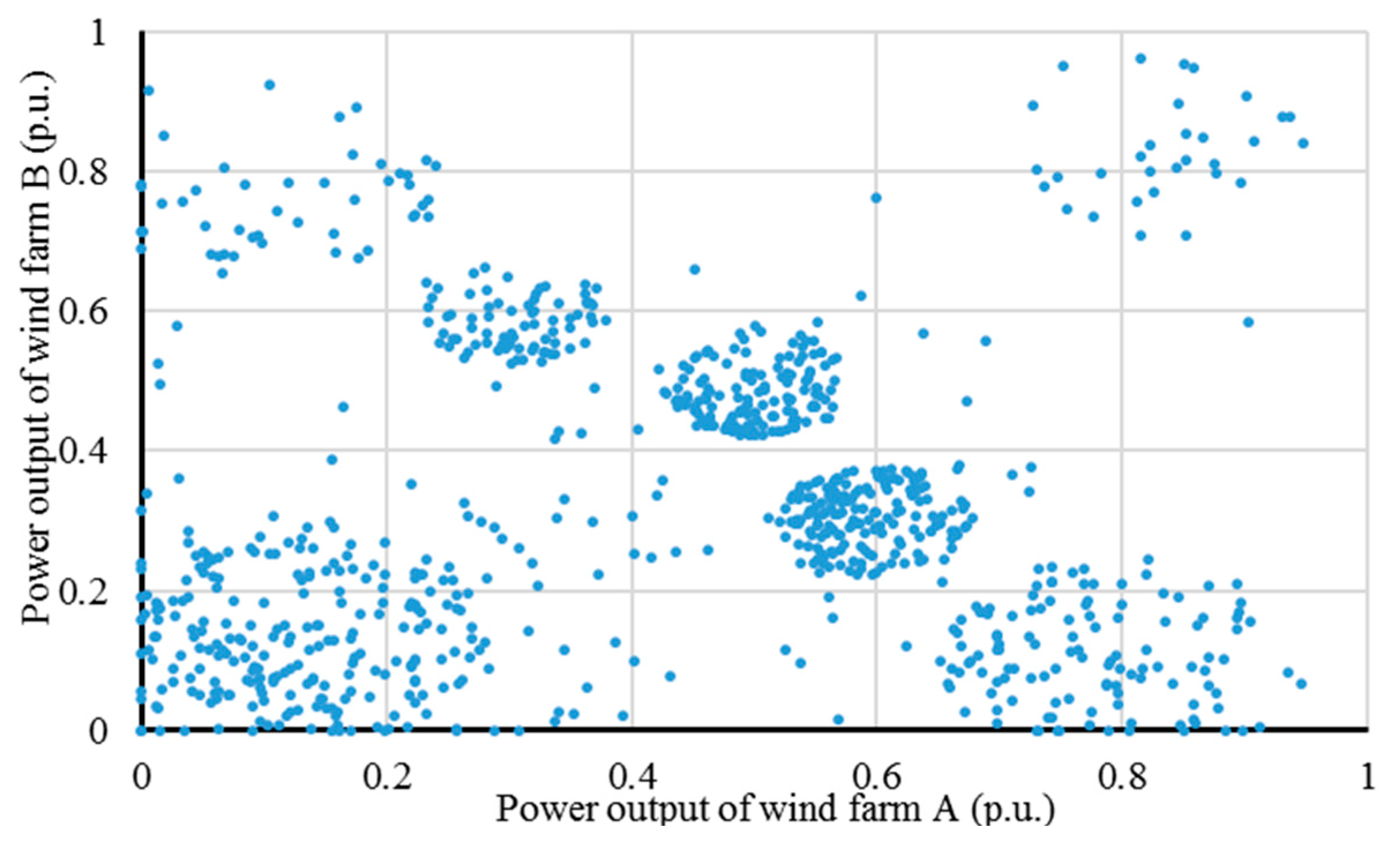
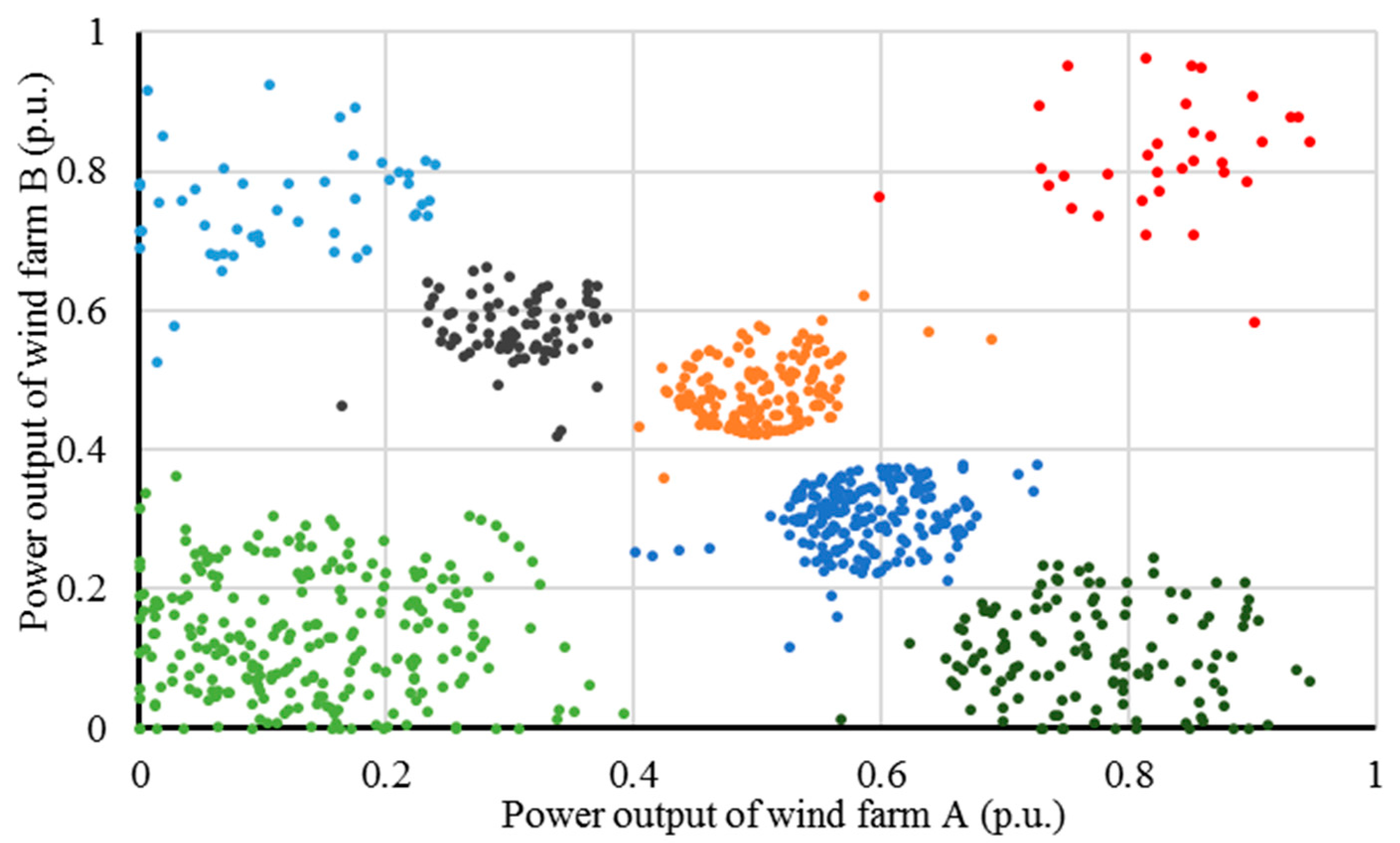
2.3. Validation of the Hybrid Clustering Method with a Wind Power Dataset

A typical wind power dataset, which is derived from two wind farms in the EWITS study [19], is employed to validate the proposed clustering method. Figure 1 gives its scatter diagram:

Figure 1. Scatter distribution of the wind power dataset.

Figure 1. Scatter distribution of the wind power dataset.

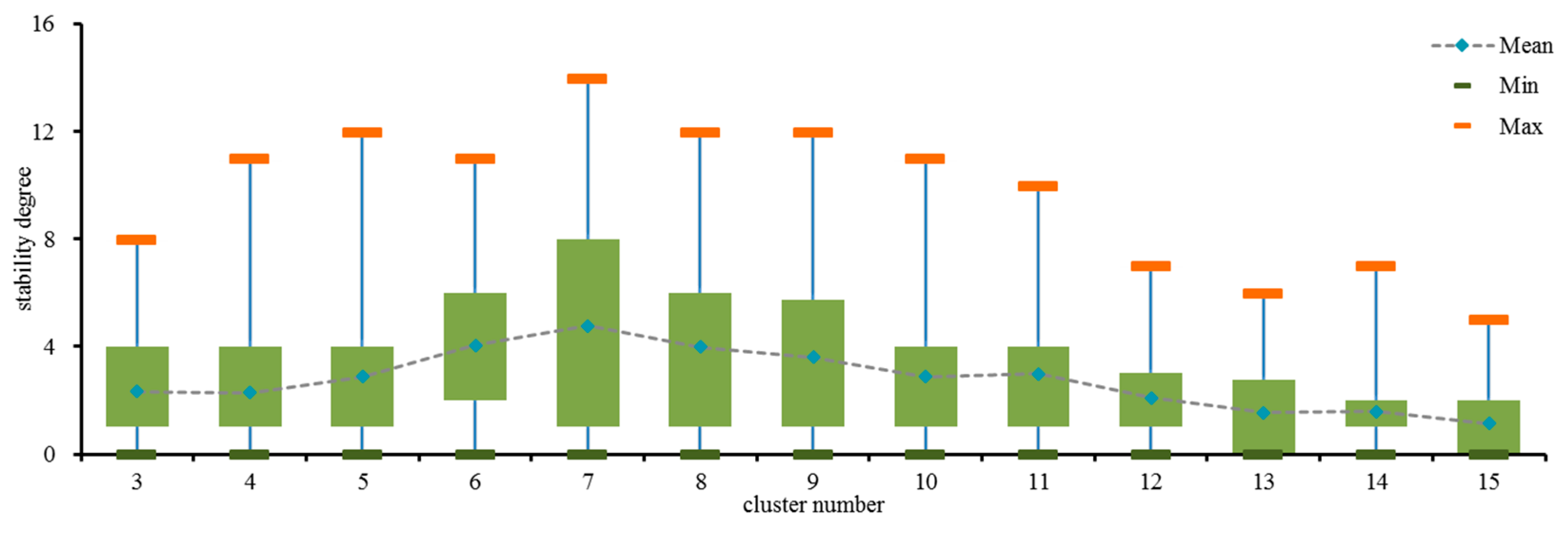
The identification of cluster number is implemented first. Here the parameter s_n is set as 40 by experiments with test databases [20]. Through analyzing the estimated stability degree of each cluster number in 40 trials, statistical results with the cluster number varying from 3 to 15 are illustrated in Figure 2.

According to Figure 2, the cluster number 7, which has the maximum stability degree, is determined as the optimal cluster number. Then the power dataset is clustered into seven clusters as depicted in Figure 3. It can be seen that the clustering result accurately recognizes seven typical combinations of wind power output of the two wind farms. Moreover, there are no overlapping areas among different clusters, showing that the cluster divisions are totally obvious. Hence, the effectiveness of the hybrid clustering method is verified.

Figure 2. Stability degree boxplot for cluster number analysis.

Figure 2. Stability degree boxplot for cluster number analysis.

Figure 3. Clustering result of wind power dataset.

Figure 3. Clustering result of wind power dataset.

2.4. Selection Strategy for Power System Planning Scenarios from Clustering Result

In order to ensure that the selected scenarios can contain sufficient information on the whole power dataset, as well as control the scenarios’ number to an acceptable range, this paper proposes an effective data sampling strategy as follows:

(a)

On the basis of clustering results, calculate the radius of each cluster as follows:

$$r_i=\frac{{\displaystyle \sum _{k=1}^{n_i}d(x_k,{\mathsf{\lambda }}_i)}}{n_i}$$

(8)

where r_i is the radius of the ith cluster; n_i is the data sample number of cluster i; and x_k is the data sample belonging to cluster i.

(b)

Set t_min as the minimum sampling number of a single cluster, then determine the sampling number of each cluster by:

$$t_i=\lfloor t_{\min }\frac{r_i}{r_{\min }}\rfloor$$

(9)

where t_i is the sampling number of cluster i and symbol “⎿⏌” is the rounded-down value of a quantity. It can be inferred that a large sampling number will be applied to the cluster with a large radius. This means that the cluster having the larger distribution range will be sampled more times, thus fully extracting the corresponding data information.

(c)

According to the calculated sampling number, a total of Σt_i data samples are sampled at random to generate the typical scenario set. For each scenario, the corresponding occurrence probability is given by:

$${\alpha }_k=\frac{n_i}{t_i{\displaystyle {\sum }_{j=1}^h{n}_j}}ifscenariok\in clusteri$$

(10)

where α_k is the occurrence probability of scenario k; h is the cluster number.

(d)

Examine the accuracy of the generated typical scenario set by calculating the correlation coefficient between the data distribution represented by the typical scenario set and the whole power dataset.

(e)

Repeat steps (c)–(d) s_m times. Based on s_m times calculation, the scenario set with the largest correlation coefficient is determined to be the optimal scenario set and is employed in the subsequent TNEP model.

3. Improved Model of TNEP with Uncertain Renewable Generation and Load Demand

3.1. Classical Multi-Scenario TNEP Model

A scenario set that contains all the typical combinations of renewable power output and load demand is generated through the previous clustering method. Hence, the planning objective of TNEP under uncertainty can be simplified to find the most economical planning scheme that satisfies all typical scenarios.

By incorporating the typical scenario set, the classical multi-scenario TNEP model is formulated by [6,8]:

$$minw={\displaystyle \sum _{ij\in \mathsf{\Omega }}{c}_{ij}{n}_{ij}}+\mathsf{\beta }{\displaystyle \sum _{k\in \mathsf{\Phi }}{\displaystyle \sum _{i\in \mathsf{\Psi }}(l_i^k+r_i^k)}}$$

(11)

subject to

$$S\times f^k+g_C^k+g_R^k+l^k=d^k+r^k$$

(12)

$$f_{ij}^k-{\gamma }_{ij}(n_{ij}^0+n_{ij})({\theta }_i^k-{\theta }_j^k)=0$$

(13)

$$\left|f_{ij}^k\right|\le (n_{ij}^0+n_{ij})\overline{f_{ij}}$$

(14)

$$0\le g_C\le \overline{g_C}$$

(15)

$$0\le r^k\le g_R^k$$

(16)

$$0\le l^k\le d^k$$

(17)

$$0\le n_{ij}\le \overline{n_{ij}},n_{ij}\text{ is integer}$$

(18)

where

cij	Cost of line that added to right-of-way i-j
$n_{ij}^0$	Number of lines in service on right-of-way i-j
nij	Number of lines in planning on right-of-way i-j
Ψ	Set of buses
Ω	Set of candidate right-of-ways
Φ	Set of typical scenarios
β	Penalty factor
γij	Susceptance of right-of-way i-j
θ	Voltage angle at node i
f	Vector of active power flow
gC	Vector of conventional generation
gR	Vector of renewable generation
S	Branch-node incidence matrix
l	Vector of curtailed load
d	Vector of load demand
r	Vector of renewable generation curtailment
$\overline{•}$	Denotes the max value of a quantity
${•}^k$	Denotes the value of a quantity in scenario K

The objective of Equation (11) is to find the minimum cost planning scheme that satisfies the load demand and renewable power consumption in all typical scenarios. It can be observed that a sufficiently large penalty factor β can effectively drive both the load shedding and renewable generation curtailment to zero. Constraint Equation (12) is the nodal power balance equation at each bus. Constraint Equation (13) is the DC power flow balance equation at each right-of-way. Constraints Equations (14)–(17) are operation limits of power system for the active power flow in the lines, the conventional generator output, the renewable generation curtailment, and the load shedding, respectively.

3.2. Multi-Scenario Multi-Objective TNEP Model Considering Distribution Characteristics of Renewable Power Output

The classical multi-scenario TNEP model caters to the rated capacity of renewable power plants under all typical scenarios, thus ensuring full consumption of renewable generation. However, according to previous research [10], the power output of renewable energy, especially wind energy, is relatively low in most scenarios, whereas the high level output seldom occurs. Therefore, the planning scheme, which satisfies the rated renewable power output, may lead to poor economic efficiency due to the huge cost of transmission investment in integrating renewable energy sources.

Taking into account the distribution characteristics of renewable power, an appropriate curtailment of renewable generation is allowed in this paper to save the transmission investment. Obviously, the transmission investment conflicts with the curtailment level of renewable generation. A high investment in TNEP tends to reduce the curtailment of renewable generation, and vice versa. Consequently, a multi-objective TNEP model is proposed to obtain a Pareto optimal set of planning schemes with different levels of investment costs and renewable generation curtailments. According to the classical TNEP model, the proposed multi-scenario multi-objective TNEP model is formulated as follows:

$$\min \{w_1,w_2\}$$

(19)

subject to Equations (12)–(18) and

$$w_1={\displaystyle \sum _{ij\in \mathsf{\Omega }}{c}_{ij}{n}_{ij}}$$

(20)

$$w_2={\displaystyle \sum _{k\in \mathsf{\Phi }}{\displaystyle \sum _{i\in \mathsf{\Psi }}{\alpha }_k{r}_i^k}}+\mathsf{\beta }{\displaystyle \sum _{k\in \mathsf{\Phi }}{\displaystyle \sum _{i\in \mathsf{\Psi }}{l}_i^k}}$$

(21)

It can be seen that the occurrence probability α_k is applied in Equation (21) to compute the expected renewable generation curtailment under all typical scenarios, which is a new objective to be optimized. In addition, the penalty factor β is also employed to avoid the load shedding. By introducing and optimizing two conflicting objectives, decision makers can make a more effective trade-off between transmission investment cost and renewable generation curtailment according to the actual situation of TNEP.

4. The Solution Method Based on Modified NSGA-II

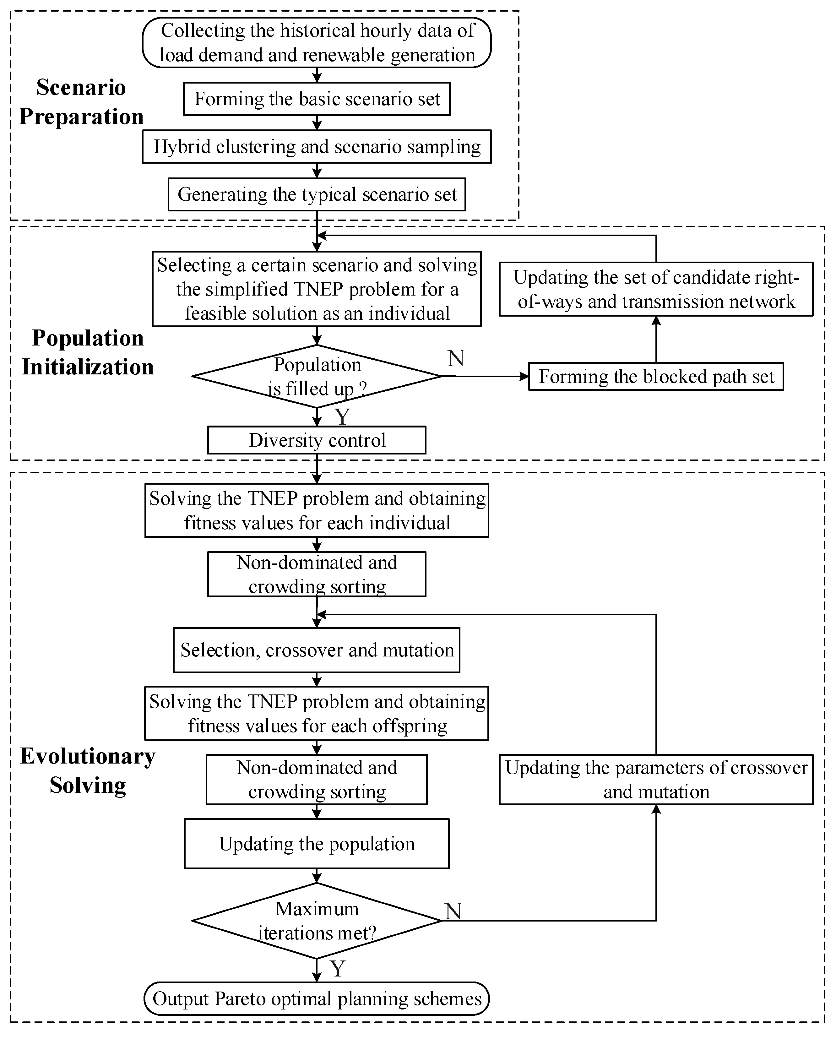
Since the evolutionary algorithm has been proven to be efficient to solve the TNEP problem [21,22], this paper adopted a modified NSGA-II to solve the above multi-objective TNEP problem. Figure 4 shows the solving process of the proposed TNEP model, while the detail of each part is given below.

Figure 4. The solving process of TNEP problem by the modified NSGA-II.

Figure 4. The solving process of TNEP problem by the modified NSGA-II.

4.1. Scenario Preparation for TNEP

In the beginning, the hourly data of each uncertain factor is collected to form the basic scenario set. Then the proposed clustering method is employed to cluster the basic scenario set and to recognize all the typical combinations. Furthermore, a typical scenario set is generated from the clustering results by means of the proposed sampling strategy.

4.2. The Initialization of Population

To speed up the convergence of problem solving, the initial population is generated based on the typical scenario set. For each individual, its initialization procedures are as follows:

(a)

Select a certain scenario with deterministic load demand and renewable generation from the typical scenario set.

(b)

According to the selected scenario, the original TNEP problem is simplified to a single-scenario single-objective problem, in which Equation (21) or Equation (22) is selected alternatively as the optimization objective.

$$w_3={\displaystyle \sum _{ij\in \mathsf{\Omega }}{c}_{ij}{n}_{ij}}+\mathsf{\beta }{\displaystyle \sum _{k\in \mathsf{\Phi }}{\displaystyle \sum _{i\in \mathsf{\Psi }}{l}_i^k}}$$

(22)

(c)

Solve the simplified problem by using software for MILP. The linearization method of Equation (13) can be found in [3]. The obtained planning result is considered as an individual.

It should be noted that the above initialized method may result in similar individuals, which will affect the global search in the subsequent problem solving. Hence, the idea of the “blocked path” is adopted to diversify the initial individuals [6]. After each individual is generated, the right-of-ways where n_ij ≠ 0 are selected to form the blocked path set Γ, which is defined by:

$$i-j\in \{\begin{array}{l}\mathsf{\Gamma },n_{ij}^{new}=rand[0,n_{ij}]ifrand[0,n_{ij}]\ne 0\\ \mathsf{\Omega },n_{ij}=0otherwise\end{array}$$

(23)

where i-j is the right-of-way between nodes i-j; Ω is the set of candidate right-of-ways; rand [0,n_ij] is to generate a random integer within [0, n_ij]. It can be seen that the set of candidate right-of-ways is updated by removing the right-of-ways in the blocked path set. Moreover, for each right-of-way in the blocked path set, $n_{\mathit{ij}}^{\mathit{new}}$ lines are added to the original transmission network. With the updated candidate set and transmission network, the new individuals can be guaranteed to be different from one to another while the initial search area is also expanded.

After all individuals are generated, the diversity check and mutation manipulation are also conducted to ensure that any two individuals are different in at least two right-of-ways.

4.3. Procedures of Evolutionary Solving

(a)

With the planning result determined by each individual, solve the simplified multi-scenario TNEP problem in turn. The optimization results, which include transmission investment cost and curtailed renewable generation, are considered as two fitness values for the corresponding individual.

(b)

For all individuals, carry out the non-dominated and crowding sorting according to the fitness values.

(c)

On the basis of the sorting results, tournament selection, single-point crossover and mutation are implemented to generate offspring. In this paper, the mutation manipulation is to add or remove a line for a selected right-of-way with 50/50 probability [5,6].

(d)

Likewise, solve the simplified TNEP problem for each offspring, and integrate the offspring and parent population for non-dominated and crowding sorting. Then update the population by removing the individuals with the lowest ranking.

(e)

If maximum iterations are met, go to step (f). Otherwise, update the parameters of crossover and mutation as follows, then go to step (c):

$$P_{CR}=0.8-\lceil \frac{i{t}_c}{i{t}_a}\rceil \times 0.1$$

(24)

$$P_{MU}=0.2+\lceil \frac{i{t}_c}{i{t}_a}\rceil \times 0.1,d_{MU}=6-\lceil \frac{i{t}_c}{i{t}_a}\rceil \times 0.1$$

(25)

where P_CR and P_MU are the parameters of crossover probability and mutation probability respectively; it_c is the current number of iterations; it_a is an artificial parameter, which is set to be 20% of the maximum iteration number; symbol “⎾⏋” denotes the rounded-up value of a quantity; and d_MU is the mutation operator, which represents the number of right-of-ways that should mutate in a mutation manipulation.

(f)

Output the planning results from the Pareto optimal front.

According to the idea in [23], this paper proposes an adaptive control strategy for the parameters of crossover and mutation in step (e). With Equations (24) and (25), large values of P_CR and d_MU are employed in the early iterations to diversify the search area and to ensure the global optimization. In later iterations, as the global optimal area is gradually determined, a large value of P_MU is employed while d_MU decreases, which means that a large number of individuals will be mutated and few right-of-ways (d_MU will eventually be decreased to 1) will be changed for each individual. Since the mutation manipulation is only to add or remove a line for each selected right-of-way, a large value of P_MU is employed in later iterations to enhance the local search; this will not have an adverse effect on the optimal solution.

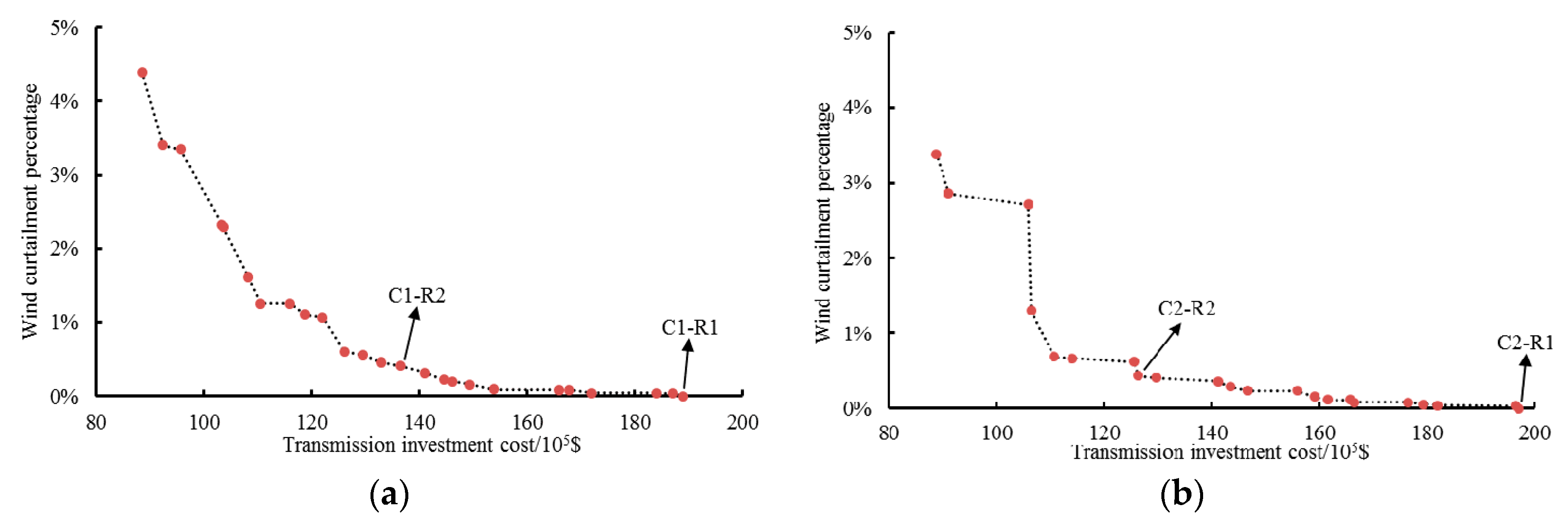
5. Case Study

5.1. Case Description

The proposed TNEP approach is tested on the modified IEEE RTS-24 system; the test system data is available in [24,25]. In this paper, the uncertainties considered in TNEP are load demand and wind generation. The basic scenario set for clustering analysis consists of 8760 hourly data of load demand and wind power output. The hourly load data is simulated by adding a 5% disturbance that follows the normal distribution to the base load data [24]. The hourly wind power data is converted from the actual annual hourly wind speed data, which is derived from the EWITS study [19].

In the modified IEEE RTS-24 system, all the loads are assumed to be 2.8 times of the original values, while all the generation capacities are assumed to be 2.5 times of the original values. Three new buses, Bus-25, Bus-26, and Bus-27, are added, each with a wind capacity of 1000 MW; they can be integrated into the system by the right-of-way 16–25, 7–26, and 1–27. The network topology of the modified IEEE RTS-24 system is shown in Figure 5.

The dashed line in Figure 5 represents the new right-of-ways. A total of 44 right-of-ways are allowed to build new transmission lines, the number of which should be no more than four in each right-of-way.

The parameters are set as follows: the range of cluster number is set to [2,500]; the repetition s_n for cluster number analysis is set at 40, the repetition s_m for scenario sampling is set at 5000; penalty factor β is set as 10⁶ $/MW; the population number is set as 60 based on [5,8]; the maximum number of iterations is set as 1500, which is a relatively large value to guarantee the optimality of the Pareto front.

Figure 5. Network topology of the modified IEEE RTS-24 system.

Figure 5. Network topology of the modified IEEE RTS-24 system.

5.2. Planning Results

The identification of the optimal cluster number is first implemented and the statistical results with the cluster number varying from 3 to 25 are shown in Figure 6.

Figure 6. Stability degree boxplot for cluster number analysis.

Figure 6. Stability degree boxplot for cluster number analysis.

As shown in Figure 6, cluster number 19, which has the maximum stability degree in 40 trials, is determined as the optimal cluster number. Then, with the minimum sampling number t_min set as 3, the basic scenario set is divided into 19 clusters, while a total of 194 scenarios are generated for TNEP.

By solving the proposed TNEP problem, the Pareto optimal front of planning results is obtained. In this paper, only the planning result with a wind curtailment percentage less than 5% is considered as a feasible planning scheme, thus ensuring a certain degree of wind power consumption. Figure 7 shows all feasible planning schemes from the Pareto front. It can be seen that the investment cost in each planning scheme ranges from 91.3 × 10⁵ $ to 165 × 10⁵ $, while the wind curtailment percentage decreases from 4.75% to 0%.

Figure 7. Feasible planning results for IEEE RTS-24 system.

Figure 7. Feasible planning results for IEEE RTS-24 system.

To further investigate the impact of wind power distribution characteristics on TNEP, four feasible planning schemes, which have been marked in Figure 7, are selected for comparison. The detailed information is given in Table 1.

Table 1. Four planning schemes for IEEE RTS-24 system.

Planning Schemes	Cost (×105 $)	Wind Curtailment Percentage	Planning Schemes
R1	165.0	0.00%	n1–2 = 2, n1–5 = 1, n6–10 = 1, n7–8 = 4, n8–9 = 1, n10–12 = 1, n14–16 = 1, n2–8 = 1, n16–25 = 3, n7–26 = 3, n1–27 = 3
R2	145.1	0.15%	n1–2 = 2, n1–5 = 1, n6–10 = 1, n7–8 = 3, n8–9 = 1, n10–12 = 1, n14–16 = 1, n16–25 = 3, n7–26 = 2, n1–27 = 3
R3	123.8	0.40%	n1–2 = 2, n6–10 = 1, n7–8 = 3, n10–12 = 1, n14–16 = 1, n16–25 = 3, n7–26 = 2, n1–27 = 2
R4	108.2	0.82%	n1–2 = 2, n6–10 = 1, n7–8 = 3, n10–12 = 1, n14–16 = 1, n16–25 = 2, n7–26 = 2, n1–27 = 2

Table 1. Four planning schemes for IEEE RTS-24 system.

Planning Schemes	Cost (×105 $)	Wind Curtailment Percentage	Planning Schemes
R1	165.0	0.00%	n1–2 = 2, n1–5 = 1, n6–10 = 1, n7–8 = 4, n8–9 = 1, n10–12 = 1, n14–16 = 1, n2–8 = 1, n16–25 = 3, n7–26 = 3, n1–27 = 3
R2	145.1	0.15%	n1–2 = 2, n1–5 = 1, n6–10 = 1, n7–8 = 3, n8–9 = 1, n10–12 = 1, n14–16 = 1, n16–25 = 3, n7–26 = 2, n1–27 = 3
R3	123.8	0.40%	n1–2 = 2, n6–10 = 1, n7–8 = 3, n10–12 = 1, n14–16 = 1, n16–25 = 3, n7–26 = 2, n1–27 = 2
R4	108.2	0.82%	n1–2 = 2, n6–10 = 1, n7–8 = 3, n10–12 = 1, n14–16 = 1, n16–25 = 2, n7–26 = 2, n1–27 = 2

As shown in Table 1, compared with the most robust planning scheme R1, the investment costs of the other three planning schemes are reduced by 12.06%, 24.97%, and 34.42%, respectively, whereas the wind curtailment percentages are only 0.15%, 0.40%, and 0.82%, respectively, of the expected wind power output. It can be observed that the investment cost of TNEP can be substantially reduced by limiting the wind power output, which only results in an extremely small wind curtailment. As a result, allowing an appropriate renewable curtailment can effectively improve the economic efficiency of TNEP for integrating renewable energy sources.

The above analysis demonstrates that the proposed TNEP method can provide a robust planning scheme and other economic planning schemes simultaneously. Thus decision makers can make an effective trade-off between robustness and economic efficiency and choose the most suitable planning scheme based on actual situations.

5.3. Performance Analysis of the Pareto Optimal Planning Results

To illustrate the effectiveness of the obtained planning results, a total of 30,000 testing scenarios, which are generated by MCS with consideration to wind speed correlation [26], are applied to test the performance of each planning result.

The robustness of planning schemes R1 is verified by estimating the robustness degree with testing scenarios [3,8]. Two robust planning schemes R1-A and R1-B, which are obtained by the genetic algorithm combined with Taguchi’s orthogonal array testing (TOAT) [8] and robust TNEP (RTNEP) [3], respectively, are also evaluated for comparison. Table 2 gives the comparison results of three robust planning schemes.

Table 2. Robustness analysis.

Planning Schemes	Solution	Cost (×105 $)	Robustness Degree
R1	n1–2 = 2, n1–5 = 1, n6–10 = 1, n7–8 = 4, n8–9 = 1, n10–12 = 1, n14–16 = 1, n2–8 = 1, n16–25 = 3, n7–26 = 3, n1–27 = 3	165.0	99.90%
R1-A by TOAT	n1–2 = 2, n1–5 = 1, n2–4 = 1, n6–10 = 1, n7–8 = 4, n8–9 = 1, n8–10 = 1, n2–8 = 1, n16–25 = 3, n7–26 = 3, n1–27 = 3	162.2	99.48%
R1-B by RTNEP	n1–2 = 2, n1–5 = 1, n2–4 = 1, n3–24 = 1, n5–10 = 1, n6–10 = 1, n7–8 = 4, n8–9 = 1, n8–10 = 1, n10–12 = 1, n14–16 = 1, n15–24 = 1, n16–17 = 1, n16–25 = 3, n7–26 = 3, n1–27 = 3	187.4	100%

Table 2. Robustness analysis.

Planning Schemes	Solution	Cost (×105 $)	Robustness Degree
R1	n1–2 = 2, n1–5 = 1, n6–10 = 1, n7–8 = 4, n8–9 = 1, n10–12 = 1, n14–16 = 1, n2–8 = 1, n16–25 = 3, n7–26 = 3, n1–27 = 3	165.0	99.90%
R1-A by TOAT	n1–2 = 2, n1–5 = 1, n2–4 = 1, n6–10 = 1, n7–8 = 4, n8–9 = 1, n8–10 = 1, n2–8 = 1, n16–25 = 3, n7–26 = 3, n1–27 = 3	162.2	99.48%
R1-B by RTNEP	n1–2 = 2, n1–5 = 1, n2–4 = 1, n3–24 = 1, n5–10 = 1, n6–10 = 1, n7–8 = 4, n8–9 = 1, n8–10 = 1, n10–12 = 1, n14–16 = 1, n15–24 = 1, n16–17 = 1, n16–25 = 3, n7–26 = 3, n1–27 = 3	187.4	100%

As shown in Table 2, the planning scheme under RTNEP, which can satisfy the load demand and wind power consumption in all testing scenarios, has the best robustness. However, owing to the conservativeness of RTNEP, the investment cost of RTNEP is 13.58% and 15.54% higher than that of R1 and TOAT, respectively. It can be observed that planning scheme R1 is not only economical but also has a high robustness degree of 99.90%. The above analysis proves that the proposed method can be effectively applied to the robust TNEP design.

The effectiveness of the hybrid clustering method in dealing with uncertainty is further analyzed. For planning schemes R2, R3, and R4, their actual wind curtailment percentages are evaluated by MCS and are compared with the given wind curtailment percentages simulated by the typical scenario set. The comparison results are shown in Table 3.

Table 3. Comparison results for wind curtailment percentage.

Planning Scheme	Wind Curtailment Percentage		Absolute Error
	Typical Scenario Set	MCS
R2	0.1473%	0.1487%	0.0014%
R3	0.4007%	0.4267%	0.0260%
R4	0.8177%	0.8165%	0.0012%

Table 3. Comparison results for wind curtailment percentage.

Planning Scheme	Wind Curtailment Percentage		Absolute Error
	Typical Scenario Set	MCS
R2	0.1473%	0.1487%	0.0014%
R3	0.4007%	0.4267%	0.0260%
R4	0.8177%	0.8165%	0.0012%

It can be noted that the absolute errors between the typical scenario set and MCS are extremely small, which indicates that the typical scenario set can accurately simulate uncertain wind generation. This further proves that the hybrid clustering method can effectively recognize the typical power distribution characteristics of the basic scenario set and provide accurate clusters for scenario generation.

5.4. Sensitivity Analysis

In the analysis above, only three wind farms are considered in TNEP. Since the smart grid tends to have more renewable power plants, it is necessary to investigate the impact of the increasing number of renewable power plants on TNEP. Here, two additional cases are tested on the modified IEEE RTS-24 system; the corresponding information of integrated wind farms is given in Table 4.

Likewise, the typical scenario set is generated first for each case. For C1, the basic scenario set is divided into eight clusters, and a total of 148 scenarios are selected with the t_min set as 8. For C2, the basic scenario set is divided into seven clusters, and a total of 140 scenarios are selected with t_min set as 10. It can be observed that the number of scenarios is not affected by the increased uncertainties, which means that the proposed method can maintain the stable computational efficiency of TNEP solving.

Table 4. Case information for the integrated wind farms.

Case	Number of Wind Farms	New Bus with Wind Farm	Wind Capacity (MW)	Corresponding Right-of-Way
C1	4	25	600	16–25
		26	600	7–26
		27	900	1–27
		28	900	2–28
C2	5	25	500	16–25
		26	500	7–26
		27	500	1–27
		28	600	2–28
		29	900	5–29

Table 4. Case information for the integrated wind farms.

Case	Number of Wind Farms	New Bus with Wind Farm	Wind Capacity (MW)	Corresponding Right-of-Way
C1	4	25	600	16–25
		26	600	7–26
		27	900	1–27
		28	900	2–28
C2	5	25	500	16–25
		26	500	7–26
		27	500	1–27
		28	600	2–28
		29	900	5–29

Figure 8 gives the feasible planning schemes from the Pareto fronts of C1 and C2, respectively.

Figure 8. (a) Feasible planning schemes of C1; (b) Feasible planning schemes of C2.

Figure 8. (a) Feasible planning schemes of C1; (b) Feasible planning schemes of C2.

The robustness analysis for the robust planning schemes of two cases is given in Table 5. It can be noted that both of the planning schemes have good robustness.

Table 5. Robustness analysis for C1 and C2.

Planning Schemes	Solution	Cost (×105 $)	Robustness Degree
C1-R1	n1–3 = 1, n1–5 = 2, n2–4 = 1, n2–6 = 1, n5–10 = 1, n6–10 = 1, n7–8 = 2, n10–12 = 1, n14–16 = 1, n2–8 = 1, n16–25 = 2, n7–26 = 2, n1–27 = 3, n2–28 = 3	189.0	99.98%
C2-R1	n1–3 = 1, n2–4 = 1, n5–10 = 4, n6–10 = 1, n7–8 = 1, n10–12 = 1, n14–16 = 1, n16–25 = 2, n7–26 = 2, n1–27 = 2, n2–28 = 2, n5–29 = 3	197.0	99.99%

Table 5. Robustness analysis for C1 and C2.

Planning Schemes	Solution	Cost (×105 $)	Robustness Degree
C1-R1	n1–3 = 1, n1–5 = 2, n2–4 = 1, n2–6 = 1, n5–10 = 1, n6–10 = 1, n7–8 = 2, n10–12 = 1, n14–16 = 1, n2–8 = 1, n16–25 = 2, n7–26 = 2, n1–27 = 3, n2–28 = 3	189.0	99.98%
C2-R1	n1–3 = 1, n2–4 = 1, n5–10 = 4, n6–10 = 1, n7–8 = 1, n10–12 = 1, n14–16 = 1, n16–25 = 2, n7–26 = 2, n1–27 = 2, n2–28 = 2, n5–29 = 3	197.0	99.99%

MCS evaluation is also conducted on two economic planning schemes, C1-R2 and C2-R2. The comparison results in Table 6 show that the hybrid clustering method still has good performance for uncertain simulation under increased uncertainties.

In addition, for the proposed TNEP method, its capability to save transmission investment by curtailing appropriate wind generation is further discussed. This paper defines the cost-saving ratio as the ratio of the cost savings of an economic planning scheme to the investment cost of the corresponding robust planning scheme. To investigate the impact of increased wind farms on the cost-saving ratio, the planning schemes R3, C1-R2, and C2-R2, which all have a similar wind curtailment percentage close to 0.4%, are selected for comparison. Figure 9 illustrates the comparison results of transmission investment cost and cost-saving ratio under different cases.

Table 6. Two economic planning schemes, C1 and C2.

Planning Schemes	Cost (×105 $)	Wind Curtailment Percentage		Absolute Error	Planning Schemes
		Typical Scenario Set	MCS
C1-R2	136.6	0.4080%	0.3943%	0.0137%	n1–5 = 2, n2–4 = 1, n4–9 = 1, n5–10 = 1, n6–10 = 1, n7–8 = 2, n10–12 = 1, n14–16 = 1, n2–8 = 1, n16–25 = 2, n7–26 = 1, n1–27 = 2, n2–28 = 2
C2-R2	129.6	0.4097%	0.3669%	0.0428%	n2–4 = 1, n5–10 = 3, n6–10 = 1, n7–8 = 1, n10–12 = 1, n14–16 = 1, n16–25 = 2, n7–26 = 1, n1–27 = 1, n2–28 = 1, n5–29 = 2

Table 6. Two economic planning schemes, C1 and C2.

Planning Schemes	Cost (×105 $)	Wind Curtailment Percentage		Absolute Error	Planning Schemes
		Typical Scenario Set	MCS
C1-R2	136.6	0.4080%	0.3943%	0.0137%	n1–5 = 2, n2–4 = 1, n4–9 = 1, n5–10 = 1, n6–10 = 1, n7–8 = 2, n10–12 = 1, n14–16 = 1, n2–8 = 1, n16–25 = 2, n7–26 = 1, n1–27 = 2, n2–28 = 2
C2-R2	129.6	0.4097%	0.3669%	0.0428%	n2–4 = 1, n5–10 = 3, n6–10 = 1, n7–8 = 1, n10–12 = 1, n14–16 = 1, n16–25 = 2, n7–26 = 1, n1–27 = 1, n2–28 = 1, n5–29 = 2

Figure 9. The comparison of investment cost and cost saving ratio under different TNEP cases.

Figure 9. The comparison of investment cost and cost saving ratio under different TNEP cases.

As shown in Figure 9, with the increase in the number of wind farms, the investment costs of robust planning schemes increase monotonically in three cases whereas the economic planning schemes all keep a reasonable investment cost. The increase of cost-saving ratio further indicates that the proposed TNEP method can provide more reasonable and economic planning schemes when the robust planning design is overly conservative under large uncertainties.

6. Conclusions

This paper presents a multi-objective approach for TNEP under uncertainty. A novel hybrid clustering method is proposed to generate typical scenarios for the consideration of uncertain renewable generation and load demand. Moreover, through analyzing the distribution characteristics of renewable power output, an appropriate curtailment of renewable generation is realized in TNEP to improve the economic efficiency of planning schemes.

Numerical results demonstrate that the transmission investment can be effectively reduced by curtailing part of the peak renewable power output. The robustness and effectiveness of the proposed TNEP method are validated through comparing two robust TNEP methods and MCS. Further analysis indicates that the proposed TNEP method can provide more reasonable and economic planning schemes under increased uncertainties. In summary, this new TNEP method provides a flexible and economic way of TNEP, and the typical scenarios obtained by clustering analysis can accurately simulate the uncertainties.

In this paper, the conventional generation capacities and loads in TNEP are artificially set. Further work will be carried out on the coordinated generation and transmission planning problem, considering long-term forecasting of power generation and demand.

References

1. López, J.Á.; Ponnambalam, K.; Quintana, V.H. Generation and transmission expansion under risk using stochastic programming. IEEE Trans. Power Syst. 2007, 22, 1369–1378. [Google Scholar] [CrossRef]
2. Yu, H.; Chung, C.Y.; Wong, K.P.; Zhang, H. A chance constrained transmission network expansion planning method with consideration of load and wind farm uncertainties. IEEE Trans. Power Syst. 2009, 24, 1568–1576. [Google Scholar] [CrossRef]
3. Jabr, R. Robust transmission network expansion planning with uncertain renewable generation and loads. IEEE Trans. Power Syst. 2013, 28, 4558–4567. [Google Scholar] [CrossRef]
4. Alizadeh, B.; Dehghan, S.; Amjady, N.; Jadid, S. Robust transmission system expansion considering planning uncertainties. IET Gener. Transm. Distrib. 2013, 7, 1318–1331. [Google Scholar] [CrossRef]
5. Sousa, A.S.; Asada, E.N. Long-term transmission system expansion planning with multi-objective evolutionary algorithm. Electr. Power Syst. Res. 2015, 119, 149–156. [Google Scholar] [CrossRef]
6. Florez, C.A.C.; Ocampo, R.A.B.; Zuluaga, A.H.E. Multi-objective transmission expansion planning considering multiple generation scenarios. Int. J. Electr. Power Energy Syst. 2014, 62, 398–409. [Google Scholar] [CrossRef]
7. Roh, J.H.; Shahidehpour, M.; Wu, L. Market-based generation and transmission planning with uncertainties. IEEE Trans. Power Syst. 2009, 24, 1587–1598. [Google Scholar]
8. Yu, H.; Chung, C.Y.; Wong, K.P. Robust transmission network expansion planning method with Taguchi’s orthogonal array testing. IEEE Trans. Power Syst. 2011, 26, 1573–1580. [Google Scholar] [CrossRef]
9. Jabr, R.; Dzafic, I.; Pal, B.C. Robust Optimization of Storage Investment on Transmission Networks. IEEE Trans. Power Syst. 2015, 30, 531–539. [Google Scholar] [CrossRef]
10. Wang, J.; Wang, R.; Zeng, P.; You, S.; Li, Y.; Zhang, Y. Flexible Transmission Expansion Planning for Integrating Wind Power Based on Wind Power Distribution Characteristics. J. Electr. Eng. Technol. 2015, 10, 709–718. [Google Scholar] [CrossRef]
11. Xie, L.; Gu, Y.; Zhu, X.; Genton, M.G. Short-term spatio-temporal wind power forecast in robust look-ahead power system dispatch. IEEE Trans. Smart Grid 2014, 5, 511–520. [Google Scholar] [CrossRef]
12. Arjmand, R.; Rahimiyan, M. Impact of spatio-temporal correlation of wind production on clearing outcomes of a competitive pool market. Renew. Energy 2016, 86, 216–227. [Google Scholar] [CrossRef]
13. Kim, Y.J.; Kolesnikov, V.; Kim, H.; Thottan, M. SSTP: A scalable and secure transport protocol for smart grid data collection. In Proceedings of the IEEE International Conference on Smart Grid Communications, Brussels, Belgium, 17–20 October 2011; pp. 161–166.
14. Han, J.; Kamber, M.; Pei, J. Data Mining: Concepts and Techniques; Elsevier: Amsterdam, The Netherlands, 2011. [Google Scholar]
15. Mok, P.Y.; Huang, H.Q.; Kwok, Y.L.; Au, J.S. A robust adaptive clustering analysis method for automatic identification of clusters. Pattern Recognit. 2012, 45, 3017–3033. [Google Scholar] [CrossRef]
16. Peters, G.; Crespo, F.; Lingras, P.; Weber, R. Soft clustering-fuzzy and rough approaches and their extensions and derivatives. Int. J. Approx. Reason. 2013, 54, 307–322. [Google Scholar] [CrossRef]
17. Lai, J.Z.C.; Juan, E.Y.T.; Lai, F.J.C. Rough clustering using generalized fuzzy clustering algorithm. Pattern Recognit. 2013, 46, 2538–2547. [Google Scholar] [CrossRef]
18. Xiang, W.; Zhu, N.; Ma, S.; Meng, X.; An, M. A dynamic shuffled differential evolution algorithm for data clustering. Neurocomputing 2015, 158, 144–154. [Google Scholar] [CrossRef]
19. Eastern Wind Integration and Transmission Study (EWITS). Available online: http://www.nrel.gov/ewits/ (accessed on 6 May 2014).
20. UC Irvine Machine Learning Repository. Available online: http://archive.ics.uci.edu/ml/ (accessed on 26 March 2015).
21. Sum-Im, T.; Taylor, G.A.; Irving, M.R.; Song, Y.H. Differential evolution algorithm for static and multistage transmission expansion planning. IET Gener. Transm. Distrib. 2009, 3, 365–384. [Google Scholar] [CrossRef]
22. Wang, Y.; Cheng, H.; Wang, C.; Hu, Z.; Yao, L.; Ma, Z.; Zhu, Z. Pareto optimality-based multi-objective transmission planning considering transmission congestion. Electr. Power Syst. Res. 2008, 78, 1619–1626. [Google Scholar] [CrossRef]
23. Brest, J.; Greiner, S.; Bošković, B.; Mernik, M. Self-adapting control parameters in differential evolution: A comparative study on numerical benchmark problems. IEEE Trans. Evolut. Comput. 2006, 10, 646–657. [Google Scholar] [CrossRef]
24. Subcommittee, P.M. IEEE reliability test system. IEEE Trans. Power Appar. Syst. 1979, PAS-98, 2047–2054. [Google Scholar] [CrossRef]
25. Fang, R.; Hill, D.J. A new strategy for transmission expansion in competitive electricity markets. IEEE Trans. Power Syst. 2003, 18, 374–380. [Google Scholar] [CrossRef]
26. Qin, Z.; Li, W.; Xiong, X. Reliability assessment of composite generation and transmission system considering wind speed correlation. Autom. Electr. Power Syst 2013, 37, 47–52. [Google Scholar]