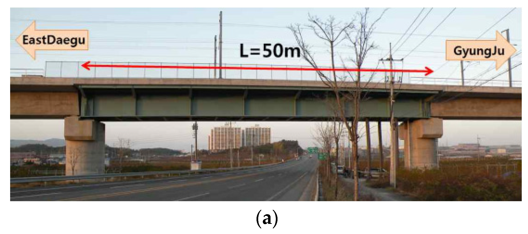
Kim
et al. [
5] designed a 3-D finite element model (FEM) of the Kaya Bridge using ANSYS V10.0 software (ANSYS, Canonsburg, PA, USA, 2005) to support the proposed movement analysis of different train’s speeds. Train speeds from 200 to 450 km/h were studied. The FEM model results are concluded as follows: (i) the natural frequency modes of the bridge are 3.186 (1st bending), 3.689 (2nd bending) and 5.913 (1st torsion) Hz for the first, second and third modes, respectively; (ii) the maximum vertical acceleration and displacement are 3.5 m/s
2 and 6 mm occurred with train speed 250 and 280 km/h, respectively; (iii) the maximum acceleration and displacement for the train 400 km/h speed are 1.6 m/s
2 and 3.8 mm, respectively. Therefore, comparing the FEM results and the bridge design criteria in
Table 1 shows that the bridge is safe under applied loads.
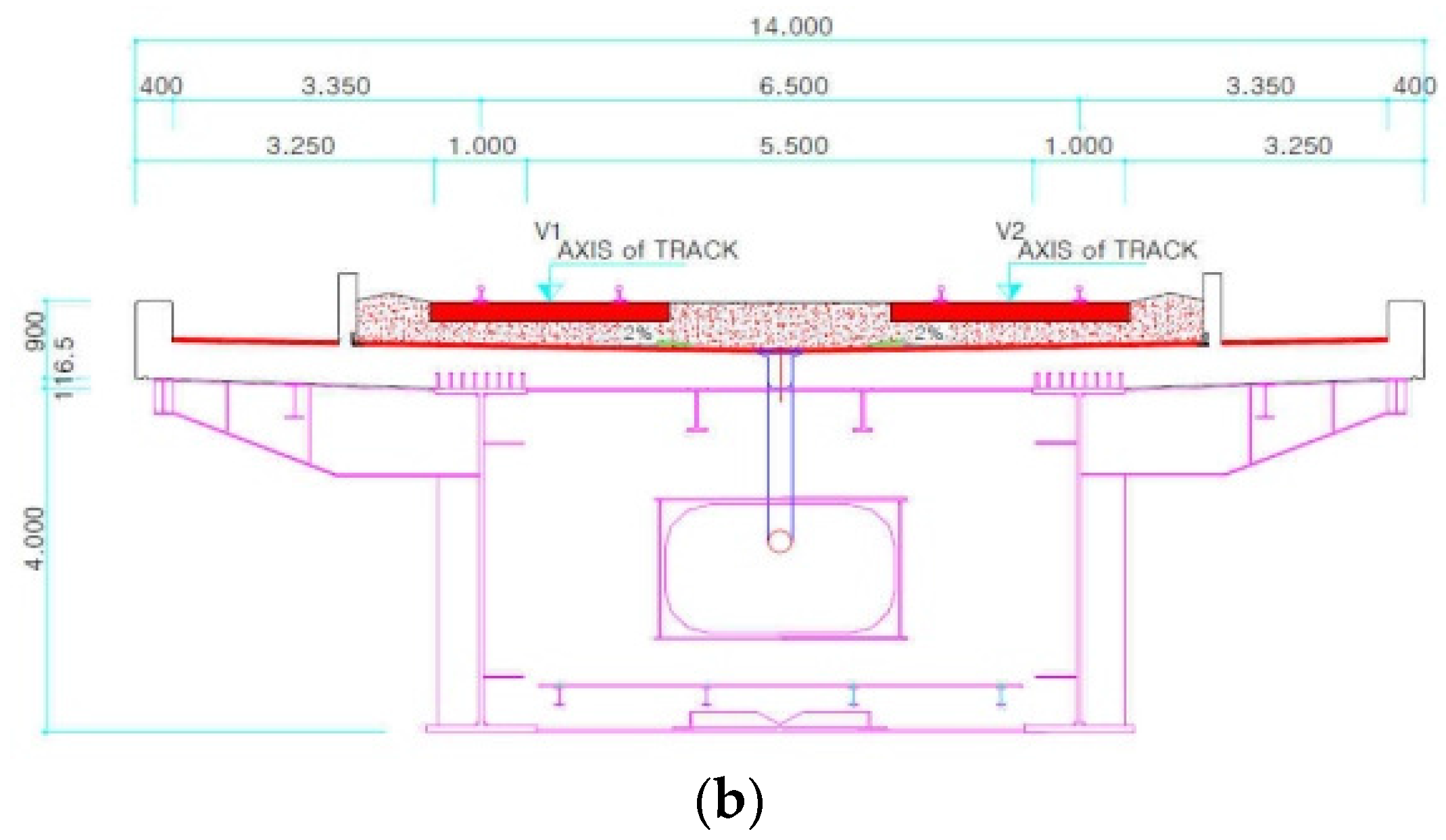
The current study utilizes the real monitoring data that is collected from the SHM system of Kaya Bridge to assess and evaluate the real bridge condition in terms of its vibration, static strain, torsional and fatigue behavior of the steel deck as well as evaluating and comparing the frequency contents for the measurements of the monitoring sensors.
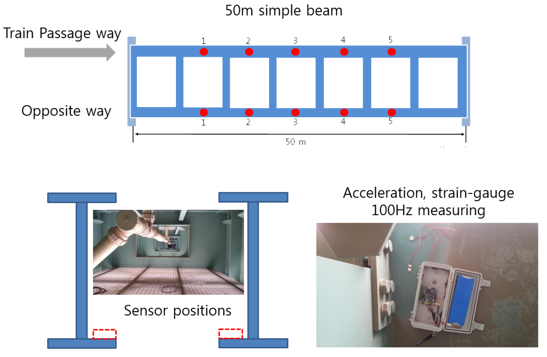
3.1. Evaluation of the Bridge Girder Vibration Behavior
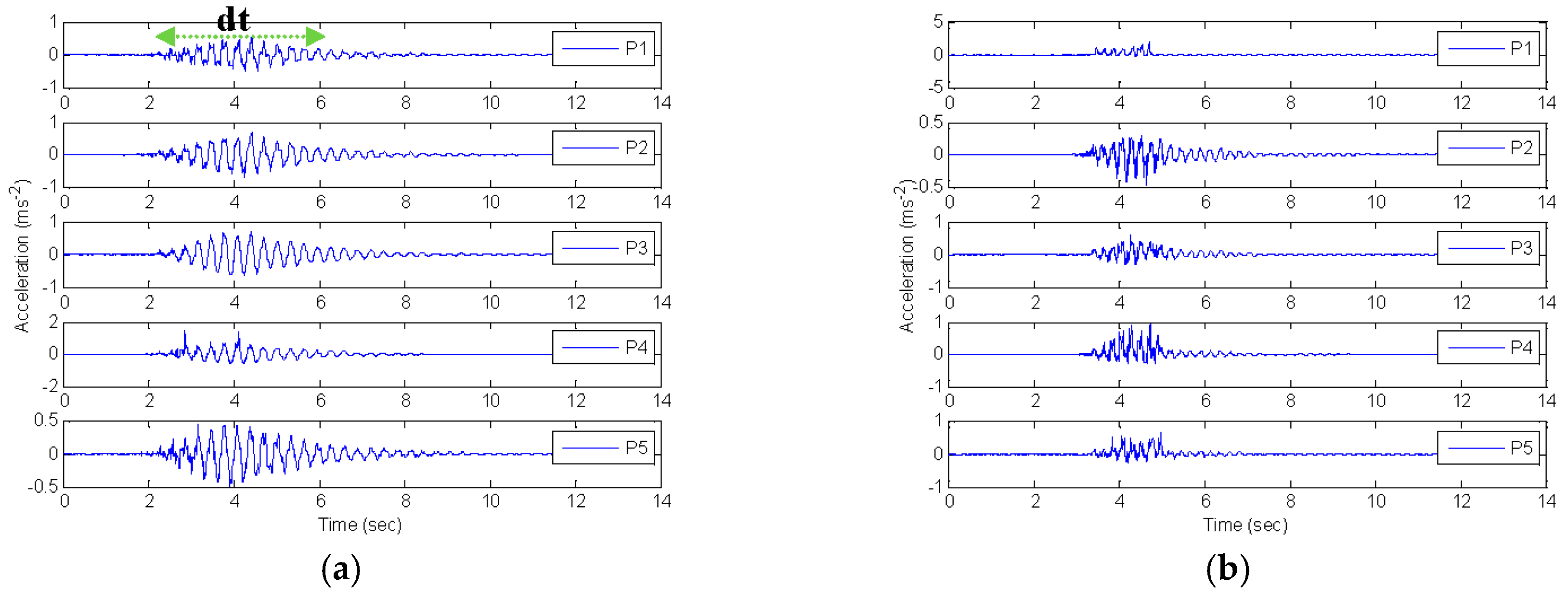
Figure 4a,b illustrate the typical vertical acceleration time histories of the passage monitoring points of the girder measured from accelerometers 1 to 5 for the 290 km/h and 406 km/h speed, respectively. It can be seen that the
dt, (
dt =
t2 (leave time) −
t1 (entrance time)) values are reported as 5.9, 2.92, 1.9 and 1.85 s with the speeds 290, 360, 400 and 406 km/h, respectively. This means that the vibration time effect on the bridge decreased by 68.65% as the train speed increased from 290 to 406 km/h. In addition, it is observed that the vibrations of the monitored points at a speed of 290 km/h are approximately the same, while as the speed increased, the entrance and exit monitoring points are experiencing high vibration response compared to the mid span point.
Figure 4.
Vertical acceleration time histories of the girder caused by a high-speed train. (a) passage response points for 290 km/h; (b) passage response points for 406 km/h.
Figure 4.
Vertical acceleration time histories of the girder caused by a high-speed train. (a) passage response points for 290 km/h; (b) passage response points for 406 km/h.
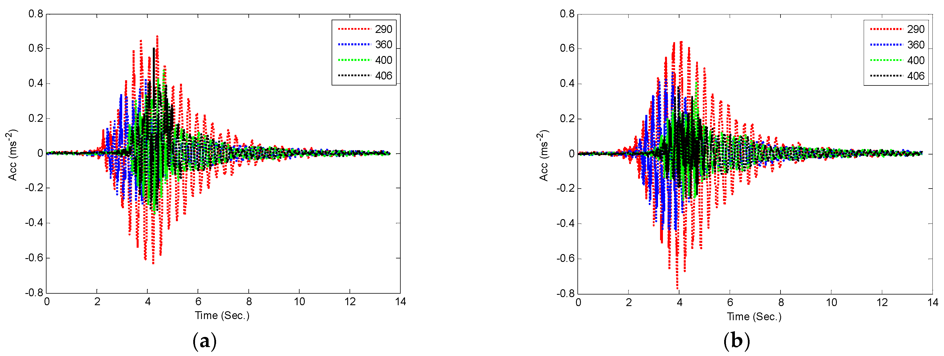
Figure 5 shows that the vertical acceleration of the mid-span point of the girder at 406 km/h is much smaller than that of 290 km/h. In addition, it is noticed that the vibration response for the passage way is higher than that of the opposite side at 400 and 406 km/h, while at 290 and 360 km/h, the acceleration responses for the passage and opposite sides are equal. These indicate that, although the structural layouts of the five monitoring points of the main girder are the same, there is a significant difference between the vertical vibration characteristics of two sides of the bridge due to the rail irregularity in the vertical directions with different speeds. Thus, there is a need to monitor the vertical accelerations of the span in the long term so as to realize anomaly alarms for vibration behavior of the main girder.In addition, the measured vertical acceleration is smaller than the FEM results by 62% according to the design criteria of the bridge (as shown
Table 1),which means that the real response is safe. Furthermore, the girder torsional behavior should be studied with new development trains’ speeds.
Figure 5.
Vertical acceleration time histories of the passage and opposite mid span girder point. (a) passage response of mid span point; (b) opposite response of mid span point.
Figure 5.
Vertical acceleration time histories of the passage and opposite mid span girder point. (a) passage response of mid span point; (b) opposite response of mid span point.
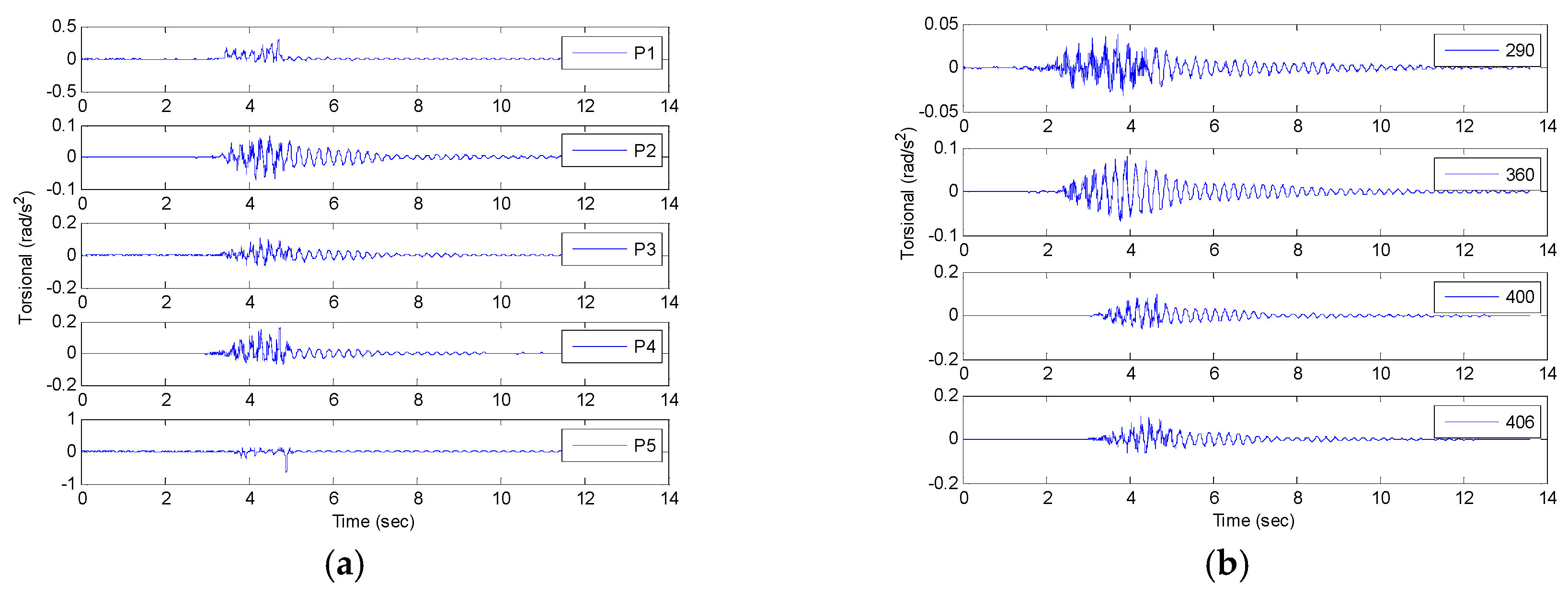
Figure 6 illustrates the dynamic torsional behavior of the bridge girder based on vertical acceleration measurements [
21].The torsional behavior of the girder due to train passage at 406 km/h is shown in
Figure 6a. While the torsional behavior of the mid span point at different speeds is shown in
Figure 6b.
where T,
and
l are the torsion, acceleration for the passage and opposite points and distances between sensors’ positions.
Figure 6.
Torsional measurements for the bridge girder. (a) the torsional of the monitoring points at 406 km/h passage; (b) mid span point torsional values.
Figure 6.
Torsional measurements for the bridge girder. (a) the torsional of the monitoring points at 406 km/h passage; (b) mid span point torsional values.
It is noticed that the torsional values increased as the train velocity increased with maximum values at points 1 and 5. As the speed increased from 290 to 406 km/h, the torsional values increased by 61.20%, while they increased by 22.33% as the train speed increased from 360 to 406 km/h. This means that the bridge deck torsional response is higher than the vibration response. The girder torsional value at the mid span point, 0.103 rad/s
2 , is within the design values, as shown in
Table 1.
The statistical parameters, maximum and root mean square (RMS), for the acceleration measurements and torsional calculations at 360 and 406 km/h are presented in
Table 2. The 360 km/h is assumed as the base-speed for the study of the bridge safety because the bridge design speed is 350 km/h. Furthermore, the Bessel filter cut-off frequency of 30 Hz is applied to remove the noise measurements of the accelerometer [
21]. It is noticed that the maximum acceleration occurred at points 1 and 5 for the passage and opposite directions at 406 km/h speed, respectively, with values within the design limits as shown in
Table 1. While there is no high relative change at points 2 to 4, the RMS of the 360 km/h is smaller than that of the 406 km/h on passage way, while
vice versa in the opposite way except for point 5. The maximum torsion occurred at point 5 at a speed of 406 km/h with a value very close to the design value (
Table 1). Thus, it is recommended to limit the train speed to 400 km/h only. In addition, the effective torsion test should be assessed at the end points of the bridge (point of maximum torsion).
Table 2.
Maximum acceleration, root mean square (RMS) and torsional acceleration for the filtration of vibration measurements.
Table 2.
Maximum acceleration, root mean square (RMS) and torsional acceleration for the filtration of vibration measurements.
| Point | Acceleration (m/s2) | RMS (m/s2) | Max Torsion (rad/s2) |
|---|
| Passage | Opposite | Passage | Opposite |
|---|
| 360 | 406 | 360 | 406 | 360 | 406 | 360 | 406 | 360 | 406 |
|---|
| 1 | 0.104 | 1.251 | 0.196 | 0.079 | 0.006 | 0.035 | 0.008 | 0.004 | 0.059 | 0.191 |
| 2 | 0.169 | 0.183 | 0.231 | 0.088 | 0.008 | 0.009 | 0.011 | 0.006 | 0.072 | 0.191 |
| 3 | 0.244 | 0.319 | 0.279 | 0.146 | 0.010 | 0.012 | 0.013 | 0.007 | 0.079 | 0.037 |
| 4 | 0.569 | 0.622 | 0.252 | 0.239 | 0.014 | 0.016 | 0.012 | 0.008 | 0.244 | 0.055 |
| 5 | - | 0.401 | 0.169 | 2.497 | - | 0.013 | 0.008 | 0.035 | - | 0.343 |
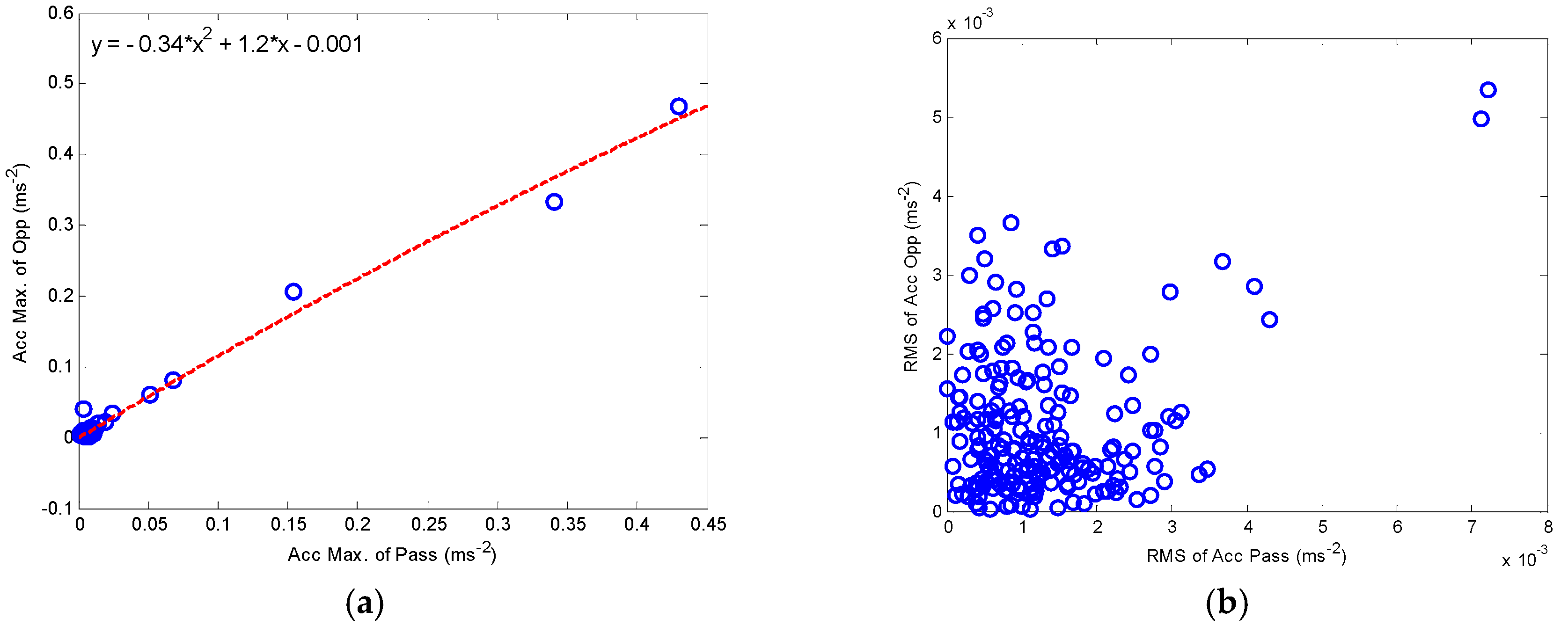
Ding
et al. [
3,
17] concluded that the quadratic linear fitting for the maximum and RMS are calculated for the acceleration measurements can be used to detect the performance of high-speed railway bridges based on one span monitoring. Herein, this method is applied to detect and check the performance of the bridge due to different speeds on the two ways of the track. The maximum and RMS of 150 acceleration of the original measurements are shown in
Figure 7. The quadratic linear fitting is suitable for the maximum acceleration (
Figure 7a), while the RMS shows no correlation between the passage and opposite ways. Therefore, the maximum acceleration fitting can be used to check the safety of the bridge.
Figure 7.
Cross-correlation between the passage and opposite way responses for 360 km/h. (a) cross-correlation maximum acceleration; (b) cross-correlation roote mean square (RMS) acceleration.
Figure 7.
Cross-correlation between the passage and opposite way responses for 360 km/h. (a) cross-correlation maximum acceleration; (b) cross-correlation roote mean square (RMS) acceleration.
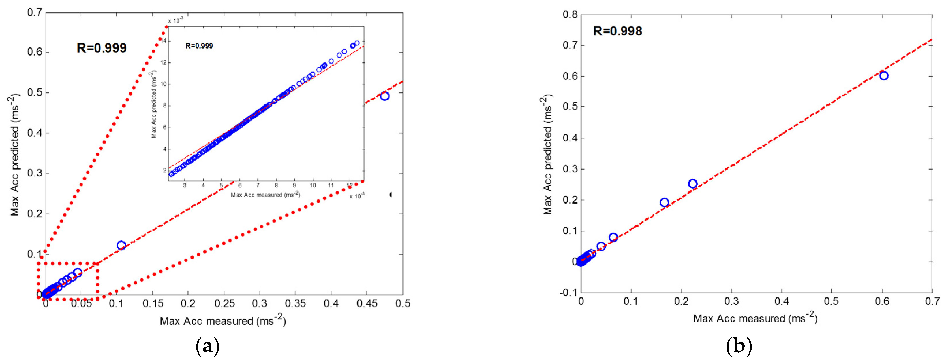
In this case, the fitting equation is used to predict the opposite way measurements for the 400 and 406 km/h, as shown in
Figure 8. The correlation coefficient of the measured maximum values and predicted values with 400 and 406 km/h is 0.999 and 0.998 for opposite accelerations, respectively. The results indicate that good cross-correlation exists between the maximum values of the opposite way at the two train speeds. Herein, the control chart can be used to monitor the changes in the vertical accelerations caused by deterioration of the vibration behavior. Firstly, the condition index
e (
e = Max (measurements) − Max (prediction)) for early warning of abnormal vibration behavior is defined as the difference between the measured and predicted maximum values of the accelerations in the opposite way. Then, a mean value control chart is employed to monitor the time series of
e with regard to the opposite accelerations. For online monitoring, the controlling parameter is chosen so that, when the structural vibration is in good condition, all observation samples fall between the control limits. When the new measurement is made, the structural abnormal vibration condition can be detected if an unusual number of samples fall beyond the control limits. In this study, the control condition is assumed with 290 km/h found within 0.025 to −0.03 m/s
2. The calculated condition index for the 400 and 406 km/h is between 0.0043 and −0.028 m/s
2. Hence, a long-term monitoring of the maximum values of the opposite accelerations can help in the early-warning of the vibration behavior deterioration. These results are identical with the Ding
et al. [
3,
17] conclusions.
Figure 8.
Predicting the effect of cross-correlation between maximum values of accelerations by using quadratic polynomials. (a) 400 km/h; (b) 406 km/h.
Figure 8.
Predicting the effect of cross-correlation between maximum values of accelerations by using quadratic polynomials. (a) 400 km/h; (b) 406 km/h.
3.2. Evaluation of the Bridge Girders’ Train Responses
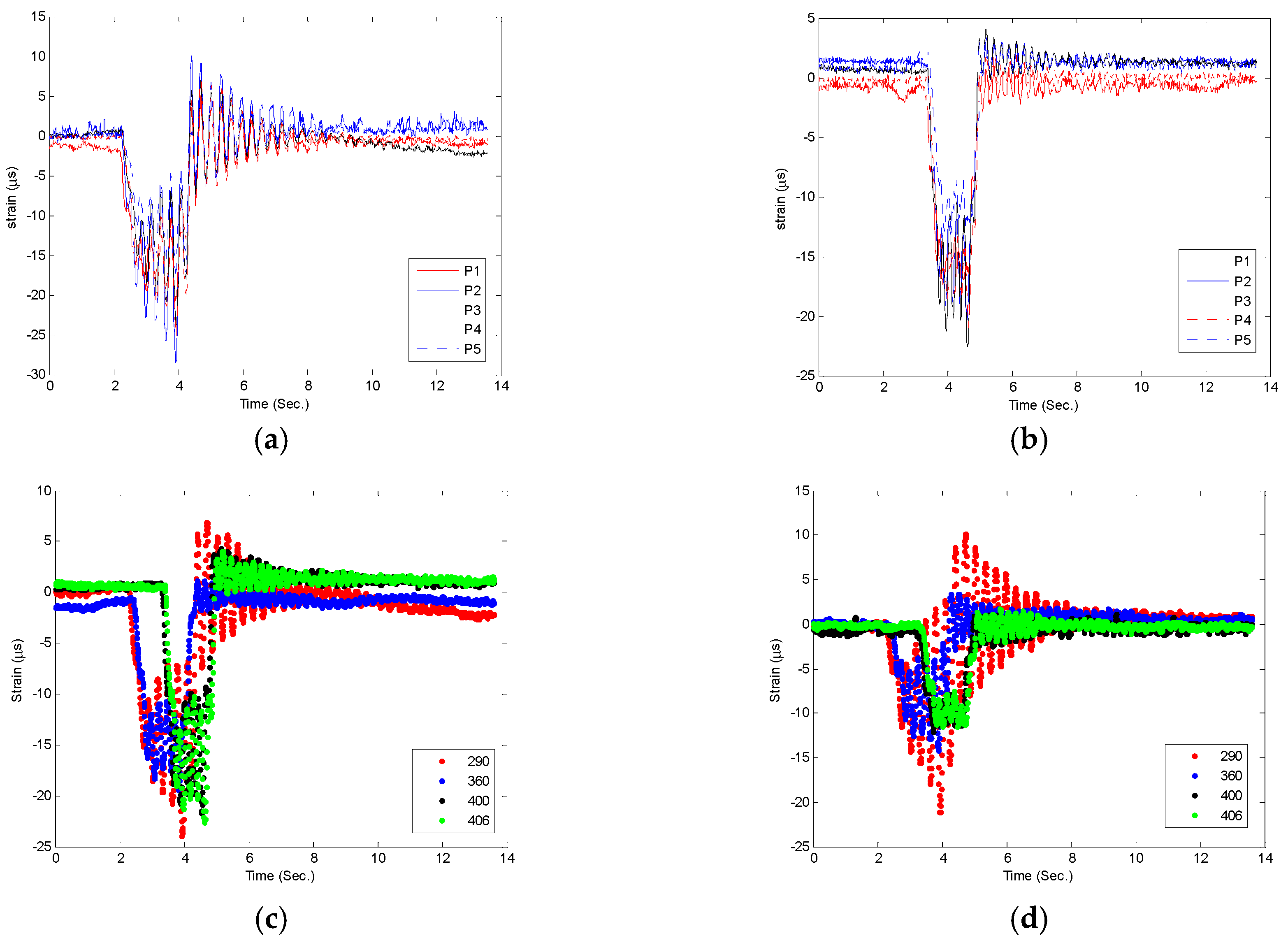
The measured vertical strain histories of the monitoring points of the passage way for the train speeds 290 and 406 km/h are presented in
Figure 9a,b. The vertical strain of the mid-span point of passage and opposite ways for different train speeds are compared in
Figure 9c,d. As the train speeds increase to 290, 360, 400 and 406 km/h, the strain responses (
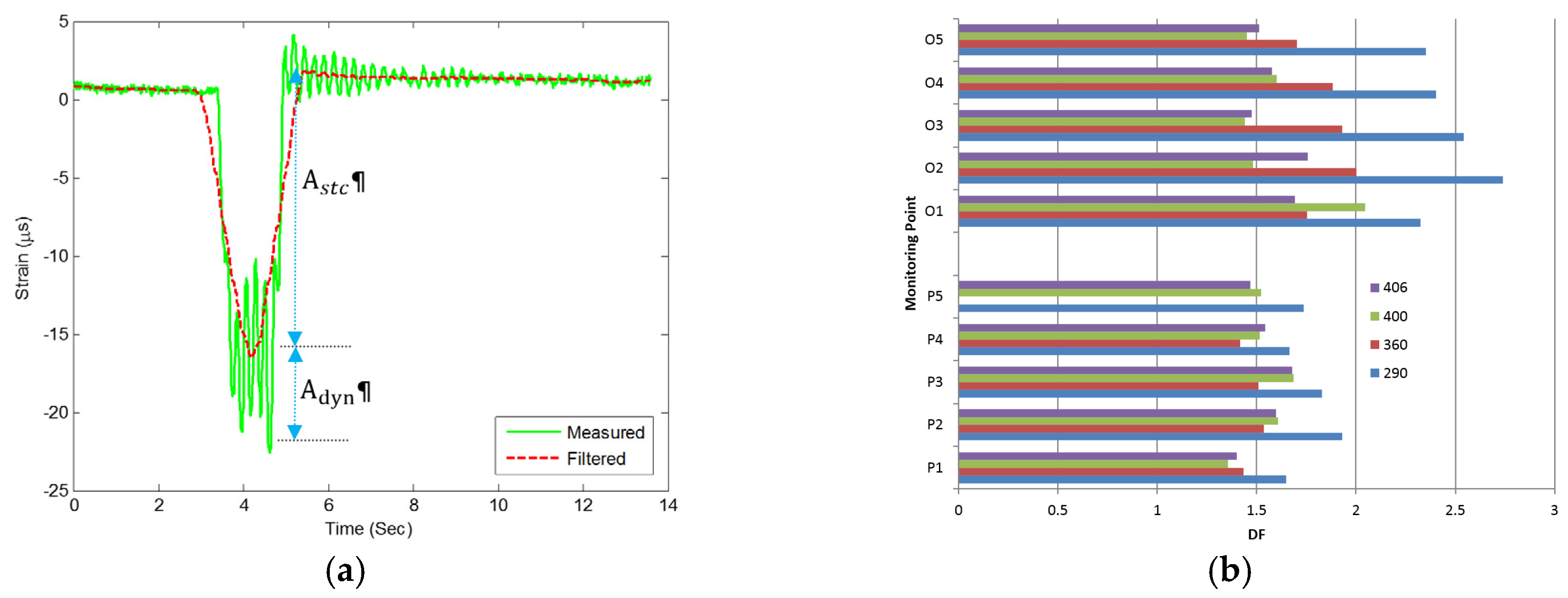
dt) decrease to 2.1, 1.93, 1.64 and 1.61 s, respectively. This shows that the time of static strain responses decreases by 23.33% when the speed changes from 290 and 406 km/h. In addition, the maximum strain response in the passage and opposite ways occurred at a speed of 290 km/h. The results as such show that the static and dynamic behavior of the bridge is higher with low train speeds. In addition, the strain measurements of the bridge points are highly correlated (0.95) with each speed change. This means that the strain measurement of the mid span point can be used to detect the performance of the whole bridge. This situation will decrease the cost of the monitoring system due to the use of one monitoring point only. The high correlation (0.99) of strain response for the passage and opposite ways occurred at 400 and 406 km/h. It means that the strain response of the two speeds is approximately equal in the static response. However, to show clearly the relationship between dynamic and static response of the bridge, the dynamic increment factor should be calculated and analyzed. The Savitzky-Golay finite impulse response(FIR) smoothing filter is applied to detect the static strain of the bridge. The first polynomial order with 101 frame size is utilized in this study.
Figure 10a shows the strain measurements and filter data of the mid span of passage direction with a train speed of 406 km/h. Therefore, the dynamic increment factor (DF) can be calculated as follows [
22,
23]:
where
and
are the maximum absolute of dynamic and static amplitude of the strain, as shown in
Figure 10a. The dynamic factors of passage (P) and opposite (O) directions for the monitored points are illustrated in
Figure 10b.
Figure 9.
Strain measurements of the main girder induced by high-speed train. (a) passing response points for 290 km/h; (b) passing response points for 406 km/h; (c) passage response mid span points; (d) opposite response mid span points.
Figure 9.
Strain measurements of the main girder induced by high-speed train. (a) passing response points for 290 km/h; (b) passing response points for 406 km/h; (c) passage response mid span points; (d) opposite response mid span points.
The dynamic factor calculation shows that the DF of 290 km/h train is higher than other train speeds at the passage and opposite directions. Furthermore, the DF of the opposite direction is higher than the passage direction with all train speeds except point (P3) with speeds of 400 and 406 km/h.
Figure 10.
Measured static strain and dynamic factor of the strain. (a) measured and filtered static strain; (b) dynamic factor of the monitoring points.
Figure 10.
Measured static strain and dynamic factor of the strain. (a) measured and filtered static strain; (b) dynamic factor of the monitoring points.
From
Figure 10b, it can be seen that the DFs for the development speeds are less than two. It means that the dominant performance of the bridge is static with speeds of 360, 400 and 406 km/h at all monitoring points, while the dynamic performance occurred at the opposite monitoring direction with train speed 290 km/h and point (O1) with train speed 400 km/h. These results indicate that the static behavior increases with increased train speeds. Therefore, the fatigue and frequency behavior should be studied to investigate the safety of the bridge under high train speed effect.
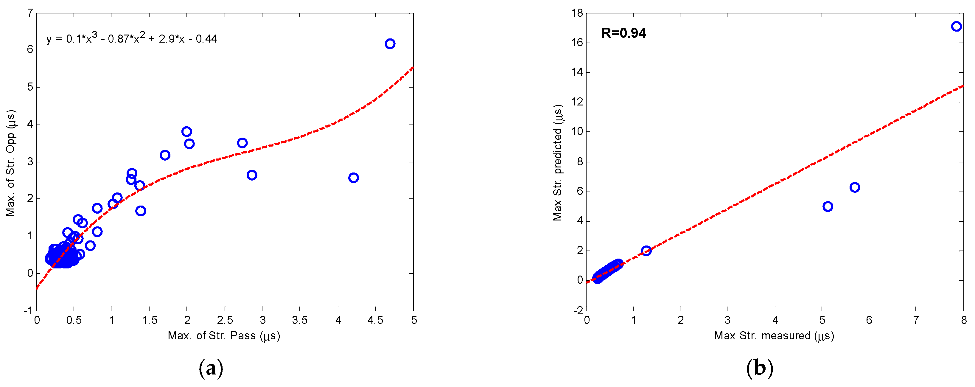
Herein, the cross-correlation evaluation is used to predict the dynamic behavior of strain contents. The same conditions used in the acceleration analysis are used in this part.
Figure 11 presents the cross-correlation and the cubic fitting of the maximum dynamic of strain measurements. The relationship between the maximum dynamic of strain contents in the passage and opposite directions for the train speed of 360 km/h is illustrated in
Figure 11a. While
Figure 11b shows the prediction of the opposite direction contents of the dynamic strain for 406 km/h, the statistical analysis of cubic and quadratic fitting shows that the correlation coefficient of quadratic is 0.90, so the cubic fitting in this case is better to predict the dynamic behavior of the strain contents. The comparison between the results of acceleration and strain dynamic contents shows that the dynamic evaluation of acceleration is better and effective to assess the vibration of the bridge, but the strain dynamic contents can be used to decrease the monitoring cost.
Figure 11.
Cross-correlation and prediction of maximum strain dynamic. (a) cross-correlation maximum dynamic of strain; (b) predicting effect of cross-correlation.
Figure 11.
Cross-correlation and prediction of maximum strain dynamic. (a) cross-correlation maximum dynamic of strain; (b) predicting effect of cross-correlation.
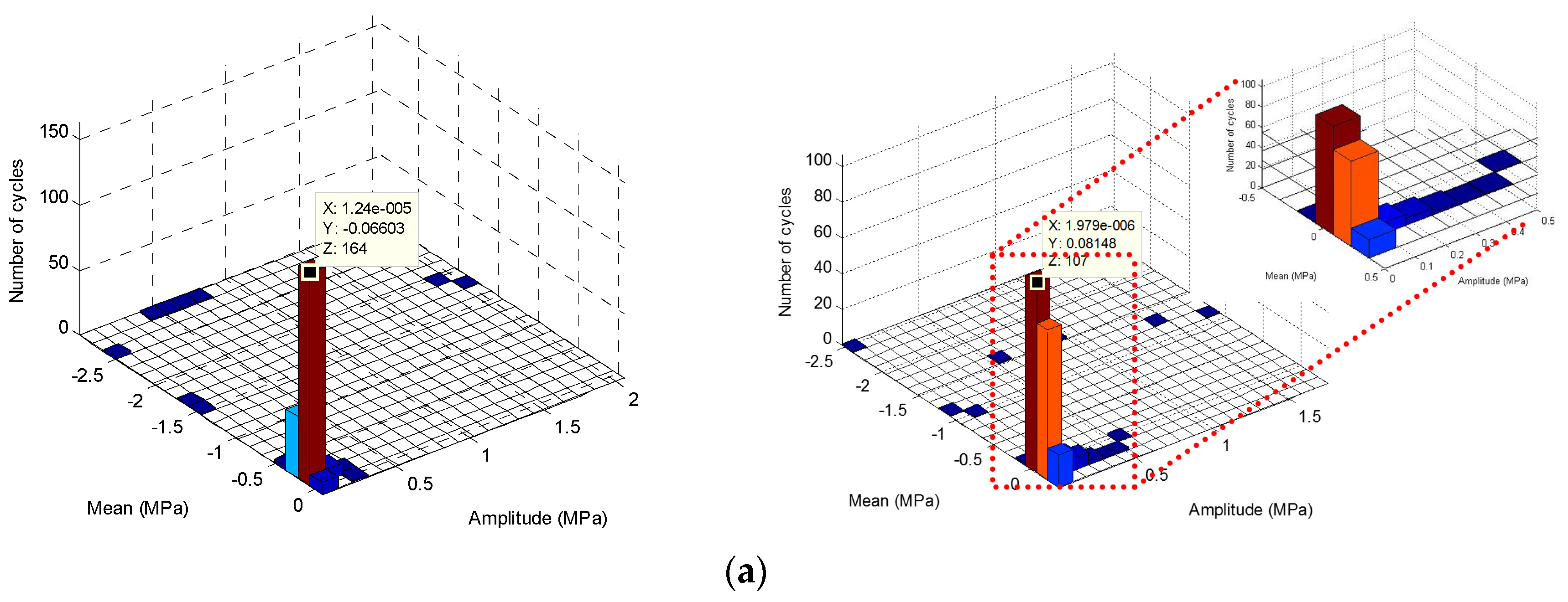
To perform fatigue evaluation, a simplified rain-flow cycle counting algorithm was used first to process strain history data and the spectrum of stress matrix obtained by statistical analysis [
17,
24]. The spectra of stress matrix calculated using the strain history data with train speeds of 360 and 406 km/h for the passage (left) and opposite (right) as shown in
Figure 12, respectively.In addition, the maximum stress cycles are presented in
Figure 12. It is observed that the maximum stress amplitude, obtained from strain history curves under two trains’ effects for the passage and opposite directions, is smaller than 2.5 MPa. Therefore, only a small number of stress cycles occur at the higher stress range. Most cycles occur in the region of stress mean and amplitude from −0.5 to 0.5 MPa and 0 to 0.5 MPa, respectively. Thus, the mean and amplitude values of the stress for the two trains in the two directions are equal.
Figure 12.
Rain-flow matrix of mid-span stress (a) 360 km/h; (b) 406 km/h.
Figure 12.
Rain-flow matrix of mid-span stress (a) 360 km/h; (b) 406 km/h.
The maximum number of stress cycles at 406 km/h is smaller than that occurring at 360 km/h in the two directions. The results show that the fatigue stress and number of cycles limit are 29 MPa and 2 × 10
6, respectively [
25], as recommended by Eurocode 3. The value of the equivalent stress amplitude and the number of cycles when the high-speed train passes through bridge is far less than this value for two trains. However, the fatigue behavior of the bridge deck satisfies the requirement of the infinite-fatigue-life design method.
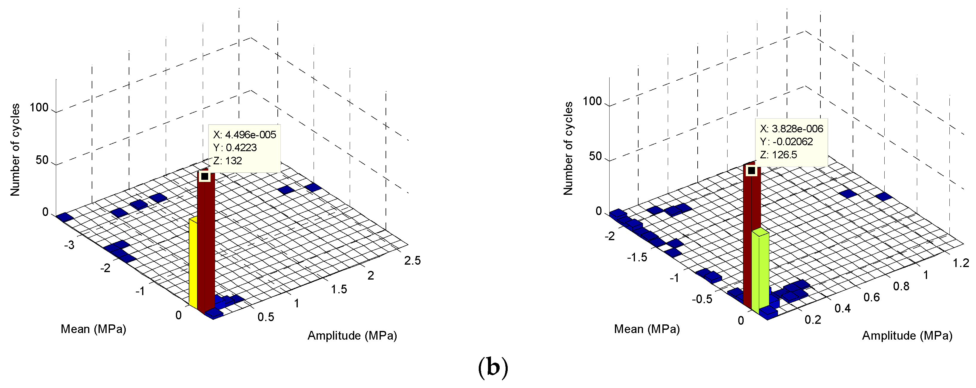
3.3. Acceleration-Strain Frequency Domain Evaluation
The frequency contents of strain and acceleration measurements for the mid-span monitoring points in the passage and opposite directions are illustrated in
Figure 13. The cross spectrum density function in Matlab (Version 7.6, MathWorks, Natics, MA, USA, 2008) is used to calculate the frequency contents.Based on the FEM [
5] analysis, the band-pass filters in between 1 to 45 Hz with 101 hamming window are used to filter the measured data to include the static and dynamic frequency contents of the bridge. From
Figure 13, the frequency contents are 3.223, 3.906 Hz and 3.223, 4.199 Hz for 290 and 360 km/h at the opposite and passage directions, respectively. In addition, the frequency contents equal (4.297 Hz) for the 400 and 406 km/h at the two directions. From the comparison of the FEM frequency and real data, it is observed that the first dynamic mode changes increased with increasing the trains’ speeds. The changes of passage frequency from the first bending FEM frequency mode are 18.5%, 24.2%, 25.8% for the speeds 290, 360 and 406 km/h, respectively. The strain frequencies contents at the two directions with the effect of all trains’ speeds are similar. In addition, the static frequency contents are clearly shown with strain measurements only. The low frequencies are 0.781, 0.977, 1.172, 1.172 Hz and 0.879, 1.074, 1.172, 1.172 Hz of the opposite and passage directions for the 290, 360, 400, 406 km/h train speeds, respectively. It means that the strain measurements are enough to estimate the static and dynamic behavior in frequency domain. Moreover, from the comparison between the first mode contents of the measurements and the FEM calculations, it can be concluded that the bridge is safe under its current dynamic behavior with the development speeds of trains.
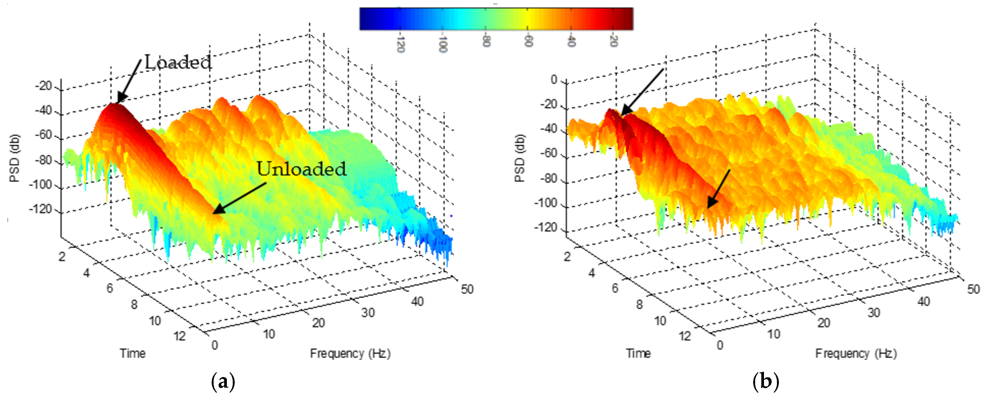
The Matlab Spectrogram toolbox is used to extract the three dimensional time-frequency maps for the passage train at the mid-span point of the bridge at speeds 290 and 406 km/h, as shown in
Figure 14. The results show that the power spectrum density (PSD) at 290 km/h speed is lower than the PSD amplitude at 406 km/h. The PSD frequency responses’ amplitude differences between trains passage and departure (load and unload) show small values at 406 km/h. Therefore, it is concluded that the dynamic behavior of the bridge at train speeds of 406 km/h is greater than the 290 km/h. However, it is concluded that the bridge is safe at a speed of 406 km/h, but it should be continuously monitored if trains speeds are increased above this value. Moreover, the increase of PSD with train speeds indicates that the simple beam girders of steel bridges are very sensitive to train induced vibrations, and, therefore, may be not suitable for an increase in the speed of train traffic.
Figure 13.
Acceleration and strain frequency contents. (a) passage-acceleration; (b) opposite-acceleration; (c) passage-strain; (d) opposite-strain.
Figure 13.
Acceleration and strain frequency contents. (a) passage-acceleration; (b) opposite-acceleration; (c) passage-strain; (d) opposite-strain.
Figure 14.
Time-frequency acceleration measurements for the trains speeds (a) 290 km/h and (b) 406 km/h.
Figure 14.
Time-frequency acceleration measurements for the trains speeds (a) 290 km/h and (b) 406 km/h.


