Agent Based Fuzzy T-S Multi-Model System and Its Applications

Abstract

Based on the basic concepts of agent and fuzzy T-S model, an agent based fuzzy T-S multi-model (ABFT-SMM) system is proposed in this paper. Different from the traditional method, the parameters and the membership value of the agent can be adjusted along with the process. In this system, each agent can be described as a dynamic equation, which can be seen as the local part of the multi-model, and it can execute the task alone or collaborate with other agents to accomplish a fixed goal. It is proved in this paper that the agent based fuzzy T-S multi-model system can approximate any linear or nonlinear system at arbitrary accuracy. The applications to the benchmark problem of chaotic time series prediction, water heater system and waste heat utilizing process illustrate the viability and the efficiency of the mentioned approach. At the same time, the method can be easily used to a number of engineering fields, including identification, nonlinear control, fault diagnostics and performance analysis.

1. Introduction

Along with the development of sensor technology, electro mechanical system and digital communication network, both the basis structure and run mode of engineering control system changed enormously [1,2]. These components of the engineering control systems are more intelligent, they will never act as the single role of controlled object or controller [3,4], instead an agent integrates sense, compute, execution and communication together. However, it also brings more uncertainty to the system, such as time variation and nonlinear characteristics. Therefore, the investigation of agent based fuzzy T-S multi-model system by the way of data information of the process is studied.

Many works have mentioned the idea of agent based modelling [5,6,7,8]. Different from the traditional model, the agent based modelling is formed by agents that lie in different layers [9]. There exists the interaction between the agents, and the input signals for an agent may be affected by the feedback information of others. Affecting other agents and affected by the others at the same time, the essence of the cooperation and interaction between different agents is the communication process of data information [10]. The communication channels between agents form the real time dynamic network. Within the network, each agent can execute the task alone or collaborate with other agents to obtain a fixed goal [11,12]. However, the control-oriented models of engineering systems call for further investigation.

Few attempts have been initiated in the study of the agent based fuzzy T-S multi-model system. In [13], a multi-agent consensus problem with an active leader and variable interconnection topology is studied. A neighbor-based local controller together with a neighbor-based state-estimation rule is given for each autonomous agent to track the leader. Then, a cooperative output regulation problem for linear uncertain multi-agent problem is studied in [14], and it shows a simple way of cooperation of the system if all subsystems of the agents have the same nominal dynamics. In [15], the fuzzy modelling and consensus problem of multi-agent nonlinear systems is analyzed. The T-S fuzzy models are proposed to express the system with variable structures. However, the agent based fuzzy multi-model strategy remains preliminary because how to construct the agents and lead all the agents in a multi-model system to reach a consensus is still a problem. More endeavors should be conducted in order to use the modelling strategy widely.

Starting from the basic concepts of agent and fuzzy T-S model, the agent based fuzzy T-S multi-model (ABFT-SMM) system is proposed in this paper. In this system, the agent that is described with a dynamic equation will be the local part of the multi-model, and the consensus of the agents accomplished by the center average defuzzifier. Moreover, we proved the ABFT-SMM could approximate any linear or nonlinear systems at arbitrary accuracy.

The structure of the rest of this paper is as following. In Section 2, several concepts of agents and fuzzy T-S model are introduced. In Section 3, the method for building agent based fuzzy multi-model is described in detail. In section 4, the approximation capability of the agent based fuzzy multi-model system is analyzed. Three different application examples are given in Section 5. Lastly, the conclusion is drawn in Section 6.

2. Concept Formulation

There are three main problems that need to be solved for establishing the ABFT-SMM system. Firstly, how a single agent can be built; Second, how the cooperation works among different agents; Third, how to combine the multi-model theory and the agent theory together. To solve these problems, here we will first introduce several basic but crucial concepts.

2.1. Dynamic Network of Agents

Defined $\mathcal{G}=(\nu ,\varsigma )$ is a weighted directed diagram, where ν is the set of node, ς is the frontier set. The nodes of the diagram are different agents whose state can be described with $x_i$, the process of the change of $x_i$ along with time can be expressed in a dynamic equation, and its time continuous form is

$${\dot{x}}_i(t)=f_i(x_i(t),u_i(t))$$

(1)

where $t\ge 0$, $i=1,...,N$. In addition, for discrete time form, the dynamic equation of each agent is

$$x_i(t+1)=f_i(x_i(t),u_i(t))$$

(2)

where $t=0,1,...$, $i=1,...,N$. Mark $\mathit{x}={(x_1,x_2,...,x_N)}^T$, then the two-tuple $\mathcal{G}=(\nu ,\varsigma )$ is combined together with $\mathit{x}$ to construct a dynamic network. The directed diagram $\mathcal{G}$ is called the communication topology or information flow diagram of the dynamic network.

2.2. Consensus Protocol

Definition 1: Let $\{x_i\in R,t\in \mathcal{T},i=1,...,N\}$ be N processes, where $\mathcal{T}$ is time index set, and in the time continue situation $\mathcal{T}=[0,\infty )$ , in discrete time situation $\mathcal{T}=\{t_0,t_1,...,t_j,...\}$, where $t_j(j=0,1,...)$ is monotone increasing of discrete time. If,

$$\underset{\mathcal{T}\ni t\to \infty }{lim}|x_i(t)-x_j(t)|=0$$

(3)

where $i,j=1,...,N$, then the dynamic network $(\mathcal{G},\mathit{x})$ is weak consensus.

Definition 2: Let $\{x_i\in R,t\in \mathcal{T},i=1,...,N\}$ be N processes, if there exists $x^{*}\in R$, lead

$$\underset{\mathcal{T}\ni t\to \infty }{lim}{x}_i(t)=x^{*}$$

(4)

where $i=1,...,N$, then the dynamic network $(\mathcal{G},\mathit{x})$ is strong consensus.

Definition 3: Let $h:R^N\to R$ be a function with N variables, and $\{x_i\in R,t\in \mathcal{T},i=1,...,N\}$ are N processes, if for arbitrary $x_i(0)(i=1,...,N)$, there will be

$$\underset{\mathcal{T}\ni t\to \infty }{lim}{x}_i(t)=h(x_1(0),x_2(0),...,x_N(0))$$

(5)

where $i=1,...,N$, then the dynamic network $(\mathcal{G},\mathit{x})$ is h-consensus. $h(x_1(0),x_2(0),...,x_N(0))$ is called the group decision value—especially, when $h(x_1(0),x_2(0),...,x_N(0))=\frac{1}{N}{\displaystyle \sum _{j=1}^N}{x}_j(0)$, is called as average consensus.

If the dynamic network $(\mathcal{G},\mathit{x})$ is weak consensus (strong consensus, h-consensus), and ν is called a weak consensus (strong consensus, h-consensus) protocol.

2.3. Fuzzy T-S Model

Fuzzy T-S model can be described as (6), it also be called the second kind of fuzzy T-S model [16],

$$\begin{array}{ccc}\hfill R^l:& & if{x}_{1}is{A}_1^{l}and{x}_{2}is{A}_2^{l}and...and{x}_{n}is{A}_n^l\hfill \end{array}$$

$$\begin{array}{ccc}& & then{y}^l=a_1^l{x}_1+a_2^l{x}_2+...+a_n^l{x}_n\hfill \end{array}$$

(6)

where $R^l$ is the $l^{th}$ fuzzy rule, $l=1,...,N$, N is the number of fuzzy rule, $A_i^l(i=1,...,n)$ is called the fuzzy subset, $\mathit{x}={(x_1,x_2,...,x_n)}^T$ and $y^l$ are the input and the output variables respectively, $a_i$ is the consequent parameter of local linear part. Compare with the first fuzzy T-S model, it brings many conveniences in computing process [17].

The output functions of the model can be described as following when the center average defuzzifier is adopted

$$y=\frac{{\displaystyle \sum _{l=1}^N}{\lambda }^l{y}^l}{{\displaystyle \sum _{l=1}^N}{\lambda }^l}$$

(7)

where $y^l$ is the output of the $l^{th}$ fuzzy set, ${\lambda }^l$ is the corresponding weight value.

Compared with the traditional modeling method, fuzzy rules based modeling method is a kind of multi-model way of modeling. Each rule of the fuzzy model can be seen as a local model, it means that the process of fuzzy modeling is the process of describing the action of the whole system by combining the local models [18,19].

3. Agent Based Fuzzy T-S Multi-Model System

It has been proved that the fuzzy T-S model can approximate any nonlinear systems at arbitrary accuracy in [17] and [20], At the same time, it has been proved that the second kind of fuzzy T-S model has the similar approximation capability with the first kind of fuzzy T-S model [21]. Here we use the linearized consequent of the fuzzy T-S model to express the dynamical equation of the agent. Combine formula (2) with (6), the agent based fuzzy model can be written as:

$$\begin{array}{ccc}\hfill R_i:& & if{x}_i(t)is{A}_{i1},x_i(t-1)is{A}_{i2},...\hfill \\ & & x_i(t-n+1)is{A}_{in},u_i(k-t_d)is{A}_{in+1},...,\hfill \\ & & u_i(k-t_d-m)is{A}_{in+m+1}\hfill \\ & & then{x}_i(t+1)=a_{i1}{x}_i(t)+a_{i2}{x}_i(t-1)+...+\hfill \\ & & a_{in}{x}_i(t-n+1)+a_{in+1}{u}_i(t-t_d)+...+\hfill \\ & & a_{in+m+1}{u}_i(t-t_d-m)\hfill \end{array}$$

(8)

where $R_i$ is the rule of agent i , and $A_k(k=i1,...,in+m+1)$ is the fuzzy subset, $a_{ik}$ is the consequent parameter of linear sub model.

The center average defuzzifier is adopted to the agent based fuzzy model, and then the agent based fuzzy T-S multi-model will be described as:

$$y=x(t+1)=\frac{{\displaystyle \sum _{i=1}^N}{\lambda }_i(\phi (k))x_i(t+1)}{{\displaystyle \sum _{i=1}^N}{\lambda }_i(\phi (k))}$$

(9)

where y is the system action which affected by the agents that instead the different work conditions, N is the number of the agents, $x_i(t+1)=f_i(x_i(t),u_i(t))$ is the dynamical equation of agent i and its linearized expression is like the output of (8), the expression of ${\lambda }_i(\phi (k))$ is corresponding to the membership value of agent i and it can be calculated from Gaussian bells function as (10).

$${\lambda }_i(\phi (k))=\exp [-\frac{{(\phi (k)-{\overline{c}}_i)}^T(\phi (k)-{\overline{c}}_i)}{s_i^2}]$$

(10)

where ${\phi }^T(k)=[-x_i(t),...,-x_i(t-n+1),u_i(k-t_d),...,u_i(k-t_d-m)]$ is $(n+m+1)$ dimensional row vector, n is the number of the agent states, m is the number of the past input states that relevant to current agent output, ${\overline{c}}_i\in R^{n_{\phi }}$ is the central variable of the Gaussian function, and $s_i$ is used to determine the width of the Gaussian function. Moreover, $s_i$ can be gotten in the following way

$$s_i=k_s\frac{1}{n}{\displaystyle \sum _{j=1}^n}|{\overline{c}}_i-{\overline{c}}_{ij}|$$

(11)

where ${\overline{c}}_{ij}$ is the $j^{th}$ neighbor center of the current center ${\overline{c}}_i$, and constant $k_s$ is used to determine the impact between deferent agents. Usually, the variation range of $s_i$ is not significant, and the value of $s_i$ can be chosen offline with the prior knowledge.

As analysed, in the modeling process, agents are h-consensus to the system output. A single agent is equivalent to a local network model. The cooperation among agents is accomplished by their membership value.

4. Universal Approximation Characteristics of Agent Based Fuzzy T-S Mutil-Model Systems

In this section, the approximation characteristic of ABFT-SMM system will be discussed. Without loss of generality, the continuous system of ABFT-SMM will be discussed first.

With (1), (9), the expression of the continuous system of ABFT-SMM can be expressed as follows:

$$\dot{x}(t)=\frac{{\displaystyle \sum _{i=1}^N}{\lambda }_i(x_i(t))f_i(x_i(t),u_i(t))}{{\displaystyle \sum _{i=1}^N}{\lambda }_i(x_i(t))}$$

(12)

where ${\lambda }_i(x_i(t))={\displaystyle \prod _{l=1}^{in+m+1}}\exp (-{(\frac{{\mathrm{z}}_{\mathrm{l}}-{\overline{\mathrm{z}}}_{\mathrm{l}}^{\mathrm{i}}}{{\mathrm{s}}_{\mathrm{i}}^{\mathrm{l}}})}^2)$, $z_l$ is the $l^{th}$ variable that effect agent i, here $l=1,...,(in+m+1)$ . Now we can get the following theorem:

Theorem 1: An ABFT-SMM system with product inference engine, singleton fuzzifier, center average defuzzifier, and Gaussian membership functions can uniformly approximate any linear or nonlinear continuous function on a compact set at arbitrary accuracy.

To prove this theorem, the famous Stone-Weierstrass theorem will be used.

Stone-Weierstrass Theorem [22]: Let Z be a set of real continuous functions on a compact set U. If, (i) Z is an algebra, that is, the set Z is closed under addition, multiplication, and scalar multiplication; (ii) Z separates points on U, that is, for every $x,y\in U,x\ne y$, there exists $f\in Z$ such that $f(x)\ne f(y)$; (iii) Z vanishes at no point of U, that is, for each $x\in U$ there exists $f\in Z$ such that $f(x)\ne 0$; then for any real continuous function $g(x)$ on U and arbitrary ϵ, there exists $f\in Z$ such that $\underset{x\in U}{\sup }|f(x)-g(x)|<ϵ$.

Proof of theorem 1: Let Y be the set of all fuzzy systems in the form of (12). We now show that Y is an algebra, Y separates points on the compact set U, and Y vanishes at no point of U. Firstly, we will prove Y is an algebra. Let $f_1,f_2\in Y$, and then $f_1,f_2\in Y$ can be written as:

$$f_1=\frac{{\displaystyle \sum _{i=1}^{N1}}{\lambda }_{1i}(\phi (k))f_{1i}(x_{1i}(t),u_{1i}(t))}{{\displaystyle \sum _{i=1}^{N1}}{\lambda }_{1i}(\phi (k))}$$

(13)

$$f_2=\frac{{\displaystyle \sum _{i=1}^{N2}}{\lambda }_{2i}(\phi (k))f_{2i}(x_{2i}(t),u_{2i}(t))}{{\displaystyle \sum _{i=1}^{N2}}{\lambda }_{2i}(\phi (k))}$$

(14)

Then, $f_1(x)+f_2(x)$ can be expressed as the form of (15),

$$f_1+f_2=\frac{{\displaystyle \sum _{l_1=1}^{N1}}{\displaystyle \sum _{l_2=1}^{N2}}2{\lambda }_{1i}{\lambda }_{2i}(f_{1i}+f_{2i})}{{\displaystyle \sum _{l_1=1}^{N1}}{\displaystyle \sum _{l_2=1}^{N2}}2{\lambda }_{1i}{\lambda }_{2i}}$$

(15)

where, $2{\lambda }_{1i}{\lambda }_{2i}$ can be seen as the input Gaussian membership function, $f_{1i}+f_{2i}$ is the dynamic equation of the agent. Obversely, (15) own the same structure with (12), it means that $f_1(x)+f_2(x)\in Y$. Similarly,

$$f_1{f}_2=\frac{{\displaystyle \sum _{l_1=1}^{N1}}{\displaystyle \sum _{l_2=1}^{N2}}{\lambda }_{1i}{\lambda }_{2i}(f_{1i}{f}_{2i})}{{\displaystyle \sum _{l_1=1}^{N1}}{\displaystyle \sum _{l_2=1}^{N2}}{\lambda }_{1i}{\lambda }_{2i}}$$

(16)

It is easy to know that $f_1{f}_2\in Y$. At the same time, when $c\in R$

$$c{f}_1=\frac{{\displaystyle \sum _{l=1}^{N1}}c{\lambda }_{1i}{f}_{1i}}{{\displaystyle \sum _{l=1}^{N1}}c{\lambda }_{1i}}$$

(17)

which is also in the same form with (12), so $c{f}_1(x)\in Y$. Then, we said that Y is an algebra.

Secondly, we prove that Y separates points on U. Construct a required fuzzy system $f(x)$, let $z^0,k^0\in U$ be two arbitrary points and $z^0\ne k^0$. The parameters of $f(x)=\dot{x}(t)$ in the form of (12) are chosen as $N=2,f_1=0,f_2=1,s_i^l=1,z_i^{*1}=z_i^0,z_i^{*2}=k_i^0(i=1,2,l=1,2,...,n)$. The established fuzzy system is as follows:

$$f(x)=\frac{\exp (-\parallel \mathrm{z}-{\mathrm{k}}^0{\parallel }_2^2)}{\exp (-\parallel \mathrm{z}-{\mathrm{z}}^0{\parallel }_2^2)+\exp (-\parallel \mathrm{z}-{\mathrm{k}}^0{\parallel }_2^2)}$$

(18)

and we can get (19) and (20) from (18)

$$f(z^0)=\frac{\exp (-\parallel {\mathrm{z}}^0-{\mathrm{k}}^0{\parallel }_2^2)}{1+\exp (-\parallel {\mathrm{z}}^0-{\mathrm{k}}^0{\parallel }_2^2)}$$

(19)

$$f(k^0)=\frac{1}{1+\exp (-\parallel {\mathrm{z}}^0-{\mathrm{k}}^0{\parallel }_2^2)}$$

(20)

Since $z^0\ne k^0$, then we can know $\exp (-\parallel {\mathrm{z}}^0-{\mathrm{k}}^0{\parallel }_2^2)\ne 1$, then it is easy to get that $f(z^0)\ne f(k^0)$. Therefore, Y separates points on U.

At last, we prove that Y vanishes at no point of U. It can be known from (12) that there always be $f(x)>0(\forall x\in U)$when $f_i(x_i(t),u_i(t)>0)$, hence

$$f(x)=\dot{x}(t)=\frac{{\displaystyle \sum _{i=1}^N}{\lambda }_i({\dot{x}}_i(t))f_i(x_i(t),u_i(t))}{{\displaystyle \sum _{i=1}^N}{\lambda }_i({\dot{x}}_i(t))}\ne 0$$

(21)

Combining the proof and Stone-Weierstrass theorem, the conclusion of theorem 1 can be obtained. While it is just the continuous time condition, the approximate ability will be discussed for the discrete system following:

Corollary 1: An ABFT-SMM system with product inference engine, singleton fuzzifier, center average defuzzifier, and Gaussian membership functions can uniformly approximate any linear or nonlinear discrete function on a compact set at arbitrary accuracy.

Proof of Corollary 1: Assume $h(x)$ is a square integrable function in compact set $U\in R^n$, and $g(x)\in L_2(U)=\{g(x):U\to R|{\int }_U{\left|g(x)\right|}^{2}dx<\infty$, combine with theorem 1, the following equation can be gotten

$$\left\{\begin{array}{c}{\int }_{U}dx<\infty \hfill \\ {({{\int }_U|g(x)-h(x)|}^{2}dx)}^{1/2}<\frac{ϵ}{2}\hfill \end{array}\right.$$

(22)

Then, it is easy to know that ${({\int }_U|g(x)-h(x)|}^2{dx)}^{1/2}<ϵ$.

More details about the approximate characteristic of the fuzzy model can be found in [20], while it mentioned the traditional fuzzy system. Here, we draw the collusion form theorem 1 and corollary 1 that ABFT-SMM can approximate any linear or nonlinear system at arbitrary accuracy, and it means that the ABFT-SMM system is a universal approximator. Thus, the proposed method could be widely used in a number of fields, such as behavior modeling, adaptive nonlinear control, fault detection and diagnostics. This paper could be a theoretical foundation for the implementation of ABFT-SMM systems in practical applications.

5. Applications and Discussions

To demonstrate the accuracy of ABFT-SMM to approximate the nonlinear system, the method is applied to a benchmark problem named chaotic Mackey-Glass time series prediction, a case of identification of the electrical water heater system and the modeling of waste heat utilizing process, respectively.

5.1. Chaotic Time Series Prediction

5.1.1. Description of the Equation

The benchmark problem of model identification, predicting the time series generated by the chaotic Mackey-Glass differential delay equation, can be expressed as follows [23,24,25,26,27,28,29]:

$$\dot{x}(t)=\frac{ax(t-\tau )}{1+x^{10}(t-\tau )}-bx(t)$$

(23)

The task of this example is to predict the output of some fixed steps later with past states of x, the value of the signal 24 steps ahead $x(t+24)$ is predicted based on the current signal value. Consider the Mackey-Glass problem as a process plant, parameters a, b and τ will vary in different working condition points. Assume there are three working conditions for the process, the parameter values of the plant are outlined in Table 1, where $x(0)$ is the initial value of the nonlinear system.

Table 1. Parameters of Mackey-Glass example under three different working conditions.

Conditions	a	b	τ	$x(0)$
1	0.2	0.1	17	1.2
2	0.2	0.09	19	1.0
3	0.2	0.12	16	0.7

Table 1. Parameters of Mackey-Glass example under three different working conditions.

Conditions	a	b	τ	$x(0)$
1	0.2	0.1	17	1.2
2	0.2	0.09	19	1.0
3	0.2	0.12	16	0.7

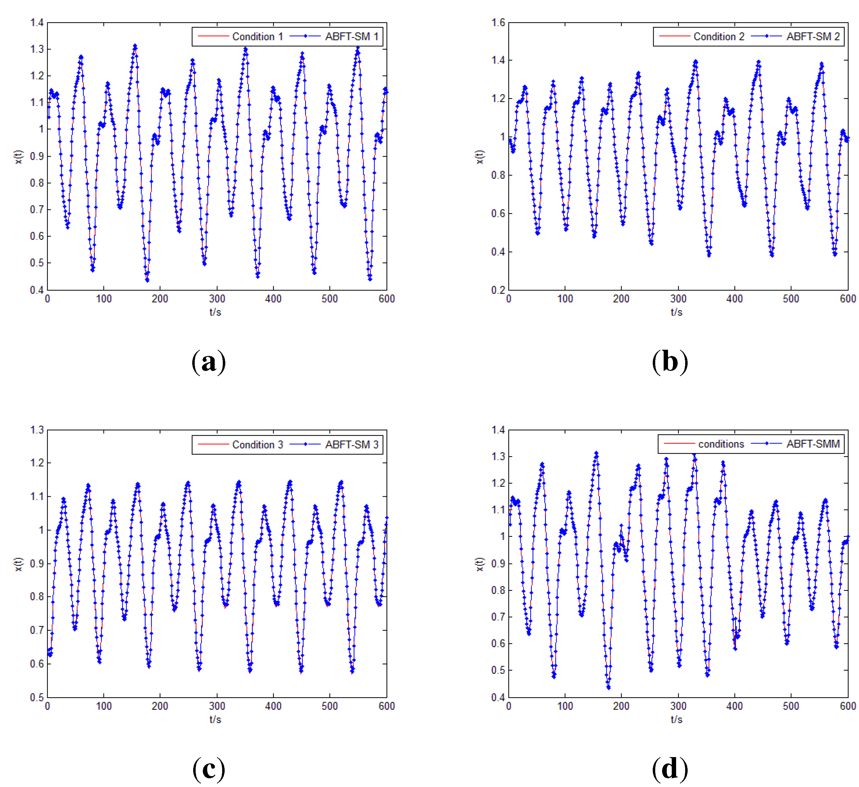
5.1.2. Simulation Tests

As analyzed in Section 3, agents corresponding to the models of different working conditions. Therefore, the models of Mackey-Glass problem under different working conditions can be approached with the agent based fuzzy T-S models (sort by ABFT-SM). In this example, 600 data samples from $t=101$ to $t=700$ are used to illustrate the method. The output signal values of the six steps ahead are shown in Figure 1.

Figure 1a–c are corresponding to the working condition 1 to 3 respectively. The outputs of ABFT-SM 1 to ABFT-SM 3 matched the fixed condition curves smoothly, which means that the agents can run effectively in fixed working conditions. The main initial values and indexes of the prediction systems of different conditions are listed in Table 2, where $r_a$ is the cluster radius of the agents, both $r_a$ and $s_i$ are the initial values of the method, centers are the structure index and root mean square error (RMSE) is the performance index of the system.

Figure 1d shows the tracking result of the ABFT-SMM, where the 600 data samples are consisted with three different conditions. The first 200 data samples come from condition 1, the second 200 data samples from condition 2, and the third 200 data samples from condition 3. The centers for the agents are calculated in different conditions, so here the number of the centers for the fuzzy T-S multi-model is 19. The RMSE of the ABFT-SMM in this time is 0.0056, it is very close to the accuracy of the single condition, and the computation complexity is proper.

Figure 1. Comparison of the ABFT-SM identification results with Mackey-Glass time series outputs. (a) is the tracking result for condition 1, (b) is the tracking result for condition 2, (c) is the tracking result for condition 3, and (d) is the varied condition situation.

Figure 1. Comparison of the ABFT-SM identification results with Mackey-Glass time series outputs. (a) is the tracking result for condition 1, (b) is the tracking result for condition 2, (c) is the tracking result for condition 3, and (d) is the varied condition situation.

Table 2. Initial values and the indexes of the prediction systems.

Conditions	$r_a$	$s_i$	Centers	RMSE
1	0.14	0.1	7	0.0037
2	0.1	0.1	6	0.0044
3	0.19	0.1	6	0.0040

Table 2. Initial values and the indexes of the prediction systems.

Conditions	$r_a$	$s_i$	Centers	RMSE
1	0.14	0.1	7	0.0037
2	0.1	0.1	6	0.0044
3	0.19	0.1	6	0.0040

5.1.3. Comparison and Discussion

Above all, both the tracking curve and the RMSE index indicate that the ABFT-SMM method runs efficiently in the working condition changed situation. It proves that the predictive outputs followed the process very well. At the same time, the modeling error, with respect to the data of condition 1, is listed in Table 3 along with the results from other methods as reported in [23,26,27,28,29]. Comparison between various methods shows that the ABFT-SMM can reach a better degree of accuracy. That is because different agents can collaborate to describe the nonlinear process, moreover, the membership values of the agents can be adjusted online when new data comes to the system.

Table 3. Comparison of results from different existed methods.

Methods	Data	RMSE
ABFT-SMM	600	0.0037
Cluster Estimation-Based [23]	500	0.014
ANFIS [26]	500	0.007
eTS [28]	300	0.0925
IT2FNN [29]	500	0.0053
Linear Predictive Method [27]	2000	0.55

Table 3. Comparison of results from different existed methods.

Methods	Data	RMSE
ABFT-SMM	600	0.0037
Cluster Estimation-Based [23]	500	0.014
ANFIS [26]	500	0.007
eTS [28]	300	0.0925
IT2FNN [29]	500	0.0053
Linear Predictive Method [27]	2000	0.55

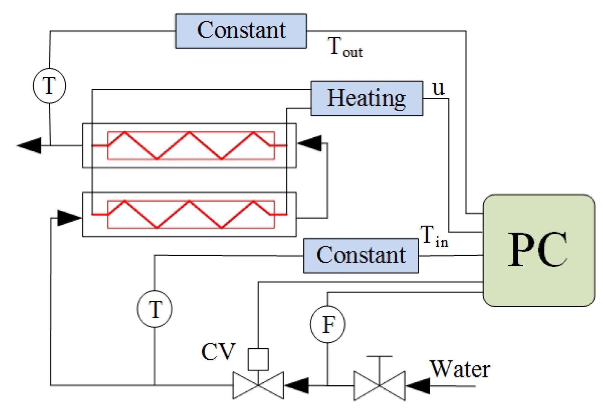
5.2. Identification of Electrical Water Heater

5.2.1. Description of the System

The schematic diagram of the water heater system is shown in Figure 2. The flow rate of cold water, F, which comes from the pipeline is controlled by the valve CV. Next, the cold water flows through a pair of metal pipes containing a cartridge heater. The outlet temperature, $T_{out}$, of the water can be varied by adjusting the heating signal, u , of the cartridge heater [30]. To physical modeling, there are four parts in the circle: the cartridge-heater (subscript h), the streaming water (subscript w), the pipe wall (subscript p) and the environment (subscript e). The following three heat balances in the form of partial differential equations can be established:

$$\left\{\begin{array}{c}{V}_h{\rho }_h{C}_{ph}\frac{\partial T_h}{\partial t}(t,z)=Q(u)-{\alpha }_1{A}_1(T_h-T_w)\hfill \\ V_w{\rho }_w{C}_{pw}\frac{\partial T_w}{\partial t}(t,z)+{(F_{\rho }{C}_p)}_w\frac{\partial T_w}{\partial z}(t,z)={\alpha }_1{A}_1(T_h-T_w)-{\alpha }_2{A}_2(T_w-T_p)\hfill \\ V_p{\rho }_p{C}_{pp}\frac{\partial T_p}{\partial t}(t,z)={\alpha }_2{A}_2(T_w-T_p)-{\alpha }_e{A}_e(T_p-T_e)\hfill \end{array}\right.$$

(24)

where, V is volume, ρ is density, C is specific heat, Q is the heat power, α is heat transfer coefficient, A is area, T is temperature, and F is flow rate. Here, $z\in [1,L]$ with L being the length of the pipe. Additional, Q is nonlinear with the manipulated heating signal, while it can be approximated with a generalized linear dynamics function described as:

$$G(z)=\frac{b_1{z}^{-1}+b_2{z}^{-2}}{1-a_1{z}^{-1}-a_2{z}^{-2}}+{\nu }_0$$

(25)

where a and b are the coefficients of the model, ${\nu }_0$ is the initial value. Two different conditions mentioned in [30] are listed in Table 4, and the parameters will change with the process.

Figure 2. Schematic diagram of water heater system.

Figure 2. Schematic diagram of water heater system.

Table 4. Parameters of water heater example under different working conditions.

Conditions	$a_1$	$a_2$	$b_1$	$b_2$	${\nu }_0$
1	$-1.8$	0.8112	0.0093	0.0019	20.83
2	$-1.817$	0.8302	0.0032	0.0086	21.35

Table 4. Parameters of water heater example under different working conditions.

Conditions	$a_1$	$a_2$	$b_1$	$b_2$	${\nu }_0$
1	$-1.8$	0.8112	0.0093	0.0019	20.83
2	$-1.817$	0.8302	0.0032	0.0086	21.35

5.2.2. Simulation and Discussion

In this example, 700 data samples from $t=101$ to $t=800$ are used to test the method. The results of the identification are shown in Figure 3. It shows that the agents can run effectively in a fixed working condition. The main initial values and indexes of the identification systems under different conditions are list in Table 5. The 700 data samples of Figure 3c are consisted with two different conditions, The first 350 data samples come from condition 1, the second 350 data samples from condition 2. The RMSE of the ABFT-SMM in this time is 0.0107. It is very close to the RMSE value of condition 1 or condition 2, which means the ABFT-SMM method runs efficiently in the condition-changed situation, while more complex systems need to be used to test the approach.

Table 5. Initial values and indexes of the identification systems.

Conditions	$r_a$	$s_i$	Centers	RMSE
1	0.18	1	21	0.01
2	0.2	1	17	0.0096

Table 5. Initial values and indexes of the identification systems.

Conditions	$r_a$	$s_i$	Centers	RMSE
1	0.18	1	21	0.01
2	0.2	1	17	0.0096

Figure 3. Comparison of the ABFT-SM identification results with heater system outputs. (a,b) are corresponding to the working condition 1 and 2 respectively; (c) is the varied condition situation.

Figure 3. Comparison of the ABFT-SM identification results with heater system outputs. (a,b) are corresponding to the working condition 1 and 2 respectively; (c) is the varied condition situation.

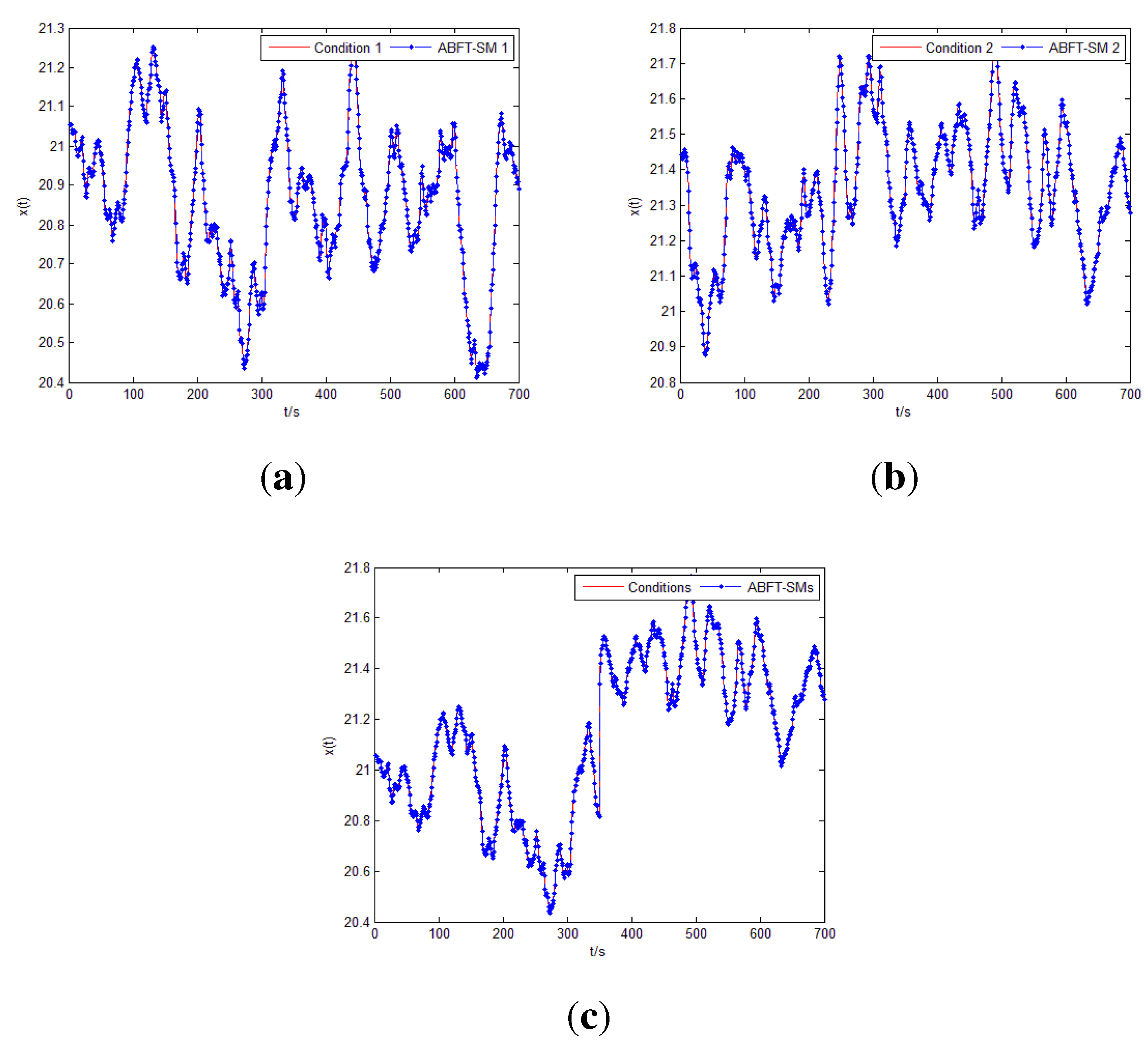
5.3. Waste Heat Utilizing System Modeling

5.3.1. System Description

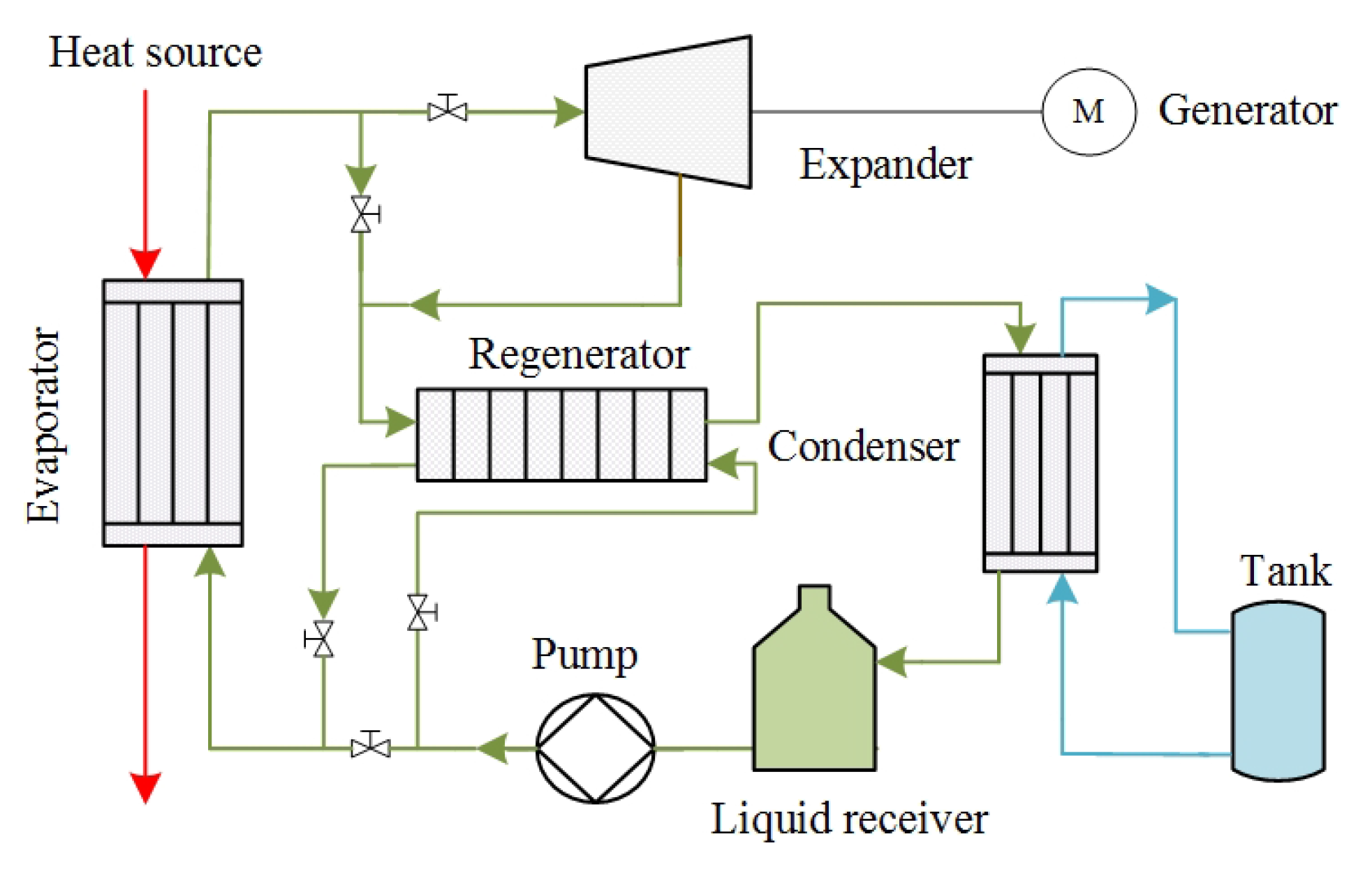
An application of modeling the 11 kW waste heat utilizing system is studied in this section, and the conceptual diagram of the power generate process is shown in Figure 4. In the system, R123 whose critical properties listed in Table 6 is selected as the working fluid. The energy of the waste heat source is transferred to the working fluid in the evaporator, and then the vaporized R123 enters the turbine and drives it to generate power. The working fluid vapor from the expander is next used to preheat the cold working fluid in a regenerator before it enters the evaporator. The vapor from the regenerator is then condensed back into liquid state in a water-cooled condenser. The liquid stored in a receiver then is pumped into the regenerator again.

The physical model of the waste heat utilizing system can be drawn from the partial differential equations of the mass balance and the energy balance, while there are many strong nonlinear components in the circle, such as evaporator, condenser and some electrical valves. The system evolved by physical modeling and traditional identification modeling strategy usually cannot match the needs of the control system when the work condition varies; therefore, the agent based fuzzy identification method for waste heat utilizing system is investigated in this paper. In general, the nonlinear expression of this process is as follows:

$$y_k=f(y_{k-1},...,y_{(}k-n_A),u_k,u_{k-1},...,u_{k-n_B},{\xi }_k)$$

(26)

where, $y_k$ is the output of the system, $u_k$ is the input, and ${\xi }_k$ is the random disturb.

Figure 4. Conceptual diagram of the waste heat utilizing system.

Figure 4. Conceptual diagram of the waste heat utilizing system.

Table 6. Critical properties of R123.

Molecular Formula	CHCl2CF3
Molecular weight	152.931 g/mol
Critical pressure	3.662 MPa
Critical temperature	456.681 K
Critical density	550.004 kg/m3

Table 6. Critical properties of R123.

Molecular Formula	CHCl2CF3
Molecular weight	152.931 g/mol
Critical pressure	3.662 MPa
Critical temperature	456.681 K
Critical density	550.004 kg/m3

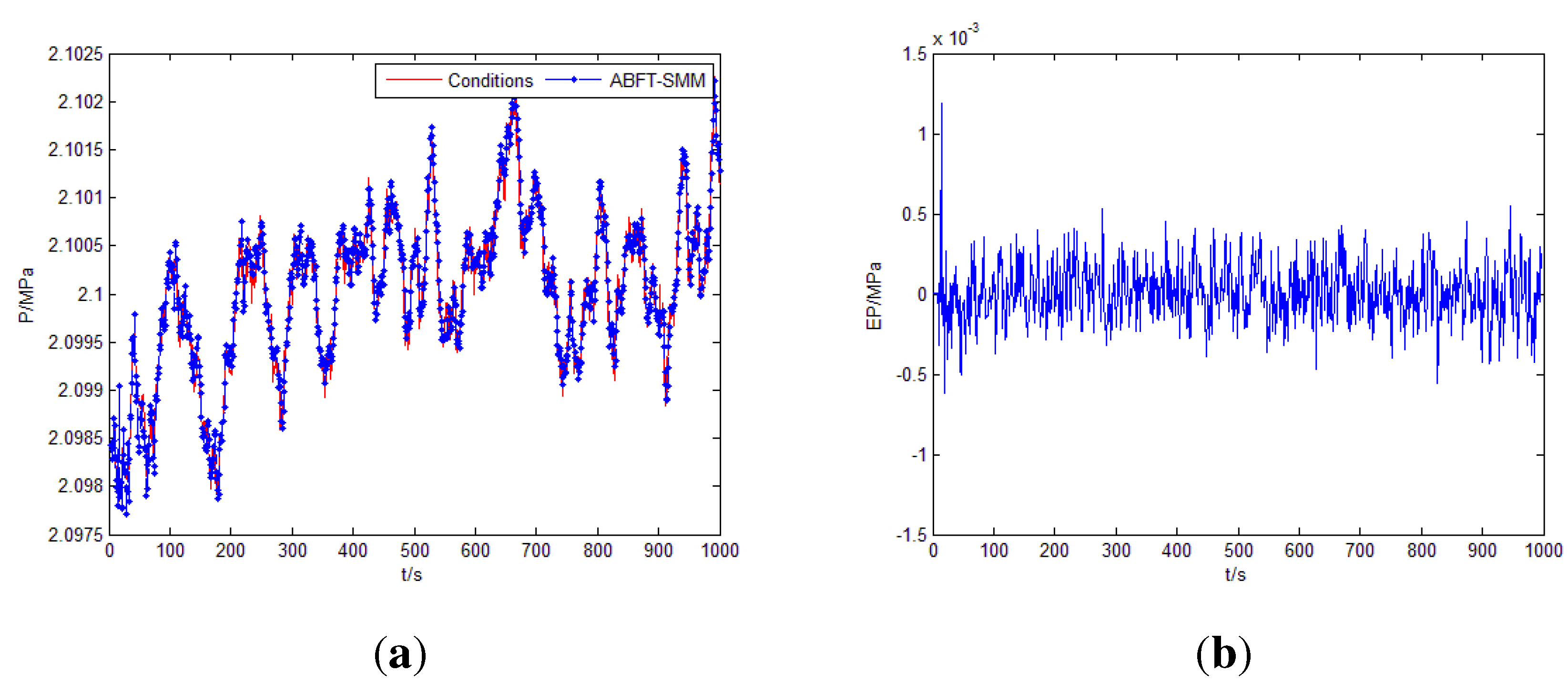
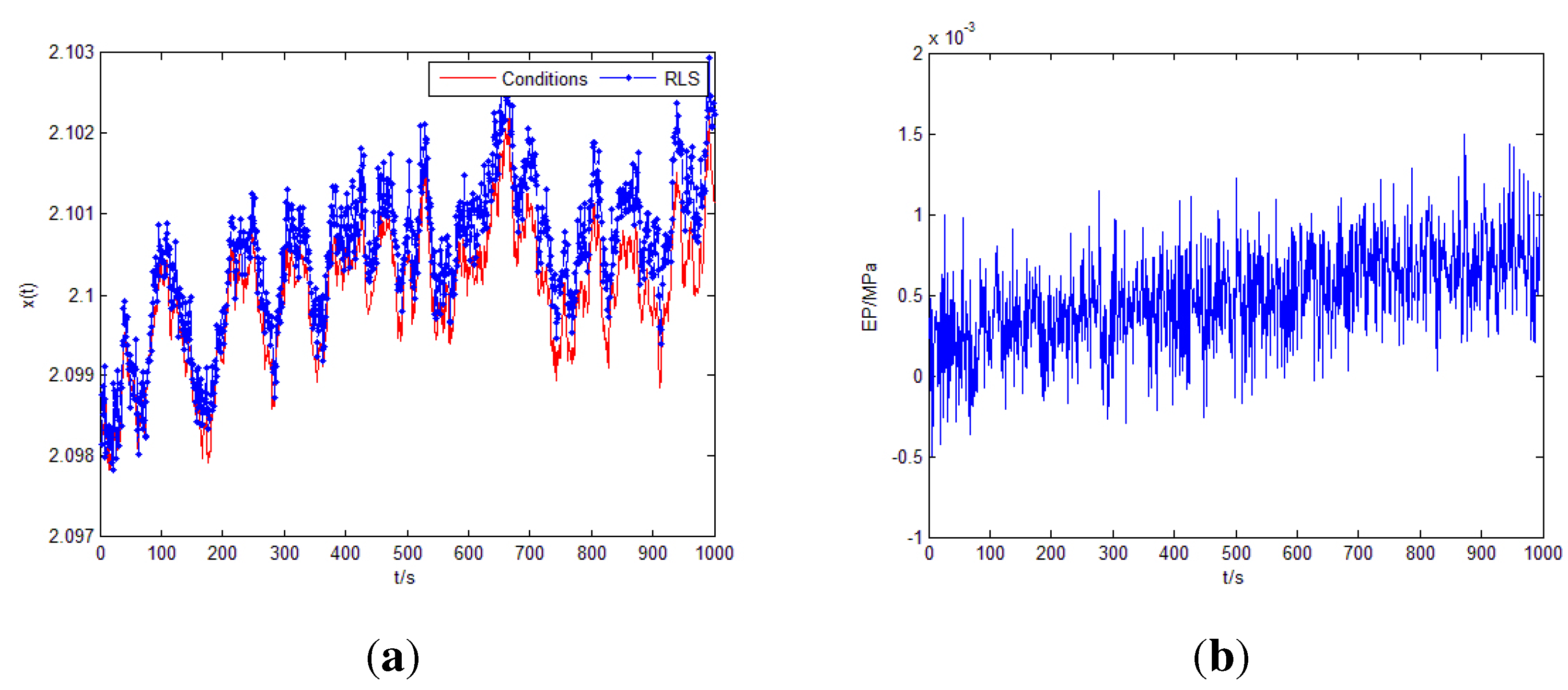
5.3.2. Simulation Tests

Consider the whole system, the evaporating pressure and the superheating temperature are the main variables that should be regulated to improve the efficiency of the system and keep safety of the components. After running, we find that the evaporating pressure is mainly adjusted by the expander speed and the superheating by the fluid pump speed, and the channel of evaporating pressure is studied here. The zero mean write noise is adopted as the identification signal, and 1000 data samples are chosen in 1 s sampling interval when the pump speed runs from 500 rad/min to 550 rad/min. The comparison curve of the ABFT-SMM outputs with the actual system outputs are shown in Figure 5.

Figure 5. Comparison of the ABFT-SMM outputs with the actual system outputs. (a) is the tracking curve of the identification model; (b) is the tracking error.

Figure 5. Comparison of the ABFT-SMM outputs with the actual system outputs. (a) is the tracking curve of the identification model; (b) is the tracking error.

5.3.3. Comparison and Discussion of System Performances

The parameters of the identified model and its performance index are shown in Table 7. It can be known from the modeling curve and the performance index that the agent based online multi-model method can model the nonlinear waste heat utilizing process efficiently. In order to test the performance of the mentioned approach, an recursive least square (RLS) method simulation result is shown in Figure 6. It is clear that all the performances of the ABFT-SMM system are better (have the smaller criteria values) than those of the RLS system. These superiorities benefited from the multi-model based structure and the parameter adjust characteristics of the agents. The application result shows an accurate and stable performance, it provides a good foundation for detection and control of the system.

Figure 6. Comparison of the RLS outputs with the actual system outputs.

Figure 6. Comparison of the RLS outputs with the actual system outputs.

Table 7. Parameters and the indexes of the identification model.

$a_1$	$a_2$	$a_3$	$a_4$	$a_5$	$a_6$	Centers	RMSE
$-0.4641$	$-0.2905$	$-0.2148$	$5.299\times {10}^{-5}$	$3.954\times {10}^{-5}$	$2.440\times {10}^{-5}$	8	$1.783\times {10}^{-4}$

Table 7. Parameters and the indexes of the identification model.

$a_1$	$a_2$	$a_3$	$a_4$	$a_5$	$a_6$	Centers	RMSE
$-0.4641$	$-0.2905$	$-0.2148$	$5.299\times {10}^{-5}$	$3.954\times {10}^{-5}$	$2.440\times {10}^{-5}$	8	$1.783\times {10}^{-4}$

6. Conclusions

In this paper, an ABFT-SMM system is established, and the approximation characteristic of the system is discussed. The concepts of agent and fuzzy T-S model are first addressed to describe the structure of the ABFT-SMM system. Different from the traditional method, the parameters and the membership value of the agent can be adjusted along with the process, which lead to application results better than the existing studies. Then, both the approximation capability of continuous and discrete systems are analyzed with the famous Stone-Weierstrass theorem. Finally, chaotic time series prediction, water heater identification and waste heat utilizing process modeling are presented to illustrate the viability and efficiency of the mentioned approach.

The following conclusions can be drawn:

(1)

The ABFT-SMM system is an h-consensus network.

(2)

The structure of the model can be adjusted by the number of the agents and their corresponding weights.

(3)

The proposed modelling method can approximate any linear or nonlinear system at arbitrary accuracy.

References

1. McArthur, S.D.; Davidson, E.M.; Catterson, V.M. Multi-Agent Systems for Power Engineering Applications—Part I: Concepts, Approaches,and Technical Challenges. IEEE Trans. Power Syst. 2007, 22, 1743–1752. [Google Scholar] [CrossRef] [Green Version]
2. Parker, J.; Epstein, J.M. A Distributed Platform for Global-Scale Agent-Based Models of Disease Transmission. ACM Trans. Model Comput. Simul. 2011, 22, 1–33. [Google Scholar] [CrossRef] [PubMed]
3. Romanovski, I.; Caines, P.E. On the supervisory control of multi-agent product systems: Controllability properties. Syst. Control Lett. 2007, 56, 113–121. [Google Scholar] [CrossRef]
4. Muller, S.C.; Hager, U.; Rehtanz, C. A Multiagent System for Adaptive Power Flow Control in Electrical Transmission Systems. IEEE Trans. Ind. Informat. 2014, 10, 2290–2299. [Google Scholar] [CrossRef]
5. Oh, H.S.; Thomas, R.J. Demand-Side Bidding Agents: Modeling and Simulation. IEEE Trans. Power Syst. 2008, 39, 1050–1056. [Google Scholar]
6. Bristow, M.; Fang, L.P.; Hipel, K.W. Agent-Based Modeling of Competitive and Cooperative Behavior Under Conflict. IEEE Trans. Syst. Man Cybern. Syst. 2014, 44, 834–850. [Google Scholar] [CrossRef]
7. Cheng, Z.M.; Zhang, H.T.; Fan, M.C.; Chen, G.R. Distributed Consensus of Multi-Agent Systems With Input Constraints: A Model Predictive Control Approach. IEEE Trans. Circuits Syst. I 2015, 62, 1549–8328. [Google Scholar] [CrossRef]
8. Doctor, F.; Iqbal, R.; Naguib, R.N.G. A fuzzy ambient intelligent agents approach for monitoring disease progression of dementia patients. J. Ambient Intell. Humaniz. Comput. 2014, 5, 147–158. [Google Scholar] [CrossRef] [Green Version]
9. Dai, P.P.; Liu, C.L.; Liu, F. Consensus Problem of Heterogeneous Multi-agent Systems with Time Delay under Fixed and Switching Topologies. Int. J. Autom. Comput. 2014, 11, 340–346. [Google Scholar] [CrossRef]
10. Hu, J.P.; Liu, Z.X.; Wang, J.H.; Lin, W.; Hu, X.M. Estimation, intervention and interaction of multi-agent systems. Acta Autom. Sin. 2013, 39, 1796–1804. [Google Scholar] [CrossRef]
11. Hong, Y.G.; Chen, G.R.; Bushnell, L. Distributed observers design for leader-following control of multi-agent networks. Automatica 2008, 44, 846–850. [Google Scholar] [CrossRef]
12. Wang, B.C.; Zhang, J.F. Distributed control of multi-agent systems with random parameters and a major agent. Automatica 2012, 48, 2093–2106. [Google Scholar] [CrossRef]
13. Hong, Y.G.; Hu, J.P.; Gao, L.X. Tracking control for multi-agent consensus with an active leader and variable topology. Automatica 2006, 42, 1177–1182. [Google Scholar] [CrossRef]
14. Su, Y.F.; Hong, Y.G.; Huang, J. A General Result on the Robust Cooperative Output Regulation for Linear Uncertain Multi-Agent Systems. IEEE Trans. Autom. Control 2013, 58, 1275–1279. [Google Scholar] [CrossRef]
15. Xiong, W.J.; Yu, W.W.; Lv, J.H.; Yu, X.H. Fuzzy Modelling and Consensus of Nonlinear Multiagent Systems With Variable Structure. IEEE Trans. Circuits Syst. I 2014, 61, 1183–1191. [Google Scholar] [CrossRef]
16. Ying, H. General SISO Takagi-Sugeno Fuzzy Systems with Linear Rule Consequent Are Universal Approximators. IEEE Trans. Fuzzy Syst. 1998, 6, 582–587. [Google Scholar] [CrossRef]
17. Angelov, P.; Filev, D. An approach to online identification of Takagi-Sugeno fuzzy models. IEEE Trans. Syst. Man Cybern. 2004, 34, 484–498. [Google Scholar] [CrossRef]
18. Narendra, K.S.; Xiang, C. Adaptive Control of Discrete-Time Systems Using Multiple Models. IEEE Trans. Autom. Control 2000, 45, 1669–1686. [Google Scholar] [CrossRef]
19. Rosyadi, M.; Muyeen, S.M.; Takahashi, R.; Tamura, J. A Design Fuzzy Logic Controller for a Permanent Magnet Wind Generator to Enhance the Dynamic Stability of Wind Farms. Appl. Sci. 2012, 2, 780–800. [Google Scholar] [CrossRef]
20. Wang, L.X. Fuzzy Systems are Universal Approximators. In Proceding of the IEEE International Conference on Fuzzy Sysystem, San Diego, CA, USA, 8–12 March 1992; pp. 1163–1170.
21. Zhang, H.G.; Liu, D.R. Fuzzy Modeling and Fuzzy Control; Birkhauser: Basel, Switzerland, 2006. [Google Scholar]
22. Rudin, W. Principles of Mathematical Analysis; Publishing House: McGraw-Hill, Inc.: New York, NY, USA, 1976. [Google Scholar]
23. Chiu, S.L. Fuzzy model identification based on cluster estimation. J. Int. Fuzzy Syst. 1994, 2, 267–278. [Google Scholar]
24. Abonyi, J.; Babuska, R.; Szeifert, F. Modified Gath-Geva Fuzzy Clustering for Identification of Takagi-Sugeno Fuzzy Models. IEEE Trans. Syst. Man Cybern. B Cybern. 2002, 32, 612–621. [Google Scholar] [CrossRef] [PubMed]
25. Kalhor, A.; Araabia, B.N.; Lucasa, C. Evolving Takagi-Sugeno fuzzy model based on switching to neighboring models. Appl. Soft Comput. 2013, 13, 939–946. [Google Scholar] [CrossRef]
26. Jang, J. ANFIS: Adaptive-network-based fuzzy inference system. IEEE Trans. Syst. Man Cybern. 1993, 23, 665–685. [Google Scholar] [CrossRef]
27. Crowder, R. Predicting the Mackey-Glass Time Series with Cascade-Correlation Learning. In Proceding of the 1990 Summer School, Carnegie Mellon University, Pittsburgh, PA, USA, January 1990; pp. 117–123.
28. Angelov, P.; Xydeas, C.; Filev, D. Online identification of MIMO Evolving Takagi-Sugeno fuzzy models. IEEE Trans. Syst. Man Cybern. 2004, 1, 55–60. [Google Scholar]
29. Castillo, O.; Castro, J.R.; Melin, P.; Diaz, A.R. Application of interval type-2 fuzzy neural networks in non-linear identification and time series prediction. Soft Comput. 2014, 18, 1213–1224. [Google Scholar] [CrossRef]
30. Abonyi, J. Fuzzy Model Identification for Control; Birkhauser: Basel, Switzerland, 2003; pp. 243–245. [Google Scholar]