Article

Research on the Fault Coefficient in Complex Electrical Engineering

1
Hebei Electric Power Research Institute, Shijiazhuang, Hebei 050022, China
2
State Key Laboratory of Alternate Electrical Power System with Renewable Energy Sources, North China Electric Power University, Beijing 102206, China
3
Interdisciplinary Mathematics Institute, University of South Carolina, Columbia, SC 29208, USA
*
Author to whom correspondence should be addressed.
These authors contributed equally to this work.
Appl. Sci. 2015, 5(3), 307-319; https://doi.org/10.3390/app5030307
Submission received: 13 April 2015 / Accepted: 3 August 2015 / Published: 7 August 2015

Abstract

:
Fault detection and isolation in a complex system are research hotspots and frontier problems in the reliability engineering field. Fault identification can be regarded as a procedure of excavating key characteristics from massive failure data, then classifying and identifying fault samples. In this paper, based on the fundamental of feature extraction about the fault coefficient, we will discuss the fault coefficient feature in complex electrical engineering in detail. For general fault types in a complex power system, even if there is a strong white Gaussian stochastic interference, the fault coefficient feature is still accurate and reliable. The results about comparative analysis of noise influence will also demonstrate the strong anti-interference ability and great redundancy of the fault coefficient feature in complex electrical engineering.

1. Introduction

Fault detection is always one of the core problems in the complex electrical engineering field. Generally speaking, fault detection can be divided into three categories based on analytical models, signal processing, and knowledge [1,2,3,4,5]. Among these fault detection technologies, the analytical models based fault detection technology was the earliest development and the most systematical research. It can construct a system model based mainly on the connections between components in a composition system and can be roughly divided into state estimation method, parameter estimation method and equivalence space method [6,7,8]. The fault detection based on signal processing can avoid establishing an object’s mathematical model, and it can directly analyze measurable information by signal model, such as correlation function, frequency spectrum, high order statistics, autoregressive moving average process and so on. The fault can be detected by extracting amplitude, variance, frequency and other characteristic values [9,10]. The fault detection based on signal processing mainly includes principle component analysis method, absolute value testing, tendency testing, Kullback detection, self-adaptable filter detection, etc. Similar to signal processing based fault detection, the fault detection based on knowledge is mainly applied to a nonlinear system. At the knowledge level, on the basis of knowledge processing technologies, the dialectical logic and mathematical logic will be integrated, and the symbol processing and numerical processing will be unified. It will also mainly include an expert system, fuzzy reasoning, neural network and rough set, etc. [11,12,13,14].
In fact, whichever fault detection technology we will adopt, the effective extraction of the fault feature is always the key problem. According to complex electrical engineering, we have carried out large numbers of basic research [15,16,17,18]. In this paper, based on the fundamental of feature extraction about the fault coefficient, we will discuss the fault coefficient in complex electrical engineering.
The paper is organized as follows. In Section 2, the fundamental of feature extraction about fault coefficient are introduced. In Section 3, the Phasor Measurement Unit and Wide Area Measurement System are described, and they have provided a real-time data platform for improving the security and stabilization of power system. In Section 4, for general fault types in complex electrical engineering, the feature extraction process of fault coefficient is clarified in detail. Finally, the paper is concluded in Section 5.

2. The Fundamental of Feature Extraction about the Fault Coefficient

For general, fault factor model [19,20],
x i = μ i + a i 1 f 1 + a i 2 f 2 + + a i m f m + ε i                  ( i = 1 , 2 , , n )
where f 1 , f 2 , , f m are m fault factors (common factor), a i j is the loading of x i on f j , μ i is mean value of x i , and ε i is specific factor of x i .
If x is a random vector that each component has been standardized, then the correlation coefficient between x i and f j is
ρ ( x i , f j ) = C o v ( x i , f j ) V ( x i ) V ( f j ) = C o v ( x i , f j ) = a i j
At this point, a i j is just the correlation coefficient between x i and f j .
Calculating variance on both sides of the fault factor model,
V ( x i ) = a i 1 2 V ( f 1 ) + a i 2 2 V ( f 2 ) + + a i m 2 V ( f m ) + V ( ε i )          = a i 1 2 + a i 2 2 + + a i m 2 + σ i 2                           ( i = 1 , 2 , , p )
let
h i 2 = j = 1 m a i j 2 ,  ( i = 1 , 2 , , p )
so
σ i i = h i 2 + σ i 2 ,  ( i = 1 , 2 , , p )
h i 2 is communality of f 1 , f 2 , , f m on x i , and σ i 2 is specific variance of ε i on x i .
For V ( x i ) = a i 1 2 V ( f 1 ) + a i 2 2 V ( f 2 ) + + a i m 2 V ( f m ) + V ( ε i ) , then
i = 1 p V ( x i ) = i = 1 p a i 1 2 V ( f 1 ) + i = 1 p a i 2 2 V ( f 2 ) + + i = 1 p a i m 2 V ( f m ) + i = 1 p V ( ε i ) = g 1 2 + g 2 2 + + g m 2 + i = 1 p σ i 2
where
g j 2 = i = 1 p a i j 2 ,    ( j = 1 , 2 , , m )
g j 2 can be considered to be the total variance contribution of f j on x 1 , x 2 , , x p .
Suppose x 1 , x 2 , , x n are a group of p - dimensional samples, then the estimations of the sample mean value μ and the sample covariance matrix Σ are respectively,
x ¯ = 1 n i = 1 n x i S = 1 n 1 i = 1 n ( x i x ¯ ) ( x i x ¯ )
In order to construct a fault factor model, one needs to estimate factor loading matrix A = ( a i j ) p × m and special variance matrix D = d i a g ( σ 1 2 , σ 2 2 , , σ p 2 ) . The parameter estimation methods most commonly used include: principal component method, principal factor method and the maximum likelihood method.
Suppose the characteristic values of sample covariance matrix S are λ ^ 1 λ ^ 2 λ ^ p 0 in turn, and the corresponding orthogonal unit characteristic vectors are t ^ 1 , t ^ 2 , , t ^ p . One should select relatively small m , which can make the cumulative variance contribution rate i = 1 m λ ^ i i = 1 p λ ^ i reach a higher percentage, then S can be approximately decomposed as follows,
S = λ ^ 1 t ^ 1 t ^ 1 + + λ ^ m t ^ m t ^ m + λ ^ m + 1 t ^ m + 1 t ^ m + 1 + + λ ^ p t ^ p t ^ p λ ^ 1 t ^ 1 t ^ 1 + + λ ^ m t ^ m t ^ m + D ^ = A ^ A ^ + D ^
where A ^ = ( λ ^ 1 t ^ 1 , , λ ^ m t ^ m ) = ( a ^ i j ) p × m , D ^ = d i a g ( σ ^ 1 2 , σ ^ 2 2 , , σ ^ p 2 ) .
Suppose each component of original vector x have been standardized, if random vector x satisfies fault factor model, then
R = A A + D
where R is the correlation matrix of x . Let
R * = R D = A A
then R * is called reduced correlation matrix of x . In fact, R * is a nonnegative definite matrix.
Suppose σ ^ i 2 is an appropriate initial estimation of special variance σ i 2 , then the reduced correlation matrix can be estimated as
R ^ * = R ^ D ^ = ( h ^ 1 2 r 12 r 1 p r 21 h ^ 2 2 r 2 p r p 1 r p 2 h ^ p 2 )
where R ^ = ( r i j ) ,    D ^ = d i a g ( σ ^ 1 2 , σ ^ 2 2 , , σ ^ p 2 ) . And h ^ i 2 = 1 σ ^ i 2 is the initial estimation of h i 2 . Suppose the preceding m characteristic values of R ^ * are λ ^ 1 * λ ^ 2 * λ ^ m * 0 in turn, corresponding orthogonal unit characteristic vectors are t ^ 1 * , t ^ 2 * , , t ^ m * , then the principal factor solution of A is
A ^ = ( λ ^ 1 * t ^ 1 * , λ ^ 2 * t ^ 2 * , , λ ^ m * t ^ m * )
Therefore the ultimate estimation of σ i 2 can be expressed as
σ ^ i 2 = 1 h ^ i 2 = 1 j = 1 m a ^ i j 2 ,   ( i = 1 , 2 , , p )

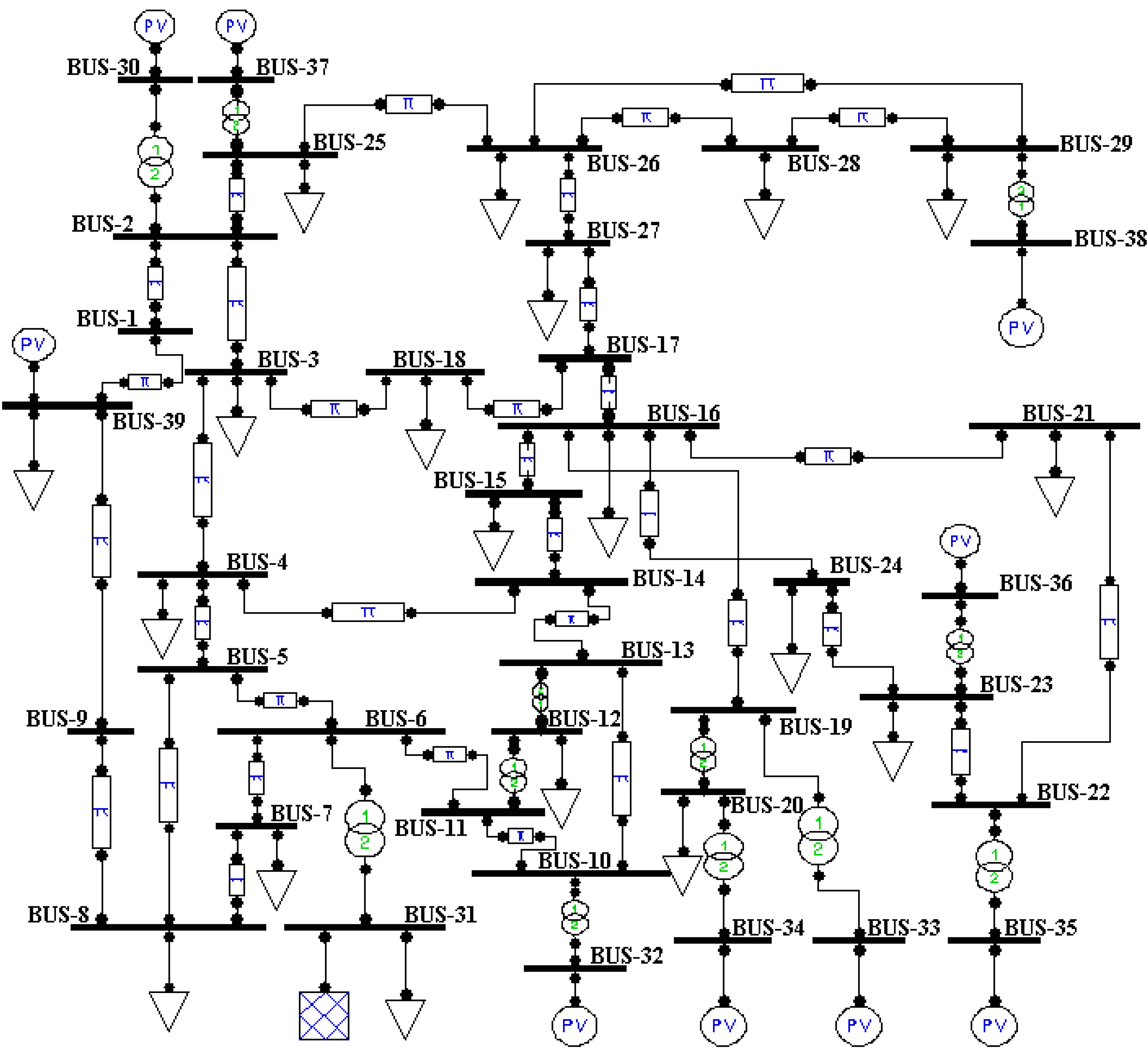
3. Phasor Measurement Unit and Wide Area Measurement System

With the construction of long distance heavily stressed transmission system and the actualization of large scale interconnected power grids, the safety and stability problems of modern power system has become acute, which has also put forward a high requirement for the safety monitoring technology of power network. Based on mature Global Positioning System (GPS) technique and communication technique, Phasor Measurement Unit (PMU) has high stability and reliability, high precision, strong processing, calculating, memorizing and communication capabilities, friendly man-machine interface and openness, it has provided the foundations for dynamic monitoring in electric power system. Under unified time scales, PMU can directly afford the variation curve of voltage, current, phase angle, power, etc. in transient process of power grid, which has also created the conditions for state estimation, on-line security monitoring and dynamic supervising of power grid. On the basis of PMU, Wide Area Measurement System (WAMS) can reflect the dynamic changes of the whole power network in real time. As a new technology and important means which can realize real-time dynamic monitoring in power grid, WAMS has provided a real-time data platform for improving the security and stabilization of power system.
Table 1. The primary technical specifications of Phasor Measurement Unit.
ItemsTechnical Specifications
Sampling for analog inputSampling frequency 4800 Hz, at least 36 channels ,extensible by multiple
GPS timing accuracy1 μ S
Error limit for angle0.01 degree
Error limit for amplitude0.2%(Relative error)
Error limit for power0.5%(Relative error)
Error limit for frequency0.001 Hz, measurement range 45–55 Hz
Dynamic data retained time25 frames/sec, 50 frames/sec, 100 frames/sec
Dynamic data retained time≥14 days
Dynamic data output rate25 frames/sec, 50 frames/sec, 100 frames/sec
Time range for fault recording−5 sec~+15 sec
As to the technical specification of the PMUs, a list of the items in one commercial product of power system real-time dynamic monitoring system is taken as an example and shown in Table 1. The relevant technical details of Wide Area Measurement System and Phasor Measurement Unit can refer to [15,21].
In the research of this paper, the data sources are from Wide Area Measurement System, and they can be gathered by Phasor Measurement Unit, of course, the whole process can be completed by Bonneville Power Administration (BPA) simulations. Thus, the real-time property can be guaranteed by Phasor Measurement Unit and Wide Area Measurement System. Besides, the feature extraction technology of fault coefficient advanced in this paper can be able to extract accurate fault characteristics with high efficiency, and it has strong anti-interference ability and great redundancy.

4. Fault Coefficient Feature Extraction in Complex Electrical Engineering

In order to illustrate the superior feature extraction abilities of fault coefficient feature extraction fundamental, IEEE 39-BUS New England power system will be an experimental subject. The electric diagram of IEEE 39-BUS New England power system is presented in Figure 1. In the network architecture, failures will be discussed in detail. In particular, different levels of Gaussian stochastic interference will be introduced. The anti-interference capability of the fault coefficient feature extraction technology will be deeply analyzed.
Figure 1. IEEE 39-BUS New England power system.
Applsci 05 00307 g001

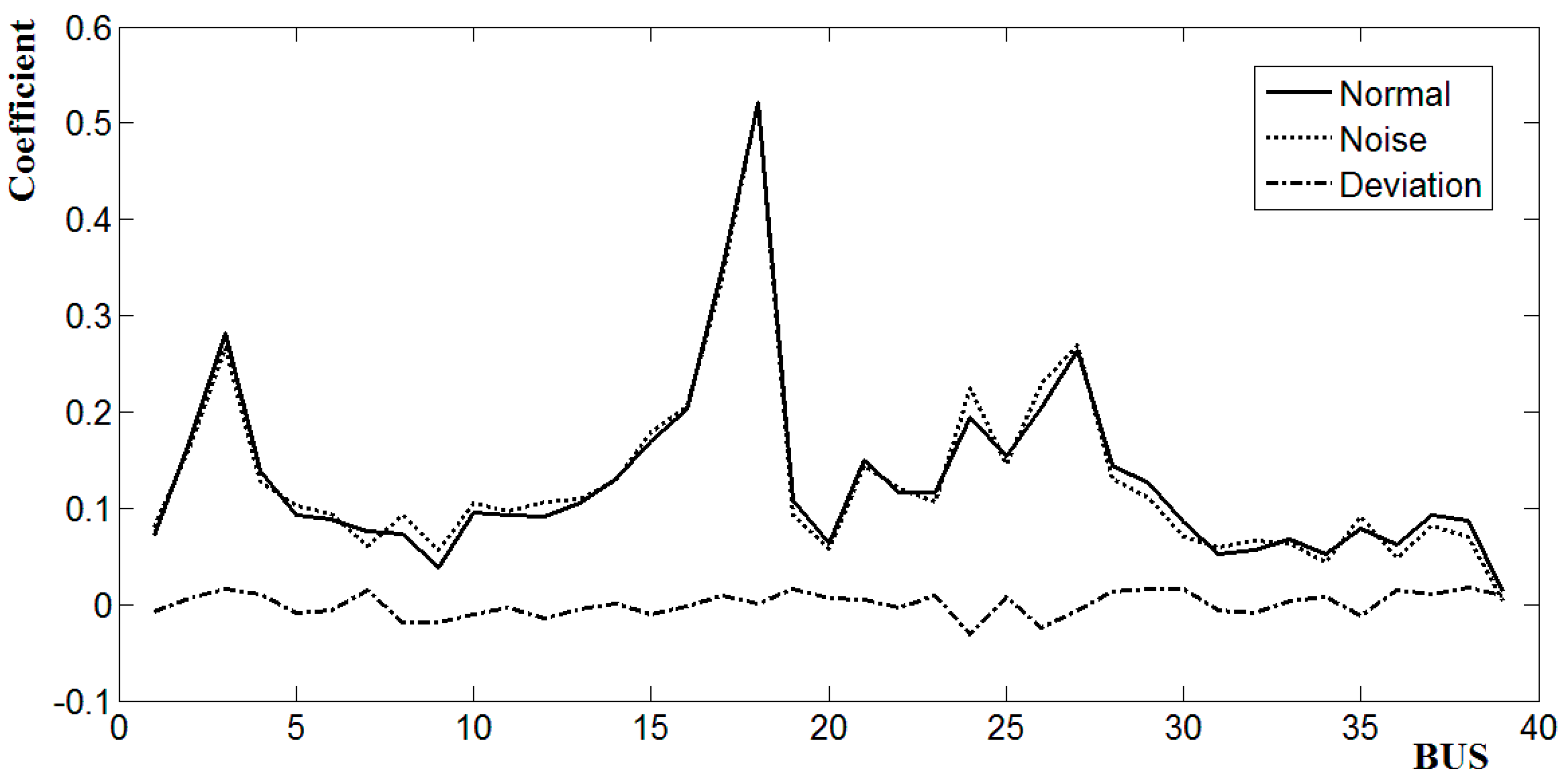
4.1. Fault Coefficient Feature Extraction in Asymmertical Short Circuit Fault

In the IEEE 39-BUS New England power system, an asymmertical short circuit fault breaks out suddenly, and BUS-18 is the actual fault location. By BPA simulations, one can get the node negative sequence voltages. Meanwhile, one has also introduced a white Gaussian stochastic noise N ( 0 , 0.003 2 ) , and carries out detailed analysis about these original electrical information vectors.
According to the fundamental of feature extraction about the fault coefficient, one can calculate the initial characteristic values, initial characteristic vectors, squared loadings and rotation squared loadings. Among them, the initial characteristic value of the first fault factor is 0.01563622, the variance percentage is 0.9852, and the cumulative variance percentage is also 0.9852. For the second fault factor, the initial characteristic value of the first fault factor is 0.00008786, the variance percentage is 0.0056, and the cumulative variance percentage is 0.9908. For the third fault factor, the initial characteristic value of the first fault factor is 0.00007585, the variance percentage is 0.0048, and the cumulative variance percentage is 0.9956. For the fourth fault factor, the initial characteristic value of the first fault factor is 0.00007056, the variance percentage is 0.0044, and the cumulative variance percentage is 1.0000. Actually, only the first fault factor needs to be extracted in this simulation.
Figure 2. The noise influence in asymmertical short circuit fault.
Applsci 05 00307 g002
Furthermore, we calculate the fault coefficient of all fault factors, as shown in Table 2. Because we have focused on the first fault factor, and the general form of the first fault factor is:
Fault 1 = 0.080184BUS1 + 0.162261BUS2 + 0.266219BUS3 + 0.127872BUS4               + 0.101886BUS5 + 0.094243BUS6 + 0.060710BUS7 + 0.092570BUS8               + 0.056463BUS9 + 0.105765BUS10 + 0.096482BUS11 + 0.106159BUS12               + 0.109040BUS13 + 0.128760BUS14 + 0.178810BUS15 + 0.204963BUS16               + 0.337853BUS17 + 0.520984BUS18 + 0.092290BUS19 + 0.057301BUS20               + 0.144469BUS21 + 0.120420BUS22 + 0.106459BUS23 + 0.224937BUS24               + 0.146205BUS25 + 0.228639BUS26 + 0.269287BUS27 + 0.130908BUS28               + 0.110627BUS29 + 0.069968BUS30 + 0.058711BUS31 + 0.065727BUS32               + 0.063605BUS33 + 0.044253BUS34 + 0.091074BUS35 + 0.047710BUS36               + 0.082034BUS37 + 0.069996BUS38 + 0.003890BUS39
In the first fault factor, we will concentrate on the coefficient feature. For all of these coefficients in Fault1, the coefficient of BUS-18 is 0.520984, which is the biggest one. Consequently, we come to the conclusion that BUS-18 is just the fault BUS. In the meantime, the expression of the first fault factor without the interference of white Gaussian stochastic noise has also been obtained through the same approach, namely
Fault 1 = 0.072173BUS1 + 0.168284BUS2 + 0.282617BUS3 + 0.138272BUS4               + 0.092896BUS5 + 0.088251BUS6 + 0.076103BUS7 + 0.073602BUS8               + 0.037873BUS9 + 0.095754BUS10 + 0.093253BUS11 + 0.091824BUS12               + 0.105044BUS13 + 0.130054BUS14 + 0.168642BUS15 + 0.202942BUS16               + 0.347645BUS17 + 0.521645BUS18 + 0.107902BUS19 + 0.063419BUS20               + 0.150062BUS21 + 0.116477BUS22 + 0.115762BUS23 + 0.193652BUS24               + 0.153635BUS25 + 0.204371BUS26 + 0.263681BUS27 + 0.144346BUS28               + 0.126838BUS29 + 0.086465BUS30 + 0.052879BUS31 + 0.056809BUS32               + 0.067171BUS33 + 0.051807BUS34 + 0.078961BUS35 + 0.062526BUS36               + 0.092181BUS37 + 0.087179BUS38 + 0.012862BUS39
In the above expression, the BUS-18 fault certainly has been identified. Let’s further discuss the noise influence for fault coefficients shown in Figure 2. The total average deviation level is 0.00041346. Thus, despite the fact that there is stochastic influence of white Gaussian noise, the fault coefficient feature is still distinct.
Table 2. The fault coefficient in asymmertical short circuit fault.
BUS12345
BUS-10.080184−0.131590−0.1019840.080719−0.003175
BUS-20.1622610.083017−0.250354−0.026744−0.013902
BUS-30.2662190.001688−0.118200−0.064936−0.015069
BUS-40.127872−0.3128570.106917−0.0281920.007209
BUS-50.101886−0.1398610.059463−0.0792730.003251
BUS-60.094243−0.105051−0.0190100.066930−0.004484
BUS-70.0607100.063427−0.0203010.092355−0.011011
BUS-80.0925700.1788990.444781−0.033685−0.011589
BUS-90.0564630.241210−0.0032910.021823−0.015598
BUS-100.105765−0.0196030.252826−0.001555−0.005394
BUS-110.0964820.078763−0.1530920.514546−0.033082
BUS-120.106159−0.291748−0.167308−0.4415530.025298
BUS-130.109040−0.154105−0.1403090.315717−0.014559
BUS-140.1287600.029623−0.2356430.039650−0.012181
BUS-150.1788100.104209−0.050374−0.018207−0.015830
BUS-160.204963−0.2188050.0258840.064883−0.006450
BUS-170.3378530.222826−0.222634−0.000227−0.032912
BUS-180.5209840.0086210.103751−0.109780−0.029657
BUS-190.0922900.0569330.0568480.250654−0.019615
BUS-200.057301−0.102682−0.000145−0.1058310.005540
BUS-210.144469−0.1082410.1507100.117057−0.009449
BUS-220.120420−0.1516390.3261650.254042−0.011526
BUS-230.1064590.019505−0.2077990.109369−0.013268
BUS-240.2249370.0259120.0904120.105611−0.020465
BUS-250.1462050.161939−0.111320−0.011973−0.016714
BUS-260.228639−0.168502−0.098185−0.027499−0.006507
BUS-270.2692870.036244−0.110314−0.081870−0.016063
BUS-280.1309080.0623380.239487−0.136104−0.004834
BUS-290.110627−0.2033510.1762030.087581−0.001551
BUS-300.0699680.010437−0.040059−0.089817−0.001214
BUS-310.058711−0.0274660.051000−0.1651690.004804
BUS-320.0657270.044988−0.0024900.0440750.995845
BUS-330.063605−0.1083940.026131−0.2161390.010330
BUS-340.0442530.2229100.019923−0.096440−0.008673
BUS-350.0910740.4379350.1666880.058293−0.027958
BUS-360.0477100.1136030.083594−0.173864−0.000377
BUS-370.082034−0.1574420.2636790.102439−0.002176
BUS-380.0699960.2872360.128940−0.199584−0.008440
BUS-390.0038900.035845−0.112979−0.0532920.000200

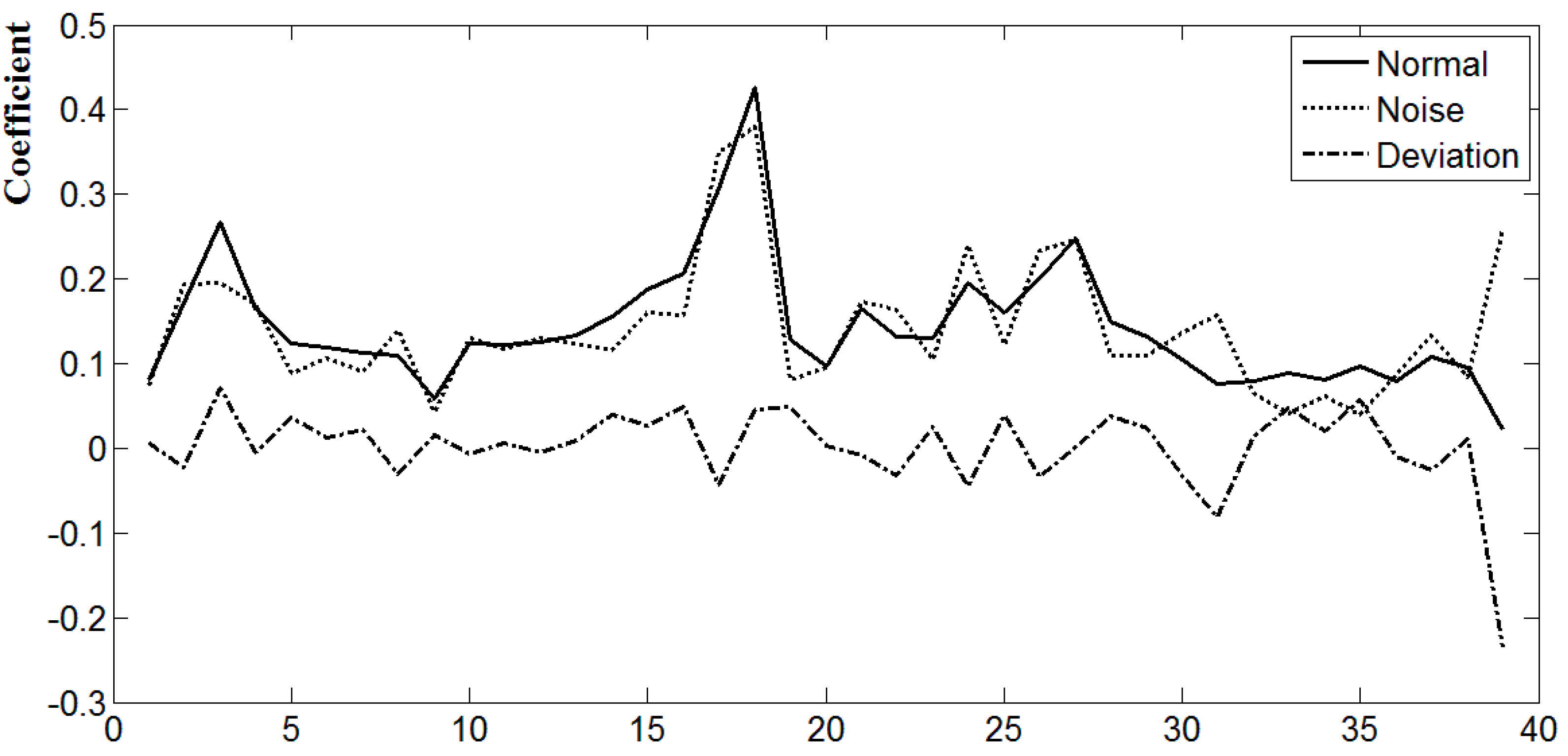
4.2. Fault Coefficient Feature Extraction in Symmetrical Short Circuit Fault

Now, let us further analyze a more complex symmetrical short circuit fault in IEEE 39-BUS New England power system. This time BUS-18 is subjected to a three-phase short circuit fault. By BPA simulations, the node positive sequence voltages have been calculated. In this simulation, let’s introduce a stronger white Gaussian stochastic noise N ( 0 , 0.06 2 ) .
Based on the fundamental of feature extraction about fault coefficient, the initial characteristic values, initial characteristic vectors, squared loadings and rotation squared loadings can also be calculated. Among them, the initial characteristic value of the first fault factor is 1.83004634, the variance percentage is 0.8828, and the cumulative variance percentage is also 0.8828. For the second fault factor, the initial characteristic value of the first fault factor is 0.24305527, the variance percentage is 0.1172, and the cumulative variance percentage is 1.0000. Obviously, the first fault factor is just what we are seeking.
The fault coefficient of all fault factors can be obtained through the same approach (see Table 3). Therefore, the general form of the first fault factor can be written as:
Fault 1 = 0.074346BUS1 + 0.193963BUS2 + 0.195029BUS3 + 0.169430BUS4               + 0.088094BUS5 + 0.106626BUS6 + 0.090224BUS7 + 0.139135BUS8               + 0.042615BUS9 + 0.130098BUS10 + 0.117286BUS11 + 0.130002BUS12               + 0.123483BUS13 + 0.115265BUS14 + 0.160039BUS15 + 0.156472BUS16               + 0.349494BUS17 + 0.380180BUS18 + 0.080870BUS19 + 0.094795BUS20               + 0.173913BUS21 + 0.162841BUS22 + 0.104185BUS23 + 0.239691BUS24               + 0.122016BUS25 + 0.234122BUS26 + 0.245774BUS27 + 0.109912BUS28               + 0.109377BUS29 + 0.137135BUS30 + 0.156919BUS31 + 0.064740BUS32               + 0.041073BUS33 + 0.061483BUS34 + 0.039357BUS35 + 0.087746BUS36               + 0.133753BUS37 + 0.083942BUS38 + 0.258362BUS39
Table 3. The fault coefficient in symmetrical short circuit fault.
BUS12345
BUS-10.0743460.052964−0.001593−0.000682−0.005143
BUS-20.1939630.012428−0.007633−0.007139−0.012111
BUS-30.1950290.039759−0.006921−0.006016−0.012461
BUS-40.169430−0.011105−0.007275−0.007172−0.010351
BUS-50.0880940.1604650.0008140.003357−0.007109
BUS-60.1066260.068563−0.002489−0.001293−0.007299
BUS-70.0902240.073833−0.001669−0.000420−0.006341
BUS-80.139135−0.062473−0.007449−0.008164−0.007946
BUS-90.0426150.0662010.0000780.001137−0.003320
BUS-100.1300980.068635−0.003453−0.002218−0.008750
BUS-110.1172860.075571−0.002734−0.001416−0.008030
BUS-120.1300020.026162−0.004623−0.004025−0.008303
BUS-130.1234830.080095−0.002864−0.001468−0.008460
BUS-140.1152650.027552−0.003978−0.003383−0.007407
BUS-150.1600390.012319−0.006241−0.005803−0.010014
BUS-160.1564720.151342−0.0022500.000264−0.011238
BUS-170.3494940.184110−0.009282−0.005971−0.023503
BUS-180.3801800.074222−0.013582−0.011868−0.024257
BUS-190.080870−0.058891−0.004954−0.005708−0.004384
BUS-200.0947950.064737−0.002108−0.000989−0.006528
BUS-210.1739130.086564−0.004759−0.003186−0.011643
BUS-220.162841−0.009310−0.006954−0.006835−0.009963
BUS-230.104185−0.067407−0.006148−0.006993−0.005736
BUS-240.2396910.013811−0.009475−0.008888−0.014950
BUS-250.1220160.064783−0.003227−0.002063−0.008211
BUS-260.234122−0.000439−0.009640−0.009275−0.014458
BUS-270.245774−0.016099−0.010552−0.010404−0.015015
BUS-280.1099120.2082950.0012390.004533−0.008954
BUS-290.109377−0.027594−0.005261−0.005501−0.006470
BUS-300.137135−0.124739−0.009088−0.010739−0.007175
BUS-310.156919−0.015092−0.006870−0.006848−0.009537
BUS-320.064740−0.166245−0.007259−0.009646−0.002272
BUS-330.041073−0.0276140.9987740.0000000.000000
BUS-340.0614830.010516−0.002238−0.0019830.998048
BUS-350.039357−0.042477−0.0027930.9983180.000000
BUS-360.0877460.1912270.0016790.004682−0.007407
BUS-370.1337530.032855−0.004592−0.003888−0.008604
BUS-380.0839420.085576−0.0010860.000329−0.006075
BUS-390.258362−0.843064−0.033934−0.046151−0.007201
In the first fault factor, the coefficient feature is always crucial. For all of these coefficients in Fault1, the coefficient of BUS-18 is 0.380180, which is also the biggest one. As a result, we come to the conclusion that BUS-18 is the fault BUS. At the same time, the expression of the first fault factor without the interference of white Gaussian stochastic noise can be described:
Fault 1 = 0.080303BUS1 + 0.171509BUS2 + 0.266442BUS3 + 0.165149BUS4               + 0.124600BUS5 + 0.119829BUS6 + 0.112038BUS7 + 0.109471BUS8               + 0.059017BUS9 + 0.124305BUS10 + 0.122919BUS11 + 0.125781BUS12               + 0.133050BUS13 + 0.155540BUS14 + 0.186957BUS15 + 0.205857BUS16               + 0.306195BUS17 + 0.425979BUS18 + 0.129325BUS19 + 0.097090BUS20               + 0.165830BUS21 + 0.131574BUS22 + 0.129598BUS23 + 0.195589BUS24               + 0.161128BUS25 + 0.200178BUS26 + 0.247223BUS27 + 0.148679BUS28               + 0.132369BUS29 + 0.105041BUS30 + 0.075669BUS31 + 0.079530BUS32               + 0.088549BUS33 + 0.081280BUS34 + 0.096113BUS35 + 0.078531BUS36               + 0.108539BUS37 + 0.095568BUS38 + 0.022421BUS39
In the former expression, the real fault location BUS-18 certainly has also been identified. In addition, the noise influence for fault coefficients is presented in Figure 3. In this simulation, the total average deviation level is 0.0016. Therefore, the fault coefficient feature is completely reliable.
Figure 3. The noise influence in symmetrical short circuit fault.
Applsci 05 00307 g003

5. Conclusions

In order to realize real time and accurate fault detection in complex electrical systems, one needs to obtain fault information of electric networks. In the process of power system operation, rich monitoring data includes the system’s normal operation information. Once the fault of a system or equipment occurs, large amounts of fault feature information will be presented, such as operation sequence of protection and circuit breaker recorded by fault recorder, the switching action information, electrical quantities and measuring information provided by the Wide Area Measurement System. All of these have provided data guaranteed for accurate and reliable fault detection.
In this paper, based on the fundamental of feature extraction about the fault coefficient, we have discussed the fault coefficient in complex electrical engineering. According to the research in this paper, the system failure is corresponding to the variable with the biggest coefficient in the first fault factor. For asymmetrical short circuit fault and symmetrical short circuit fault in IEEE 39-BUS New England power system, even if there is strong white Gaussian stochastic interference, the fault coefficient feature is still accurate and reliable. The feature extraction technology about fault coefficient proposed in this paper can extract fault characteristics with high efficiency, and it can satisfy the real-time and accuracy requirements of Wide Area Measurement System and Phasor Measurement Unit. The comparative analysis results of noise influence have also demonstrated the strong anti-interference ability and great redundancy of the fault coefficient feature in complex electrical engineering.

Acknowledgments

The authors thank the earnest and careful anonymous referees for their thoughtful and constructive suggestions that led to a considerable improvement of the paper. This research was supported partly by the National Key Basic Research Project (973 Program) of China (2012CB215200), the NSFC (51277193), the Specialized Research Fund for the Doctoral Program of Higher Education (20110036110003), the Fundamental Research Funds for the Central Universities (2014ZD43) and the Natural Science Foundation of Hebei Province.

Author Contributions

This paper is a result of the full collaboration of all the authors. Yagang Zhang guided the whole research process; Yi Sun wrote Case Study and Methodology; Yinding Wang performed the experiments. All authors discussed the results and commented on the manuscript.

Conflicts of Interest

The authors declare no conflict of interest.

References

  1. Ajami, A.; Daneshvar, M. Data driven approach for fault detection and diagnosis of turbine in thermal power plant using Independent Component Analysis (ICA). Int. J. Electr. Power Energy Syst. 2012, 43, 728–735. [Google Scholar] [CrossRef]
  2. Frank, P.M. Analytical and qualitative model-based fault diagnosis—A survey and some new results. Eur. J. Control 1996, 2, 6–28. [Google Scholar] [CrossRef]
  3. Chakraborty, S.; Keller, E.; Ray, A.; Mayer, J. Detection and estimation of demagnetization faults in permanent magnet synchronous motors. Electr. Power Syst. Res. 2013, 96, 225–236. [Google Scholar] [CrossRef]
  4. Patton, R.J.; Frank, P.M.; Clark, R. Fault Diagnosis in Dynamic Systems Theory and Application; Prentice Hall: Herfordahire, UK, 1989. [Google Scholar]
  5. Frank, P.M. Fault detection in dynamic system using analytical and knowledge-based redundancy—A survey and some new result. Automation 1990, 26, 459–474. [Google Scholar] [CrossRef]
  6. Cho, Y.S.; Jang, G. New technique for enhancing the accuracy of HVDC systems in state estimation. Int. J. Electr. Power Energy Syst. 2014, 54, 658–663. [Google Scholar] [CrossRef]
  7. Korres, G.N.; Tzavellas, A.; Galinas, E. A distributed implementation of multi-area power system state estimation on a cluster of computers. Electr. Power Syst. Res. 2013, 102, 20–32. [Google Scholar] [CrossRef]
  8. Guo, Y.; Wu, W.C.; Zhang, B.M.; Sun, H.B. A method for evaluating the accuracy of power system state estimation results based on correntropy. Int. J. Electr. Power Energy Syst. 2014, 60, 45–52. [Google Scholar] [CrossRef]
  9. Geramifard, O.; Xu, J.X.; Pana, S.K. Fault detection and diagnosis in synchronous motors using hidden Markov model-based semi-nonparametric approach. Eng. Appl. Artif. Intell. 2013, 26, 1919–1929. [Google Scholar] [CrossRef]
  10. Zhang, Y.G.; Wang, Z.P.; Zhang, J.F. Fault identification based on NLPCA in complex electrical engineering. J. Electr. Eng. 2012, 63, 255–260. [Google Scholar] [CrossRef]
  11. Chai, W.; Qiao, J.F. Passive robust fault detection using RBF neural modeling based on set membership identification. Eng. Appl. Artif. Intell. 2014, 28, 1–12. [Google Scholar] [CrossRef]
  12. Zhu, D.; Gao, Q.W.; Sun, D.; Lu, Y.X.; Peng, S.L. A detection method for bearing faults using null space pursuit and S transform. Signal Process. 2014, 96, 80–89. [Google Scholar] [CrossRef]
  13. Zhou, J.; Guo, A.H.; Celler, B.; Su, S. Fault detection and identification spanning multiple processes by integrating PCA with neural network. Appl. Soft Comput. 2014, 14, 4–11. [Google Scholar] [CrossRef]
  14. Harmouche, J.; Delpha, C.; Diallo, D. Incipient fault detection and diagnosis based on Kullback–Leibler divergence using Principal Component Analysis: Part I. Signal Process. 2014, 94, 278–287. [Google Scholar] [CrossRef]
  15. Zhang, Y.G.; Wang, Z.P.; Zhang, J.F.; Ma, J. Fault localization in electrical power systems: A pattern recognition approach. Int. J. Electr. Power Energy Syst. 2011, 33, 791–798. [Google Scholar] [CrossRef]
  16. Zhang, Y.G.; Wang, Z.P.; Zhao, S.Q. BDA fault detection in complex electric power systems. Int. Rev. Electr. Eng. 2012, 7, 3638–3645. [Google Scholar]
  17. Zhang, Y.G.; Wang, Z.P. New fault discrimination under the influence of Rayleigh noise. Adv. Electr. Comput. Eng. 2013, 13, 27–32. [Google Scholar] [CrossRef]
  18. Zhang, Y.G.; Zhao, Z.; Wang, Z.P. Comprehensive detection and isolation of fault in complicated electrical engineering. Electr. Eng. 2013, 19, 31–34. [Google Scholar] [CrossRef]
  19. Wand, X.M. Applied Multivariate Analysis; Shanghai University of Finance and Economics Press: Shanghai, China, 2009. [Google Scholar]
  20. Hair, J.; Joseph, F.; Anderson, R.E.; Tatham, R.L.; Black, W.C. Multivariate Data Analysis; Prentice Hall: Upper Saddle River, NJ, USA, 1998. [Google Scholar]
  21. Martin, K.E.; Benmouyal, G.; Adamiak, M.G.; Begovic, M. IEEE Standard for Synchrophasors for Power Systems. IEEE Trans. Power Deliv. 1998, 13, 73–77. [Google Scholar] [CrossRef]

