2.1. Evolution in Agricultural Land Use and Major Land Allocation Patterns in 1990–2010
This section uses two FAO data sets to examine global land use changes by region to reveal regional common land allocation patterns in response to changes in markets for agricultural commodities. The first set represents expansion and/or contraction in agricultural land (representing changes in cropland cover). In FAO data, pasture is included in cropland, so an expansion in cropland cover indicates deforestation and a reduction in cropland cover could represent reforestation and or conversion of agricultural land to other uses (e.g., expansion in urban areas). The second data set characterizes changes in harvested areas. An expansion in total harvested areas could be due to many factors. The harvested areas of a region may increase due to deforestation (expansion in crop cover), returning idled croplands to crop production, increases in double cropping, or reduction in crop failures. On the other hand total harvested areas may decrease in a region due to reduction in demand for crops, drought or other catastrophic events. In general, over a long time period total harvested area and land cover move together. However in the short run they may diverge. In this section we also use harvested areas to analyze changes in supply of land to alternative crops.
During the time period of 1990–2000 commodity markets were relatively stable, and in many countries agricultural activities were under governmental support programs. The agricultural markets experienced major changes in the next decade. Several countries (in particular, USA and EU members) reduced or modified their agricultural support programs during this decade. Biofuel production began to grow much faster around 2004 in many countries, especially USA, Brazil, and EU. Many counties, especially China and India, observed significant food demand expansion due to rapid economic growth. In addition, the crude oil price reached to its historical high with significant impacts on the production costs of agricultural products. In response to these changes, crop prices went up significantly and agricultural markets experienced major turbulences especially during the years 2008–2011. The higher commodity prices led to increases in cropland cover globally. The study of regional land use changes during these time periods, in particular after 2004, is the key to tuning the land transformation elasticities used in GTAP-BIO model.
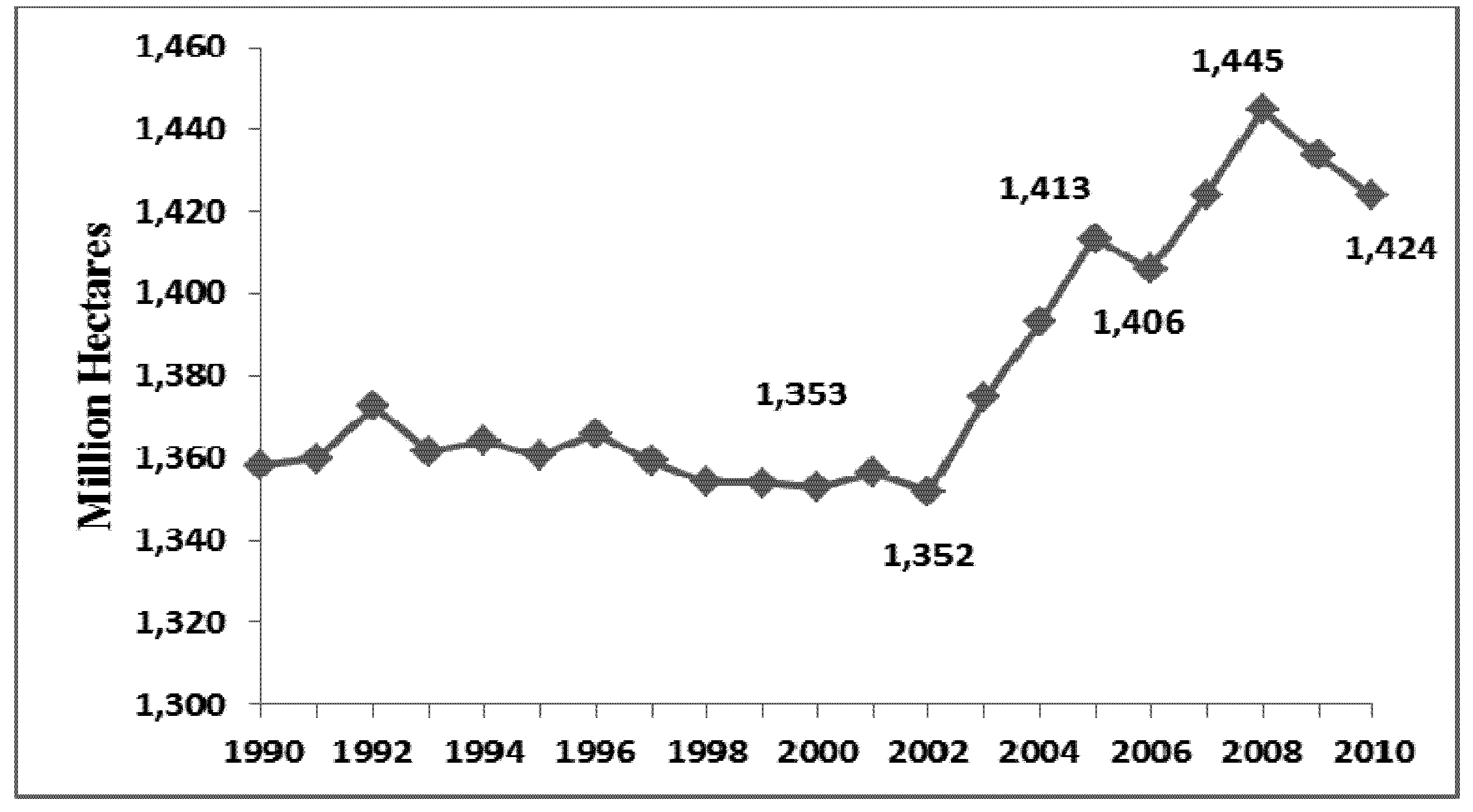
The global area of agricultural land has increased by about 37.5 million hectares (MH) during the past two decades. During this time period the area of global forest has decreased by about 135 MH. These figures confirm land conversion along the land cover frontier at the global scale. On the other hand, the global harvested area followed a relatively flat trend in the 1990s, and then it sharply increased by about 71 MH during the next decades (from 1353 million hectares (MH) in 2000 to about 1424 MH in 2010 (
Figure 2). This rapid growth in the global harvested area reflects major expansion in the demand for agricultural products during the time period 2000–2010.
Figure 2.
Global harvested area 1990–2010.
Figure 2.
Global harvested area 1990–2010.
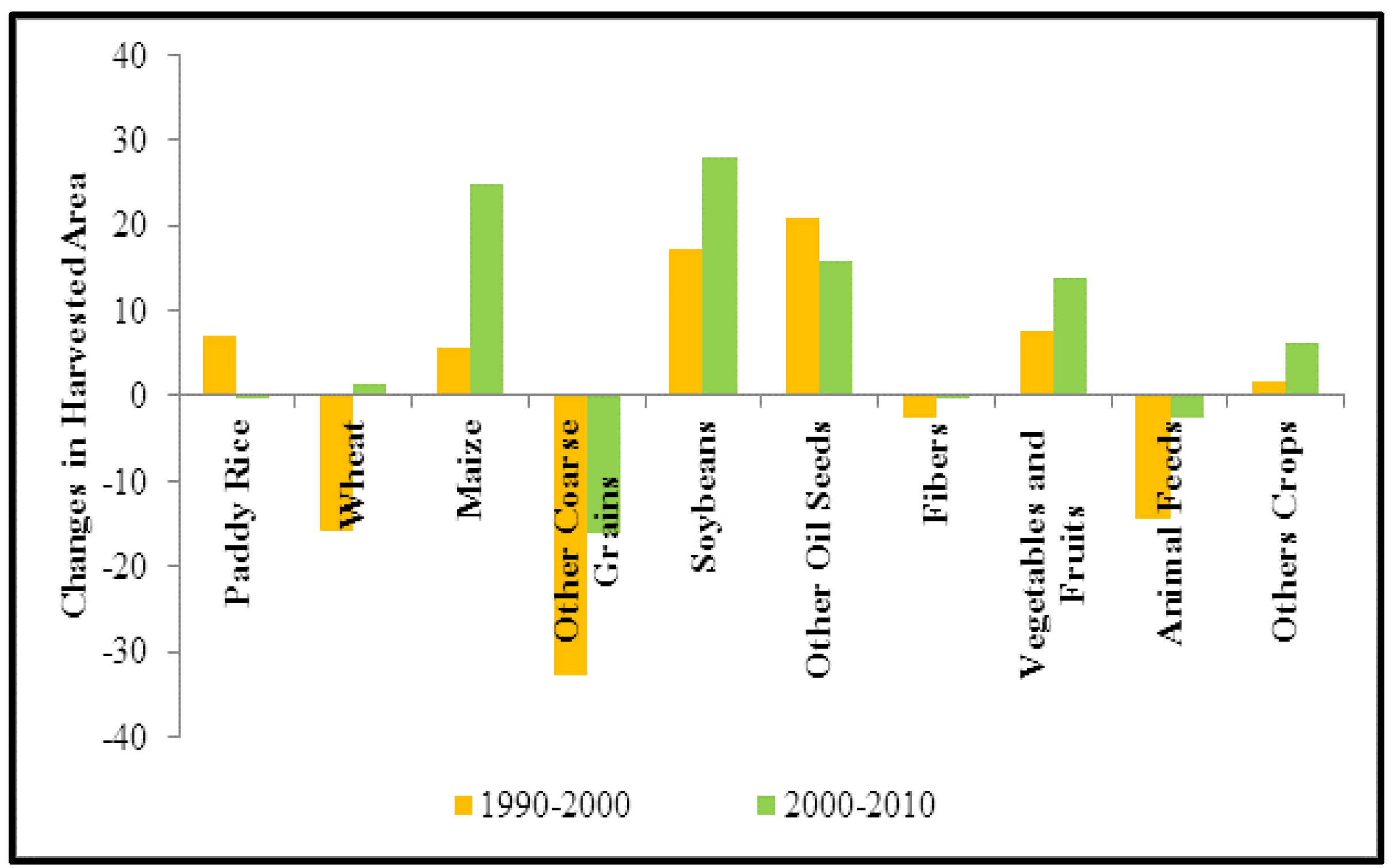
The allocation of cropland among alternative crops has changed significantly during the past two decades.
Figure 3 summarizes changes in global harvested areas by crop for the past two decades (for the list of crop categories and their member see
Table A1 in Appendix A). This figure indicates positive and large changes in the harvested areas of maize and oilseeds and negative and large changes in the harvested areas of crop categories of wheat, other coarse grains, and animal feed. From these observations we can conclude that global harvested area has increased significantly during 2000–2010. However, the rate of land conversion from forest to agricultural land has decreased in this time period compared to the time period of 1990–2000. Reduction in the area of global idled land, increase in double cropping, and reduction in crop failure could help explain the increase in harvested area while forest cover has decreased less.
Figure 3.
Changes in global harvested area by crops (figures are in million hectares).
Figure 3.
Changes in global harvested area by crops (figures are in million hectares).
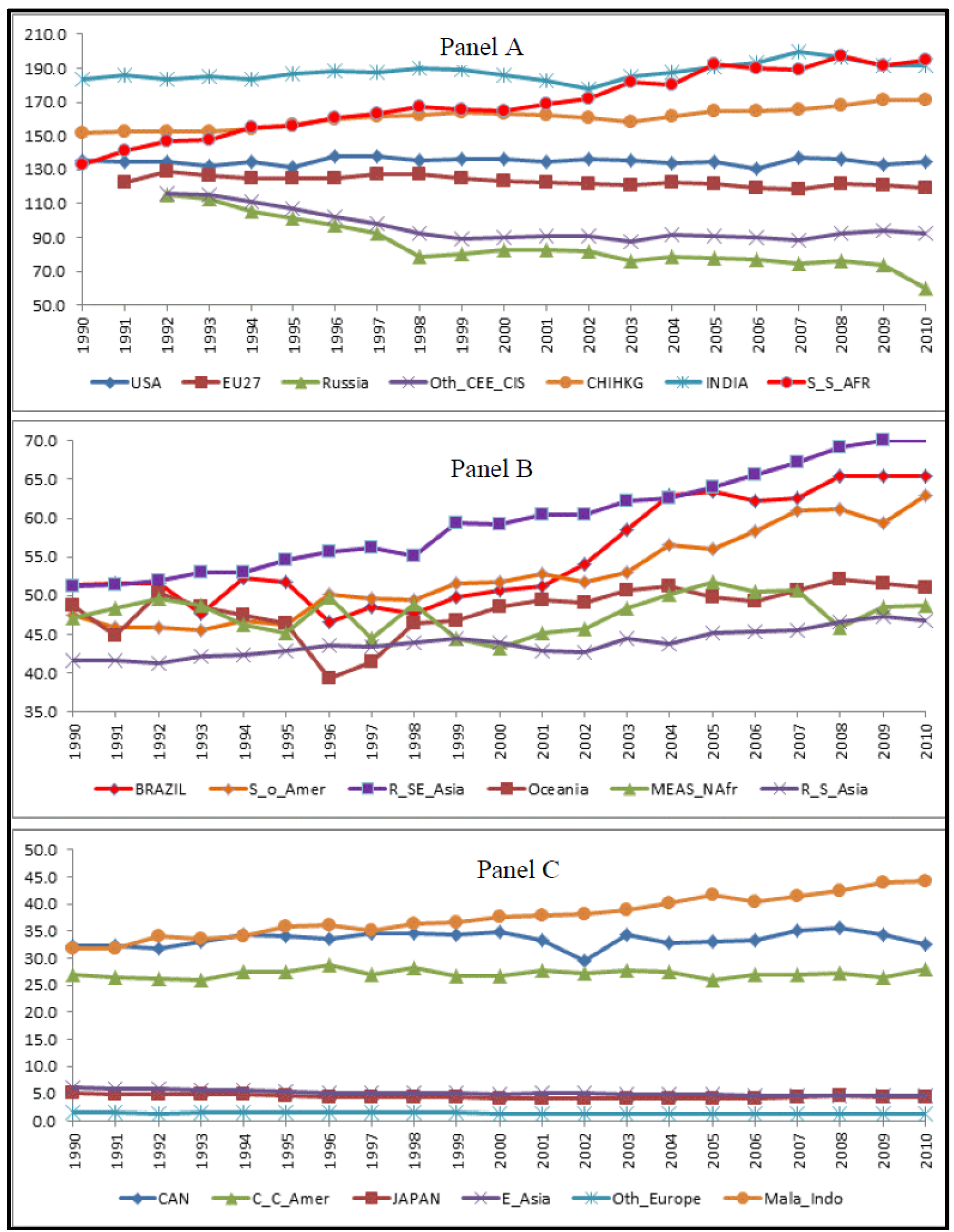
Figure 4.
Global harvested area by region trajectory.
Figure 4.
Global harvested area by region trajectory.
We now examine regional changes in agricultural land and harvested (the regional aggregation is taken from GTAP-GIO model and is presented in
Table B1 in Appendix B).
Figure 4 represents trajectories of harvested areas by region during the past two decades. In general, the 19 regions presented in this figure can be divided into three groups in terms of land conversion among land cover items and among alternative crops.
The first group includes regions or countries for which harvested areas have not changed extensively during the past two decades. However, in these countries allocation of cropland among alternative crops has typically changed over time. For example, during the past two decades the harvested area of USA has remained relatively flat around 135 MH, with minor fluctuations. During this time period (1990–2010) the agricultural land area of this county has decreased by about 5.5%, or about 0.27% per year. Land conversion in this region has happened in favor of reforestation at a small rate (about 0.4 MH per year) during the past two decades. Also, urbanization explains some of the loss in agricultural land. On the other hand, in the USA allocation of cropland among the alternative crops has significantly changed during the past two decades. During this time period the harvested areas of soybeans and maize have increased sharply, while the harvested areas of animal feed crops and wheat have decreased. This indicates that cropland has moved from one crop to another one easily in response to the market forces in the US. Several other countries or regions including EU27, R_S_Asia, and Oth_CES_CIS have followed this pattern.
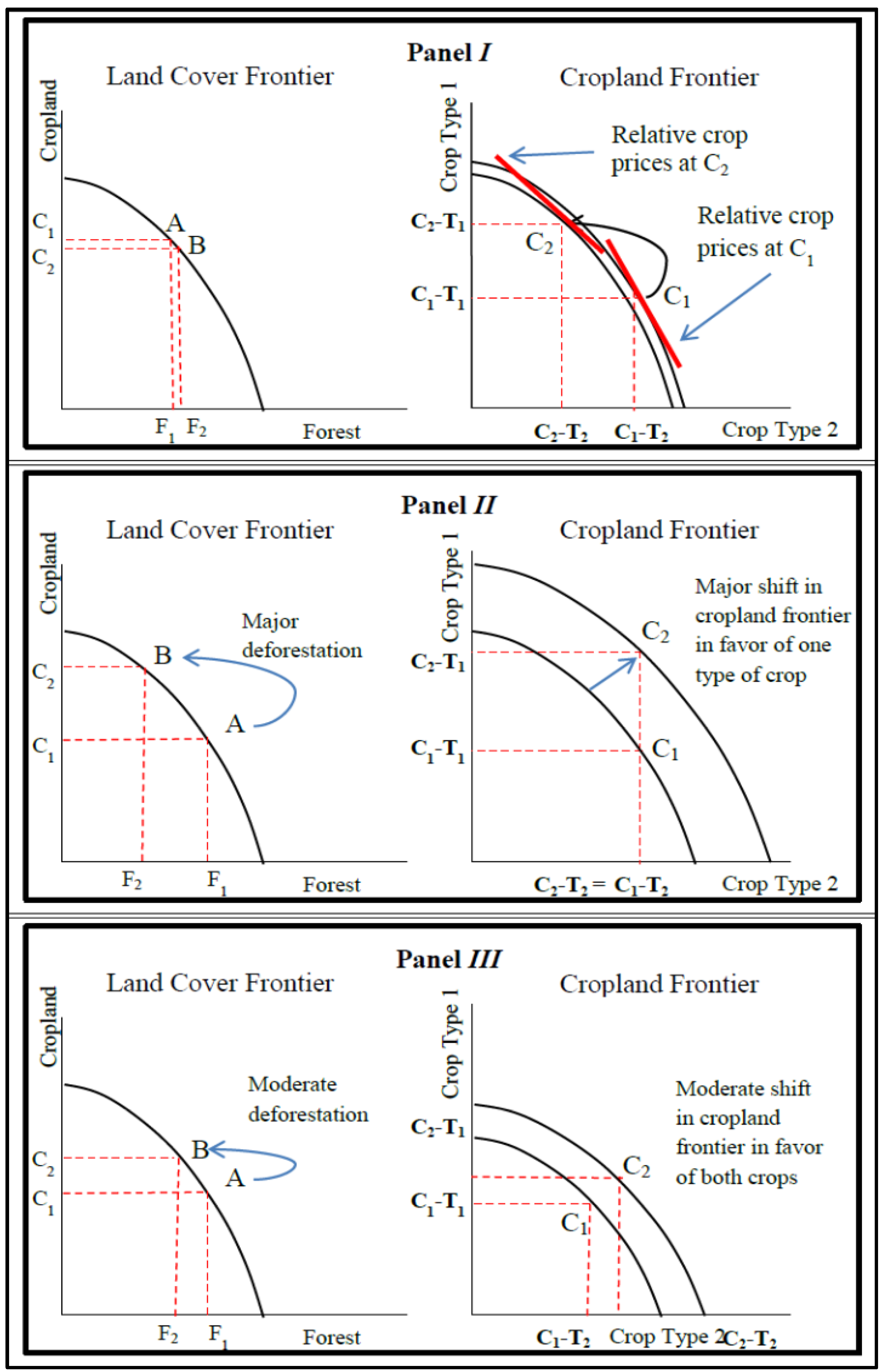
This pattern of land use change can be interpreted as a negligible movement along the land cover frontier and a major move along the cropland frontier as represented in the panel
I of
Figure 5. The left side chart in this panel represents a typical land cover frontier with a small move from agriculture towards forest (which represents the case of USA). This causes an insignificant inward shift in the cropland cover on the right side chart in panel
I. The right hand chart represents a major move along the cropland frontier from crop
type 1 to the crop
type 2 as relative prices of the crops change, represented by the two relative price lines.
The second group represents regions or countries for which harvested area has expanded significantly during the past two decades. For example, the harvested area of Sub Saharan Africa has increased at a rapid rate during the period of 1990–2010, from about 133 MH in 1990 to 165 MH in 2000 and 195 MH in 2010. Hence the harvested area of this region has increased by about 62 MH (46%) during the past two decades. During this time period (1990–2010) the agricultural land area of this region has increased by about 56 MH, and its forest area decreased by 75 MH.
In this region the harvested areas of crop categories of soybeans, animal feed, fiber, wheat, and paddy rice remained constant at their small initial values. However, the harvested areas of crop categories of other oilseeds, vegetable and fruits, other coarse grains (mainly sorghum), maize, and other crops have followed upward trends in 1990s and 2000s. In particular, the harvested areas of vegetable and fruits, other coarse grains, and other oilseeds have increased by 13, 10, and 6.6 MH in 1990s and by 10, 6.4, and 4.3 MH in 2000s.
The observed changes in the harvested area, expansions in agricultural land, and major deforestation in Sub Saharan Africa confirms that in this region a major land conversion has happened from forest to cropland, and the expanded croplands are used to expand production of certain crop categories. This pattern of land use change can be interpreted as large movement along the land cover frontier, for the case of this region in favor of cropland expansion. The expansion in cropland moves the cropland frontier to the right. The panel
II of
Figure 5 which represents a large movement along the land cover frontier demonstrates the pattern of land use changes in this region. Several regions or countries including S_o_America and Mala_Indo have followed this pattern.
Figure 5.
Three patterns of land use changes.
Figure 5.
Three patterns of land use changes.
Finally, consider the third group of countries or regions which fall somewhere in between these polar cases. In this group some countries such as Canada, India, and C_C_Amer observed limited changes in both land cover and cropland frontiers. On the other hand some countries in this group observed land conversions along both frontiers. For example, the harvested area of Brazil has increased by about 14.1 MH during the past two decades. In this country the area of agricultural land has increased by 23 MH and the forest area decreased by about 55 MH in the same time period. These figures show that about 50% of deforestation in Brazil resulted in additions to the cropland area.
The harvested area of soybean has increased from 11.4 MH in 1990 to 13.6 MH in 2000 and 23.3 MH in 2010 in Brazil. The harvested area of maize has frequently fluctuated around 11 to 14 MH during the past two decades. The harvested area of other crops (including sugarcane) followed an upward trend during the past two decades and in particular in 2000s in this country. The harvested area of sugarcane has increased from 4.3 MH in 1990 to 4.8 MH in 2000 and 9.1 MH in 2010. In general, the harvested areas of paddy rice, wheat, fibers, and vegetable and fruits followed downward trends during the time period of 1990 to 2010.
The observed changes in the harvested area and agricultural land in Brazil and changes in the allocation of cropland among crops in this country demonstrate a mix of the first two extreme cases of land use change. This pattern of land use change can be interpreted as a mix of changes along the land cover and cropland frontiers. The panel
III of
Figure 5 which represents movements along the land cover and cropland frontiers demonstrate the pattern of land use changes in this region. Several regions or countries including Japan, E_Asia, and R_SE_Asia, followed this this pattern of land use changes.
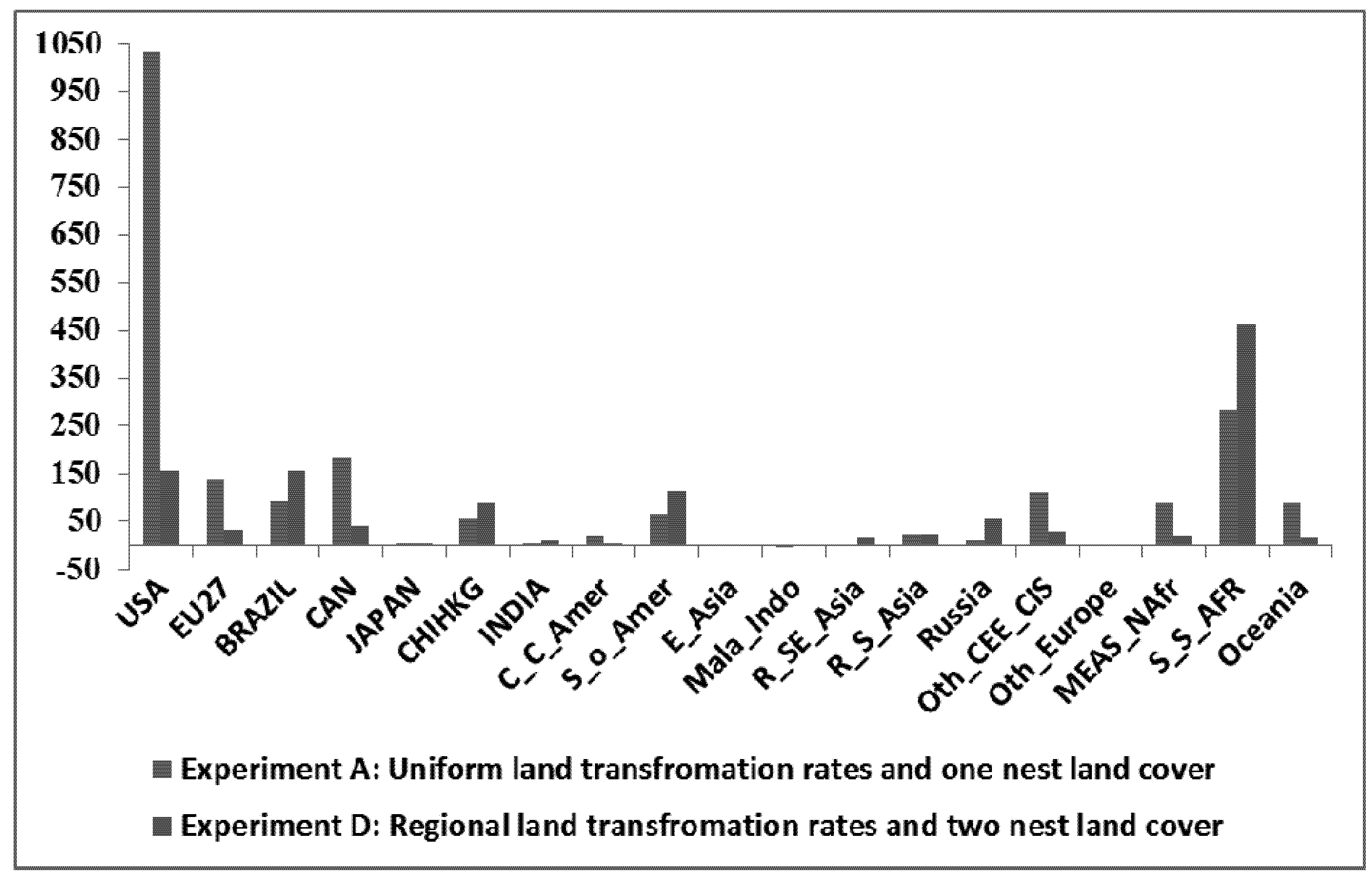
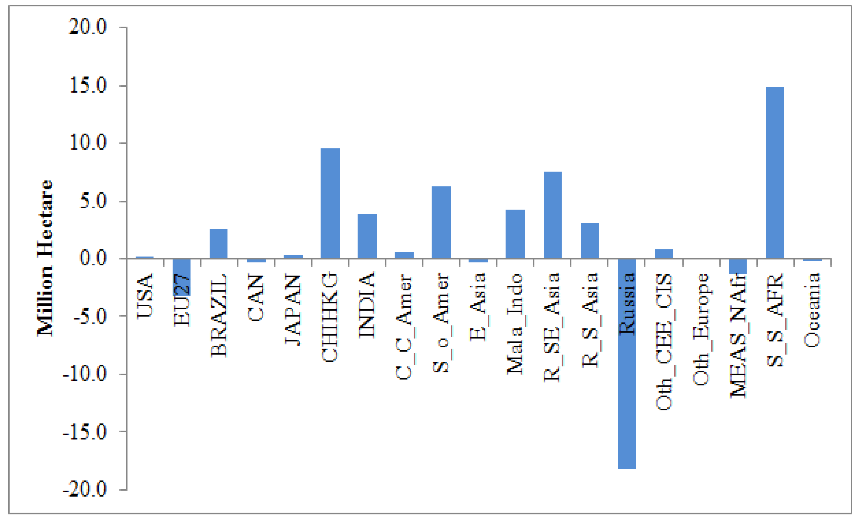
The global harvested area has increased by about 30.6 MH since 2004, when biofuel began to expand rapidly. Several countries such as S_S_Afr, CHIHKG, R_SE_Asia, and S_o_Amer made major contributions to the expansion in global harvested area in this time period. On the other hand, regions such as Russia, EU27, and MEAS_NAfr (Middle East and North Africa) lost a portion of their harvested area since 2004. The reduction in the harvested area of Russia was about 18.1 MH in this time period. A large portion of this reduction was due to crop failure in 2010.
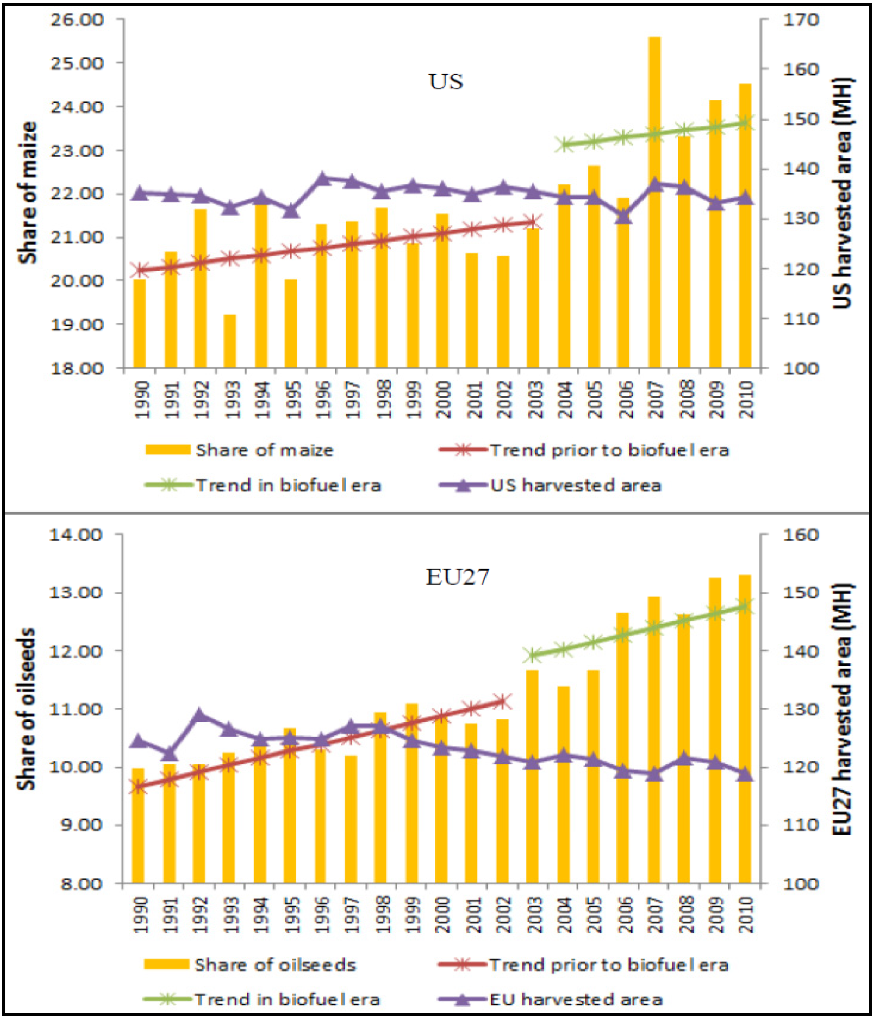
The historical observations confirm that the expansion paths of maize and oilseeds have shifted up in this time period in many regions. For example, the top panel of
Figure 6 summarizes the increasing expansion path of the share of maize in the USA harvested area during the past two decades and in particular since 2004. This graph shows that share of maize in this region has jumped up significantly during the biofuel era. As mentioned earlier, the expansion in maize and soybean harvested areas in the USA caused reductions in harvested areas of other crops and did not lead to expanded cropland area. A similar pattern can be observed in the EU region for the case of biodiesel. The bottom panel of
Figure 6 shows that in this region the expansion in biodiesel production led to a jump in the share of harvested areas of oilseeds, while total harvested area was fluctuating around 120 MH during the biofuel era.
In general since 2004 several countries such as S_S_Afr, CHIHKG, R_SE_Asia, and S_o_Amer made major contributions to the expansion in global harvested area in this time period (
Figure 7). On the other hand, regions such as Russia, EU27, and MEAS_NAfr (Middle East and North Africa) lost a portion of their harvested area since 2004 (
Figure 7). The reduction in the harvested area of Russia was about 18.1 MH in this time period. A large portion of this reduction was due to crop failure in 2010.
Figure 6.
USA and EU27 harvested areas and their oilseeds area share.
Figure 6.
USA and EU27 harvested areas and their oilseeds area share.
Figure 7.
Change in harvested area by region, 2004–2010.
Figure 7.
Change in harvested area by region, 2004–2010.
2.2. Modifications in GTAP Land Transformation Elasticities
This section provides a framework to tune the GTAP land transformation elasticities with the historical observed land used patterns. As mentioned in
section 3 the regional observed trends in land use patterns prior and after the boom in global biofuel industry are very similar, except that the area shares of maize and oilseeds tends to be higher since 2004. For this reason we tune the GTAP land transformation elasticities for the observed patterns during the time period of 2004–2010.
We begin the tuning process with the regional land cover elasticities. The historical changes in total harvested area of a region is a good indication of changes in cropland cover over time, in particular when they are in line with historical changes in forest area. The GTAP-BIO model assumes ETL1 = −0.2 everywhere across the world. As noted in the supporting documents of Hertel
et al. [
7], this relatively small value had been selected from the Ahmed
et al. [
15] calibration process. These authors developed a calibration process to estimate aggregated cropland transformation elasticities as a function of time based on Lubowski [
19] who estimated land supply elasticities for the USA economy using county level data observed in 1982, 1987, 1992, and 1997. Ahmed
et al. [
15] have shown that the land cover transformation elasticity should be small for short to medium run time horizons. The choice ETL = −0.2 is clearly made based on observations on the historical land use changes in USA until 1997. While this figure fairly represents inflexibility in the USA land cover frontier, recent observations confirm more inflexibility in USA land cover frontier at the aggregate level in recent years. For example, recent evidence shows that cropland rent has increased faster than pasture rent in recent years in USA, but the area of cropland remained relatively unchanged. The ratio of cropland rent over pasture rent has increased gradually from about 8 in 2004 to 9.3 in 2010. This means that land owners/farmers had the incentive to move their land from pasture to cropland. However, recent observations indicate that the area of cropland has not increased in the USA in recent years. This confirms a very small land transformation elasticity for the USA land cover frontier.
While data suggest very small land transformation elasticity for US, exiting evidence indicates major movements in land cover in other regions. This means that a uniform and small value of land transformation elasticity does not reflect actual regional observations. To tune this value to the observed changes in land cover of each region, the 19 regions of GTAP-BIO model are ranked based on their absolute value of annual average changes in harvested area since 2004. The results are reported in
Table 1. The 19 regions are divided into four categories based on the following schedule:
Regions with very low rate of land transformation: This category represents regions with very limited changes in land cover during the time period of 2004–2010. The absolute values of changes in the harvested areas of these regions were below 0.25% per year after 2004. To limit land conversion among forest, pasture, and cropland in these regions we assigned a value of ETL1=−0.02 to the lower level of the land supply nest.
Regions with low rate of land transformation: This category represents regions with relatively low annual rates of land transformation during the targeted time period. The absolute value of changes in the harvested areas of these region where higher than 0.25% and lower than 0.75% since 2004. For these regions we assigned a value of ETL1=−0.1 (half of the original value of GTAP-BIO model) to the lower level of their land supply nest.
Regions with high rate of land transformation: This group represents regions with relatively large changes in their harvested areas. The absolute values of changes in the harvested areas of these regions were larger than 0.75% and less than 1.5% per year since 2004. To facilitate land conversion among forest, pasture, and cropland in these regions we assigned a value of ETL1=−0.2 (the original value of GTAP-BIO model) to the lower level of the land supply nest.
Regions with very high rate of land transformation: The last category includes regions with high very high rates of land transformation. The absolute values of changes in the harvested areas of these regions were larger than 1.5% per year during the targeted time period. A relatively high value of ETL1=−0.3 is assigned to the lower level of land supply tree of these regions.
Table 1.
Tuned regional land transformation elasticities.
Table 1.
Tuned regional land transformation elasticities.
| Regions | Absolute value of annual changes in harvested area (%) | Rank in land cover change | Tuned ETL1 | Tuned ETL2 |
|---|
| Oth_Europe | 0.06 | Very Low | −0.02 | −0.25 |
| Oceania | 0.09 | −0.02 | −0.25 |
| CAN | 0.10 | −0.02 | −0.25 |
| USA | 0.10 | −0.02 | −0.75 |
| MEAS_NAfr | 0.11 | −0.02 | −0.25 |
| Oth_CEE_CIS | 0.14 | −0.02 | −0.75 |
| C_C_Amer | 0.17 | −0.02 | −0.25 |
| EU27 | 0.22 | −0.02 | −0.75 |
| INDIA | 0.49 | Low | −0.1 | −0.25 |
| R_S_Asia | 0.73 | −0.1 | −0.25 |
| Russia | 1.00 | High | −0.2 | −0.75 |
| JAPAN | 1.09 | −0.2 | −0.5 |
| CHIHKG | 1.10 | −0.2 | −0.25 |
| E_Asia | 1.11 | −0.2 | −0.5 |
| BRAZIL | 1.54 | Very High | −0.3 | −0.5 |
| R_SE_Asia | 1.68 | −0.3 | −0.5 |
| Mala_Indo | 1.82 | −0.3 | −0.25 |
| S_o_Amer | 2.37 | −0.3 | −0.25 |
| S_S_AFR | 2.50 | −0.3 | −0.5 |
We now turn to land transformation elasticity among crops. To tune this elasticity with historical observations all crop categories are collapsed into two groups. The first group covers maize and oilseeds and is named MO. The second group represents all other crop types and named OC. During the past decades and in particular since 2004 global demands for MO crops have increased significantly. The historical observations indicate that in response to the higher demands for MO crops several countries have shifted their cropland to produce these crops, some countries expanded their cropland to increase their MO production, and some other countries made no major changes in their land allocation in response to the changes in global market for these crops. To assess the flexibility of countries in their cropland frontier we rely on the regional changes in the harvested areas of MO and OC crops.
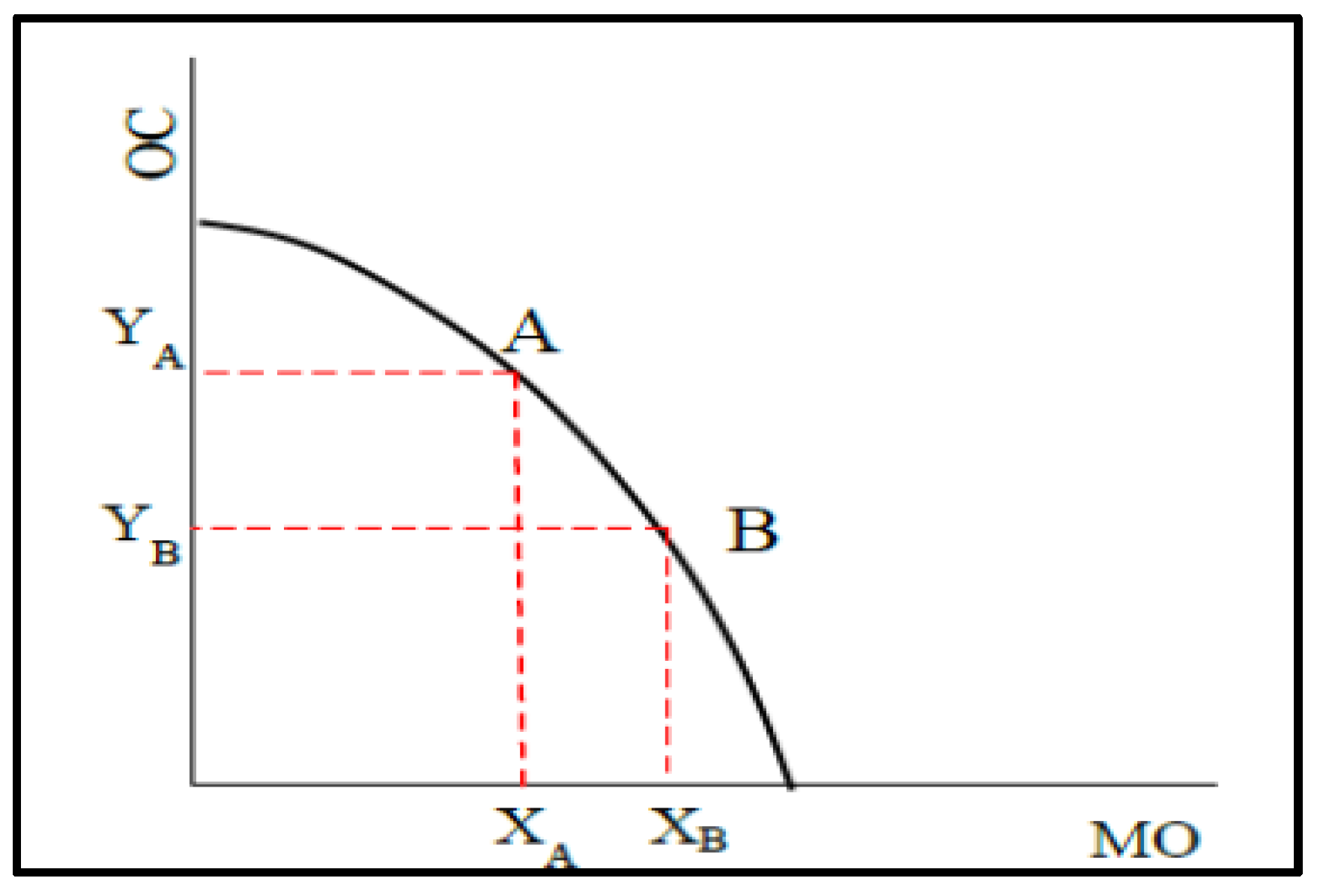
To establish a benchmark consider the USA economy which shifted a big portion of its existing cropland to produce more
MO crops without expansion in its cropland area during the past two decades and in particular since 2004. It is straight forward to evaluate the cropland transformation elasticity for this economy using the concept of Arch Transformation Elasticity (ATE). To establish the theoretical base consider
Figure 8 which represents moving over the cropland frontier from point
A to point
B to produce more
MO crops. For this movement the size of ATE can be obtained from the following relationship
![Applsci 03 00014 i001]()
. For example, suppose point
A represents the year 2003 (one year before biofuel boom) and point B represents 2010. Then ATE = −0.86 for the USA economy between 2003 and 2010. If we change the base to 2002 then ATE = −0.76 and if we change the end year to 2009 then ATE = −0.67. Note that in calculating these values we dropped the term
![Applsci 03 00014 i002]()
from the above formula because
XB were equal
YB in recent years. All of these numbers are indeed around ETL2 = −0.75 used in the latest versions of GTAP-BIO developed by Taheripour
et al. [
17] and Tyner
et al. [
18]. We considered this value of ETL2 as the highest rate of land transformation for the cropland cover. The cropland transformation elasticities of other regions are tuned with respect to this benchmark. To accomplish this task the same high value of −0.75 is assigned to the ETL2 for EU, Russia, and Oth_CEE_CIS regions, which observed limited or no expansion in their cropland and moved their existing cropland to
MO crops since 2004. On the other hand, for those regions which experienced no major expansion in their cropland area and had no significant changes in their land allocation among crops, we assigned a low value of −0.25 to their ETL2 rate. Several regions including Canada, C_C_Amer, Oth_Europe, MEAS_NAfr, and Oceania fall in this group.
Figure 8.
Moving towards MO crop without cropland expansion.
Figure 8.
Moving towards MO crop without cropland expansion.
Finally, a test is developed to decide about the size of ETL2 for other countries which experienced expansion in their cropland and observed changes in their cropland allocation among the
MO and
OC crops. The test which is explained in Appendix C determines the sources of changes in the area of
MO crops in each region over time. The area of
MO crop in each region could change due to two sources. It can change either due to expansion in cropland or a combination of expansion in cropland and switching from production of
OC to
MO crops. In each region, if the expansion occurred only due to cropland expansion, then a limited value of −0.25 is assigned to ETL2 of that region, otherwise a value of −0.5 is used. A full set of new regional ETL2 is presented in
Table 1.
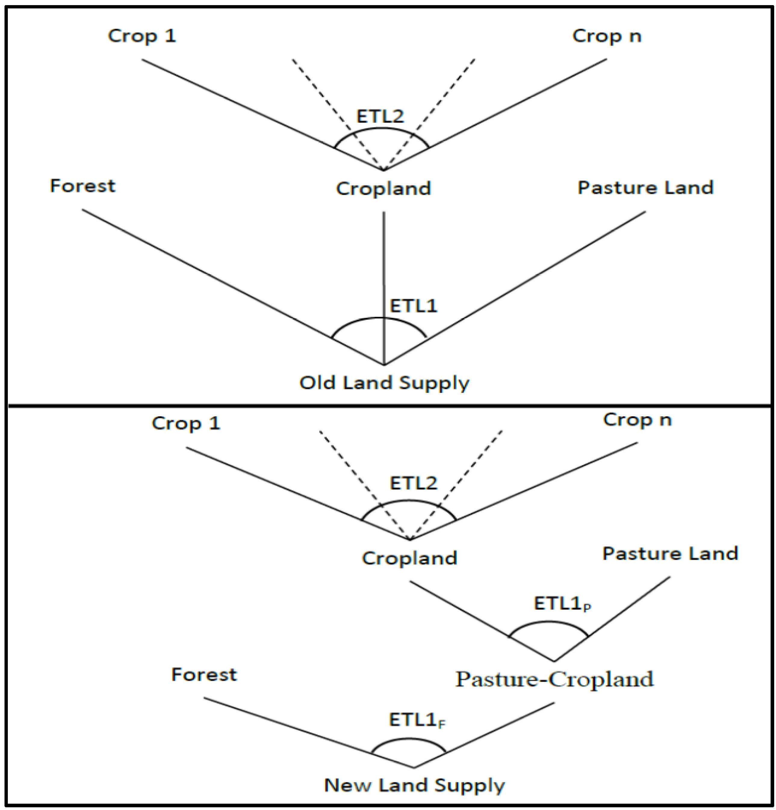
2.3. Change in the Land Cover Nesting Structure
The GTAP-BIO model divides the managed land cover of each region into three broad land categories of cropland, forest, and pasture by AEZ. Cropland denotes existing cultivated land. Managed forest represents all types of forests, and pastureland covers all types of range, grassland, and pasture. Pasture does not include shrubland, which cannot be converted to cropland in GTAP. In this model land can move from one type to another type subject to economic and biophysical constraints. For example, a low productivity pasture will not be converted to cropland when a more suitable land is available for conversion. The supply of and demand for land are modeled at the AEZ level. The derived demands for cropland, forest and pasture are determined from the production functions of crop, forest, and livestock sectors. The land supply side of the model represents a land allocation CET process. The implemented land supply structure of the earlier versions of the GTAP-BIO model put forest, pasture, and cropland in one nest and assumed that forest and pasture land can be converted to crop land with identical rates of land transformation elasticities. This implies that land can be converted from forest and pasture to cropland with equal ease and/or economic opportunity cost. In the real world often it is not as easy or inexpensive to convert forest to cropland as pasture. For example, farmers frequently switch back and forth from pasture and grassland to crop production and
vice versa in the Northern Plains regions of the USA (including parts of Iowa, Minnesota, North Dakota, South Dakota and Montana) [
20] where converting grasslands to crop production and
vice versa is not costly. However, transforming managed forests to cropland is not a common practice. In general, per hectare cost of converting one type of land to another type is equal to the difference in their present values per hectare [
21], the value of each type of land is equal to the net present value of its future annual net return/rent, and the net present value of land can evaluated by its annual rent over a discount rate. Gurgel
et al. [
21] have shown that in general pasture land rent is higher than forest land rent, and both of these land rents are smaller than cropland rent across the world except in a few places. This means that the net costs of converting pasture land to crop production should be less than the net costs of converting forest to cropland. Putting forest, pasture, and cropland in the same nest ignores this important fact.
To remove this deficiency, we created a new land supply nesting structure, shown in the bottom panel of
Figure 1, which has cropland and pasture in one nest and the substitution between forest and the combined “
pasture–cropland” in the second nest. In this paper we use the notation “
pasture–cropland” for the combination of pasture and cropland in the land supply tree. We continue to use the notation “cropland pasture” for low productivity cropland which has been cultivated in past but is not under crop production at present. In the new nesting structure parameter ETL1
F shows the land transformation rate between forest and combined pasture–cropland, parameter ETL1
P indicates the land transformation rate between cropland and pasture land, and parameter ETL2 represents the rate of land transformation among cropping activities as usual.
To take into account the fact that converting pasture land to cropland is easier and/or less costly than converting forest to cropland, it is assumed that in each region the value of ETL1
P is α percent larger than the value of ETL1
F. Note that, in the absolute term, the higher the value of land transformation elasticity the lower the economic cost of land transformation. In addition, to preserve the tuned regional ETL1 values presented in
Table 1, it is assumed that in each region values of ETL1
F and ETL1
P deviate from the value of ETL1 of that region by plus and minus β, respectively. Under these assumptions it is straight forward to show that: β= α/(200 + α). In this paper we assumed that ETL1
P is 20% larger than ETL1
F to take into account the fact that converting forest to cropland is more costly than converting pasture land to cropland. Given these assumptions the regional values for ETL1
F and ETL1
P are obtained from the regional values of ETL1 presented in
Table 1. The calculated values for these land transformation values are presented in
Table 2.
Table 2.
Tuned regional land cover transformation elasticities.
Table 2.
Tuned regional land cover transformation elasticities.
| Regions | Rank in land cover change | Tuned ETL1 | Tuned ETL1F | Tuned ETL1P | Tuned ETL2 |
|---|
| Oth_Europe | Very Low | −0.02 | −0.018 | −0.0218 | −0.25 |
| Oceania | −0.02 | −0.018 | −0.0218 | −0.25 |
| CAN | −0.02 | −0.018 | −0.0218 | −0.25 |
| USA | −0.02 | −0.018 | −0.0218 | −0.75 |
| MEAS_NAfr | −0.02 | −0.018 | −0.0218 | −0.25 |
| Oth_CEE_CIS | −0.02 | −0.018 | −0.0218 | −0.75 |
| C_C_Amer | −0.02 | −0.018 | −0.0218 | −0.25 |
| EU27 | −0.02 | −0.018 | −0.0218 | −0.75 |
| INDIA | Low | −0.1 | −0.0909 | −0.1091 | −0.25 |
| R_S_Asia | −0.1 | −0.0909 | −0.1091 | −0.25 |
| Russia | High | −0.2 | −0.1818 | −0.2182 | −0.75 |
| JAPAN | −0.2 | −0.1818 | −0.2182 | −0.5 |
| CHIHKG | −0.2 | −0.1818 | −0.2182 | −0.25 |
| E_Asia | −0.2 | −0.1818 | −0.2182 | −0.5 |
| BRAZIL | Very High | −0.3 | −0.2727 | −0.3273 | −0.5 |
| R_SE_Asia | −0.3 | −0.2727 | −0.3273 | −0.5 |
| Mala_Indo | −0.3 | −0.2727 | −0.3273 | −0.25 |
| S_o_Amer | −0.3 | −0.2727 | −0.3273 | −0.25 |
| S_S_AFR | −0.3 | −0.2727 | −0.3273 | −0.5 |


 . For example, suppose point A represents the year 2003 (one year before biofuel boom) and point B represents 2010. Then ATE = −0.86 for the USA economy between 2003 and 2010. If we change the base to 2002 then ATE = −0.76 and if we change the end year to 2009 then ATE = −0.67. Note that in calculating these values we dropped the term
  from the above formula because XB were equal YB in recent years. All of these numbers are indeed around ETL2 = −0.75 used in the latest versions of GTAP-BIO developed by Taheripour et al. [17] and Tyner et al. [18]. We considered this value of ETL2 as the highest rate of land transformation for the cropland cover. The cropland transformation elasticities of other regions are tuned with respect to this benchmark. To accomplish this task the same high value of −0.75 is assigned to the ETL2 for EU, Russia, and Oth_CEE_CIS regions, which observed limited or no expansion in their cropland and moved their existing cropland to MO crops since 2004. On the other hand, for those regions which experienced no major expansion in their cropland area and had no significant changes in their land allocation among crops, we assigned a low value of −0.25 to their ETL2 rate. Several regions including Canada, C_C_Amer, Oth_Europe, MEAS_NAfr, and Oceania fall in this group.