
Asphalt Pavement Transverse Cracking Detection Based on Vehicle Dynamic Response

1
School of Civil and Transportation Engineering, Ningbo University of Technology, Ningbo 315211, China
2
The Key Laboratory of Road and Traffic Engineering, Ministry of Education, Tongji University, Shanghai 201804, China
*
Author to whom correspondence should be addressed.
Appl. Sci. 2023, 13(22), 12527; https://doi.org/10.3390/app132212527
Submission received: 8 October 2023
/
Revised: 12 November 2023
/
Accepted: 19 November 2023
/
Published: 20 November 2023
(This article belongs to the Topic Advances in Non-Destructive Testing Methods, 2nd Volume)
Abstract
:Featured Application
This paper proposes a novel method for transverse cracking detection based on vehicle vibration response.
Abstract
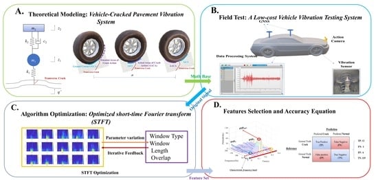
Transverse cracking is thought of as the typical distress of asphalt pavements. A faster detection technique can provide pavement performance information for maintenance administrations. This paper proposes a novel vehicle-vibration-based method for transverse cracking detection. A theoretical model of a vehicle-cracked pavement vibration system was constructed using the d’Alembert principle. A testing system installed with a vibration sensor was put in and applied to a testing road. Then, parameter optimization of the Short-time Fourier transform (STFT) was conducted. Transverse cracking and normal sections were processed by the optimized STFT algorithm, generating two ideal indicators. The maximum power spectral density and the relative power spectral density, which were extracted from 3D time–frequency maps, performed well. It was found that the power spectral density caused by transverse cracks was above 100 dB/Hz. The power spectral density at normal sections was below 80 dB/Hz. The distribution of the power spectral density for the cracked sections is more discrete than for normal sections. The classification model based on the above two indicators had an accuracy, true positive rate, and false positive rate of 94.96%, 92.86%, and 4.80%, respectively. The proposed vehicle-vibration-based method is capable of accurately detecting pavement transverse cracking.
1. Introduction
Pavement distress detection is significant for road maintenance [1]. Transverse cracking is a typical form of distress that indicates asphalt pavement surface or base damage [2]. If transverse cracking cannot be repaired in time, it will deteriorate pavement strength, stiffness, and durability [3]. Furthermore, the whole transportation system cannot operate smoothly and safely. Therefore, it is vital for highway maintenance departments to detect transverse cracking efficiently and effectively.
Traditional detection methods for pavement distress include manual-based and image-based techniques. The manual-based method plays an important role in low-grade highway distress detection. This method can detect all types of distress. At the same time, its detection efficiency and accuracy remain low. However, data reprocessing of the manual-based method is highly subjective, complex, and does not fit the needs of large-scale road network detection [4]. Due to the above problems, automatic detection based on images has been proposed and applied widely [5]. Compared with the manual-based method, its detection efficiency is superior. However, its accuracy depends on features generated through a manual process or machine learning algorithm [6]. The automatic method mainly refers to an image-based method, which needs to be trained using other methods, such as deep learning, reinforcement learning, etc. [2,5,6]. In general, if maintenance departments expect to obtain timely pavement distress information of a huge traffic network, an image-based method cannot fulfil this expectation.
In recent years, indirect damage detection of traffic infrastructure using a moving test vehicle has gradually risen [7]. Yang and co-workers first proposed extracting bridge frequencies from a moving test vehicle’s dynamic response [8]. Compared with the direct method for setting vibration sensors on the traffic infrastructure, the indirect approach is generally less costly, less risky, and less laborious [9].
However, pavement distress detection based on a vehicle’s dynamic response is still in developmental stages. Yu and co-workers proposed that the mechanical response of automobile vibrations can be used to detect pavement distress. The vibration response’s magnitude and frequency depend on the severity of the pavement distress, including cracks and surface rutting [10]. The MIT Laboratory of Computing and Artificial Intelligence proposed a P2 road monitoring architecture for pothole detection. During field testing, over 90% of the identified potholes needed maintenance [11]. In addition, smartphone-based vibration sensing has become a significant technique for detecting road surface conditions [12]. Nericell is a system for the monitoring of road conditions through mobile smartphones equipped with some sensors. These conditions include bumps, potholes, braking, and honking [13]. Wolverine is another typical traffic and road condition estimation system using smartphone sensors that collects acceleration in three directions. More importantly, the system adopts a machine learning method (SVM) to improve its false negative rates [14]. However, the smartphone sensing method has lower accuracy, especially in transverse cracking detection. Qun Yang and his co-workers focused on identifying transverse cracking of asphalt pavement through professional vibration sensors. Their study included the time, frequency, wavelet, and statistical analysis of the vehicle vibration signal [15]. Six main features were extracted from different domains, which generated eight classification models, and the feasibility of this method was investigated using 2292 pavement sections [6]. Bruno S’s team focus on monitoring the road network through a low-cost system based on vehicle vibration, which reached the ideal effects for evaluating the pavement conditions [16,17,18]. Apart from that, some excellent dynamic vehicle models have been established to illustrate the basic principle between the pavement condition and the vehicle [19].
Most studies concentrate more on time or frequency domain analysis. The features extracted from the time or frequency domain are better when passing by some obvious distress, such as potholes and rutting. However, the features caused by transverse cracking are limited in the time or frequency domain, making them hard to detect. Pavement transverse cracking hardly affects the threshold of vehicle acceleration amplitude because of its limited length along the driving direction. Similarly, the Fourier transform just reflects the whole frequency distribution of the vehicle’s vibration signal. It is challenging to express small signal mutations caused by transverse cracking, including its location. Apart from that, vehicle parameters are also important. Different locations can generate different dynamic responses. Different vehicle types, including fuel-driven and electric-driven, also affect the response amplitude [20]. So, it is necessary to select the right car and the ideal response location [21].
Consequently, the present work aims to accurately identify pavement transverse cracking damage using a vehicle dynamic response. To that end, this paper formulates a novel strategy to explore time–frequency features using a Short-time Fourier transform (STFT) and better characterization indicators. More importantly, this novel method can balance the key points, including detection accuracy, equipment cost, and efficiency. The detection method based on a vehicle’s dynamics response solves the problems of low detection frequency and the high cost of existing detection methods. Through the optimized STFT algorithm, the method overcomes the lack of detection accuracy caused by traditional time-domain analysis or frequency-domain analysis. This is because the optimized STFT algorithm focuses more on transverse cracking detection, which takes into account the accuracies of both time- and frequency-domain information recognition.
2. Theoretical Modeling
Suppose the vertical displacement between the wheel and the body is Z1 and Z2, respectively. The coordinate origin is the equilibrium position between the wheel and the body, shown in Figure 1. m1 and m2 denote the quality of the wheel and body, respectively. k1 and k2 denote the stiffness of the tire and spring, and c2 denotes the damping coefficient of the shock absorber. In this study, we see the tire as an undamped linear spring system.
For a quarter vehicle-normal pavement system, the equation of motion is constructed based on the d’Alembert principle [22], which is shown in Equations (1) and (2):
where the first-order derivation of the vertical displacement denotes the vertical speed and the second-order derivation of the vertical displacement indicates the vertical acceleration.
The equation of motion for a quarter vehicle-cracked pavement system is constructed following Equations (3) and (4).
In Equations (2) and (4), the system’s input is expressed as q (normal pavement) and q’ (cracked pavement), which denotes the pavement’s surface profile. They can be represented in the complex exponential form:
where ω denotes angular frequency, and q0 is the initial profile. δ denotes the transient impulse caused by transverse cracking, which is affected by the crack’s cracking degree. Δt is the response time that the wheel passes by the transverse crack.
The tire-cracked pavement contact process is shown in Figure 2a. During actual driving, the tire and the pavement are always in contact with a certain geometry, defined as ground contact (GC). In addition, the contact shape between transverse cracking and the tire is not a point but a certain geometric area, defined as the Areas of Crack Action (ACA).
The cracks are located at the junction of the ground surface (GC1) and the action surface when first touching the transverse cracked pavement (t = t1). The action area is virtual, defined as the Potential Action of Crack Action (PACA), since the tire has not yet begun to adequately feel the excitation of the transverse crack.
As the wheel rolls forward (t = t2), the transverse crack and the tire act continuously, giving a sufficient transient shock. GC2 continues to iterate forward and overlaps each other, which makes up the action areas. The action areas are defined as the Actual Action of Crack Action (AACA).
By the end of the excitation of the crack (t = t3), the crack is at the AACA’s end and the end of the next ground contact (GC3). It can be seen that the displacement between the crack and the tire is the length of the AACA along the direction of the vehicle (L), which is shown in Figure 2b. The geometric size of the GC is certain when the tire pressure and spring load mass are certain. As a result, the grounding area remains unchanged. While passing by different pavement conditions (transverse cracks, potholes, bumps), the AACA differs due to the significant differences in interaction characteristics caused by the changed space shape.
Therefore, the tire-cracked pavement action time can be calculated by the length (L) and the speed (v) of the grounded rectangle, which is shown in Equation (7).
The wheel and body frequency expression are analyzed if q and q’ are substituted into the motion equation.
For the vehicle-normal pavement model:
For the vehicle-cracked pavement model:
Since the vibration system’s frequency response function is independent of external input, the frequency response function P(ω) of the above two systems is the same.
The Fourier transform of the two system’s input T(ω) is:
According to the Fourier transform, the time-domain expression for the response of the body (x2) and wheel (x1) on normal pavement/transverse cracking is:
where φ indicates the amplitude angle.
As can be seen from the above equation, the vertical vibration response is affected by the characteristics of the vehicle system (position, structure), driving speed, transverse cracking degree, and the contact geometry.
3. Field Testing
3.1. Testing System
A testing vehicle, vibration sensor, action camera, location equipment, and vibration data processing system constitute the testing system, which can be seen in Figure 3. The test car was an eighth generation Honda Accord. The vehicle’s length and height are: 4945/1845/1480 mm, displacement is 2.03, and maximum power is 115 kw, with a top speed of 197 km/h.
The vibration acceleration sensor is mounted below the suspension. The goal is to strengthen the stimulation caused by the transverse cracks without a shock absorber. The vibration sensor is Piezoelectric, with physical and technical parameters listed in Table 1. One host, two GNSS antennae and their cables, one 4G all-network antenna, and one power supply data cable constitute the positioning equipment. The antenna is mounted outside of the car to avoid a weak signal in a small area. When operating, the GNSS positioning module collects the vehicle’s location in real-time and transmits it to the computer. The action camera collects the pavement surface’s video to verify the identification accuracy. The action camera is a Go-Pro, which allowed for the acquisition of a pavement surface video with a high speeds. It has 12 million pixels and is secured to the front cover by a magnetic suction bracket to capture surface conditions more clearly. The data processing system showed the time-domain features of pavement conditions on a Lenovo computer that was used in this study that had an available storage space of 480G-SSD.
3.2. Testing Plan
A typical asphalt pavement with a semi-rigid base was chosen in Shanghai. Its service life was over ten years. The pavement structure is shown in Figure 4. The main pavement distress was transverse cracking. The driving velocity was 40 km/h and the sampling frequency was 1280 Hz. Selection of the sampling frequency requires balancing identification requirements with data storage. When the sampling frequency is increased, the mutation signal caused by the crack can be better recognized and presented, but the excessive sampling frequency will also cause the data volume to be too large, resulting in longer processing times. On the other hand, when the sampling frequency is decreased so that the processing system can be read at high speeds, this may lead to a lower accuracy of identification, resulting in increased leakage in the detection of cracks. Considering that the parameters of the subsequent short-time Fourier transform algorithm vary in the 2 integer times, the sampling frequency is set to the 2 integer times as much as possible. In general, road surface lateral cracking is not entirely perpendicular to the traffic direction but has a certain width of expansion. To divide the road sections reasonably, this study investigated the expansion width of many asphalt pavement transverse cracks with a maximum width of less than 4 m. Therefore, 4.0 m is determined to be the length of divided sections (D), which is also the window length for signal analysis (Figure 4).
4. Optimized Short-Time Fourier Transform (STFT) Algorithm
4.1. Basic Principle
Traditional Fourier transforms can only reveal a signal’s overall frequency component, and cannot indicate the time of each component. Therefore, two signals with significant temporal domain differences might have the same spectrum map. It is challenging to record the Fourier transform for signals that change, such as vehicle vibration signal mutations caused by minute transverse cracks. Such mutations are frequently crucial in highway pavement damage investigation.
The short-time Fourier transform (STFT) is a joint time–frequency analysis technique for time-varying and non-stationary signals. It intercepts the time domain signal using a fixed-length window function. Then, the STFT uses the intercepted signal to conduct a Fourier transform. This results in the local spectrum across a brief time window. The final transformation generates a two-dimensional function about time and frequency domains [23].
As is shown in Equation (18), STFT is a Fourier transform made by multiplying the signal F(t) by a τ-centered window function G(t − τ).
4.2. Parameter Optimization
The key parameters of the STFT include window type, window length, and overlap. These affect the time–frequency features, including time resolution and frequency resolution. The study takes a transverse sample and a normal pavement sample to analyze their different features in the time–frequency domain. Window type is an important part of spectrum analysis. The window function corrects the measurement inaccuracy due to the aperiodic nature of the signal and reduces leakage in the spectrum. The added window represents point multiplication in the time domain and convolution in the frequency domain. Therefore, the energy in the original signal at a certain frequency point is expressed in conjunction with the properties of the window function, thereby reducing leakage.
4.2.1. Window Type
Five window types were adopted, which are shown in Table 2:
There is no obvious difference between the time resolution and frequency resolution of the five window functions for normal pavement samples (Figure 5). The rectangular window has insufficient detail in the frequency resolution for cracked pavement samples. There is a large highlight entry in the map, which indicates a higher frequency intensity caused by transverse cracks. The time–frequency features of the other four window functions are similar. Therefore, it can be concluded that the triangular window, Hanning window, Heming window, and Brackman window are not very different in their time–frequency characteristics of a vibration signal for transverse cracking and normal pavement. Since the Hamming window is more common, we adopt the Hamming window as the standard window type.
4.2.2. Window Length (wl)
We select wl = 8, 16, 32, 64, and 128 for the analyzed values. Compared with normal pavement, transverse cracks show a significant high-frequency intensity area at the central position. The yellow part indicates the high-frequency intensity and the power spectral density of signal frequency (Figure 6). Normal pavement is relatively uniform, and no concentrated frequency intensity appears. STFT can overcome the problem that noise in the time domain greatly affects the crack feature. By increasing the window movement, the mutation of the signal at the crack can be reflected as the mutation of the intensity of each frequency component in a very short time.
Regarding spatial resolution, the window function length is equal to 128, which allows for the maximum frequency resolution. The frequency intensity in the fracture area presents a normal mountain distribution.
As the wl increases, the frequency resolution increases. The bar becomes column-like when using the minimum window function length included in this study, 8. The difference in frequency strength between cracks and the intact pavement is no longer obvious. But as the window function length decreases, the time resolution of cracks gradually increases.
The perception of change on the time scale is more detailed. When wl is equal to 128, the crack position is located at 0.2–0.3 s, which is quite different from the time domain.
When wl is equal to 64, it shows that the crack position is at 0.12–0.23 s, which is still different from the time domain. When wl is equal to 32, 16, or 8, the crack position is at 0.12–0.18 s, which is the same as the time domain.
Therefore, we select 32 as the optimal window function length considering both the frequency and time resolutions.
4.2.3. Overlap (op)
Overlap (op) indicates the size of the area where the window function overlaps the position of the previous window during movement. When op is 0, the signal is spaced by the window function without overlap, and each wl is performed. Corresponding to FFT, the image appears as a significant stretch in the time domain, with op increasing. Every interval length (wl-op) is updated once the frequency axis is updated. As op is close to wl, the image appears to be more delicate (Figure 7). However, the resulting increase also increases the number of calculations.
At op ≤ 8, the entire image is not apparent in the time resolution, and it is difficult to reflect where the crack signal feature begins in the time domain.
At op = 16, three sets of signal power spectral density peaks begin to appear.
At op = 30, three more perfect bright columnar features reflect the crack’s feature.
But blindly increasing the op value is not economical for computing efficiency. Because the vehicle vibration test is expected to be used in road network asphalt surface crack detection, the greater the op value, the slower the timeliness of the vibration recognition for a crack. Therefore, op = 16 is recommended as the optimal parameter for the op value.
4.3. Parameter Optimization Results
The optimized STFT parameters for transverse cracking damage detection includes three key parameters: using a Hanning window type, with a window length of 32 and overlap equal to 16.
5. Data Analysis and Discussion
Based on the optimized STFT algorithm, the study chooses 30 manually labeled samples (transverse crack: 15, normal: 15) to explore their time–frequency features.
It was found that the power spectral density of the mutation feature caused by transverse cracks was above 100 dB/Hz (yellow highlight entry). While the normal pavement samples are below 80 dB/Hz (Figure 8). However, it was noted that the highlights of the three crack samples are not obvious. This results in an unreliable judge when only a feature has been mutated. The STFT algorithm demonstrates time-varying characteristics of the frequency domain brought about by signal mutations. A mutation at the cracked section causes a change in a certain frequency range. To verify this idea, we convert a two-dimensional time–frequency picture (the x-axis is time, the y-axis is frequency, and color depth denotes the power spectrum density) into a three-dimensional time–frequency map (the x-axis is time, the y-axis is frequency, and the z-axis is the power spectrum density).
It was found that there are obvious differences between the cracked section and the normal section in the three-dimensional time–frequency diagram (Figure 9). All of the signals have a characteristic frequency range in the 0–50 Hz range. The PSD in the 0–0.1 s range is less than 30 dB/Hz for a transverse crack sample. When a signal is mutated (0.1–0.2 s), the power spectral density in the 0–50 Hz range increases rapidly, up to 102.2 Hz. As the mutation disappears (0.2–0.36 s), the PSD returns below 30 dB/Hz. The maximum power spectral density for the entire signal segment range (0–0.36 s) for the intact pavement samples is 42.5 dB/Hz. The maximum power spectral density (PSDmax) of the STFT is expected to be a good classification indicator.
To validate the above idea, the PSDmax of 15 transverse cracks and 15 normal pavements were calculated as shown in Figure 10. As can be seen in Figure 10a, the transverse crack’s PSDmax distribution range is from 100 dB/Hz to 340 dB/Hz, with a maximum of 338.7 dB/Hz and a minimum of 102.2 dB/Hz. As shown in Figure 10b, the normal pavement’s PSDmax distribution range is from 29 dB/Hz to 63 dB/Hz, with a maximum of 62.0 dB/Hz and a minimum of 29.8 dB/Hz. The mean, standard deviation, and variation coefficients are shown in Table 3. Based on comparison of the standard deviation and coefficient of variation, the transverse crack’s PSDmax distribution is more discrete than the normal pavement.
In addition, it can be seen that the minimum value of the transverse crack’s PSDmax is greater than the maximum value of the intact pavement sample, PSDmax. So, it is reasonable to select the PSDmax as a classification indicator.
It should be noted that the standard deviation of the crack’s PSDmax is much higher than that of the normal pavement. This can be explained by the field measurement affecting the crack’s vibration response more. This is due to the varying degrees of pavement cracking (length, width, and depth), which leads to different transient shocks when the vehicle passes. This also results in a different degree of signal mutation at the cracked sections. This variability is strengthened by pavement roughness and the influence of sand and gravel. A sample of normal pavement’s signal features is likely to be similar to transverse cracks, especially in the time–frequency domain. A cracked section is more easily mistaken for a normal section because it is difficult to cause a significant signal mutation due to its poor level. This ignores the structural damage of the pavement at the site and will make it difficult to carry out conservation activities in time.
Considering the above variability, the PSDmax may have a poor classification effect during field testing. The difference between a transverse crack and normal pavement is very small. However, the vibration signal at the cracked sections has three phases: stationary—non-stationary—stationary. In the time–frequency domain, these three stages are reflected in the power spectral density of the characteristic band (0–50 Hz). Therefore, the difference among the three PSD values (initial location t1, peak position tPSDmax, and terminal position t2) can be considered as additional features, as defined below.
PSDmax is the peak of maximum power spectral density (Figure 11). PSD1 is the initial PSD of the characteristic spectral band (0–50 Hz), where PSDmax is located. PSD2 is the final PSD of the characteristic spectral band (0–50 Hz).
Considering that PSDmax may occur at the initial or end position, we adopt the larger one (ΔPSD) in this study, comparing ΔPSD1 and ΔPSD2 as an additional feature, defined as the relative power spectral density. This is shown in Equation (21).
The two key classification features generated, PSDmax and ΔPSD, are mathematically linearly related. This is because the equation of the ΔPSD shows that the difference between the two variables is a linear function. For the same highway, the frequency changes due to the relative equilibrium of the roughness are small compared to cracks. Therefore, the difference is relatively stable. This fitting process is shown in Figure 12. The stability of features at normal sections is similarly verified in Figure 13. The ΔPSD at normal sections presents an agglomeration phenomenon. The data mean of this group was defined as the coordinate origin, and the radius was defined as the distance from the farthest point that makes up the circle function. All samples are strictly confined within this circle function.
6. Application Effect
The classification thresholds were set for 100 dB/Hz (PSDmax) and 95 dB/Hz (ΔPSD). If the PSDmax > 100 dB/Hz and ΔPSD > 95 dB/Hz, it is judged to be a transverse crack, and otherwise is classed as normal pavement. We applied this criterion to a large verification set of 139 sections (crack: normal = 14:125). The confusion matrix is shown in Figure 16.
This study adopts accuracy (Ac), TPR, and FPR as evaluation indicators (Table 4). The overall accuracy is high, reaching 94.96%, which is satisfactory because there is no machine learning training. It was also noted that the likelihood of detection in all crack samples is 92.86% (TPR). The probability of being misjudged as transverse cracks in all normal pavement samples is 4.80% (FPR). As most pavement sections are normal, a lower FPR means that the classification model can help to reduce the maintenance personnel’s on-site error correction workload. At the same time, transverse cracks require repair to be effectively detected. Therefore, using the PSDmax and ΔPSD as classification indices is reasonable.
7. Conclusions
In this paper, a vehicle-cracked pavement dynamic model illustrated the pavement transverse cracking detection principle based on vehicle dynamic response. As the typical features of pavement transverse cracking cannot be revealed better in the time or frequency domain, the raw vibration signal was transformed into a time–frequency-PSD map using optimized STFT. Two key classification indices distinguished transverse cracking sections from normal sections. The detailed conclusions of this paper are as follows:
Based on the d’Alembert principle, a vehicle-cracked pavement dynamic model was established. The model’s time domain solution indicates that the vertical vibration response is affected by the characteristics of the vehicle system’s driving speed, transverse cracking degree, and the vehicle–crack contact geometry feature.
The optimized STFT algorithm parameters for detecting transverse cracking were set through a parameter optimization process. The window type was a Hanning window with a length of 32, and an overlap of 16.
It was found that the power spectral density (PSD) caused by transverse cracks was above 100 dB/Hz. The PSD at normal sections was below 80 dB/Hz. The distribution of the PSD at cracked sections is more discrete than at normal sections.
The classification model based on the maximum power spectral density (PSDmax) and the relative power spectral density (ΔPSD) performed well. The accuracy reached 94.96%. TPR and FPR reached 92.86% and 4.80%, respectively.
In terms of recognition accuracy, this novel method is close to the current mainstream methods based on deep learning. In addition, this method can overcome the disadvantages of traditional signal time domain and frequency domain analysis’s low accuracy. Moreover, this novel method could express small signal mutations caused by transverse cracking, including its moment.
However, the training set used in this novel method was smaller, data processing was faster, and real-time feedback was met. It was also verified that the novel model had a better effect on pavement transverse cracking detection.
Author Contributions
Conceptualization, Q.Y. and W.Y. (Wenzhi Yuan); methodology, W.Y. (Wenya Ye); validation, Q.Y. and W.Y. (Wenzhi Yuan); formal analysis, W.Y. (Wenzhi Yuan); investigation, W.Y. (Wenya Ye); resources, W.Y. (Wenya Ye); data curation, W.Y. (Wenzhi Yuan); writing—original draft preparation, W.Y. (Wenzhi Yuan); writing—review and editing, Q.Y.; visualization, W.Y. (Wenzhi Yuan); supervision, Q.Y.; project administration, W.Y. (Wenya Ye); funding acquisition, W.Y. (Wenya Ye). All authors have read and agreed to the published version of the manuscript.
Funding
This research was funded by the 2022 Ningbo Transportation Science and Technology Plan Project, grant number 202216.
Institutional Review Board Statement
Not applicable.
Informed Consent Statement
Not applicable.
Data Availability Statement
Data are contained within the article.
Acknowledgments
Thanks for Qian Xudong’s contributions and help on data investigations and project administration. (Qian Xudong, who is from the Ningbo Road and Bridge Engineering Construction Co., Ltd. Ningbo, 315000, China).
Conflicts of Interest
The authors declare no conflict of interest.
References
- Soga, K.; Kwan, V.; Pelecanos, L.; Rui, Y.; Wilcock, M. The role of distributed sensing in understanding the engineering performance of geotechnical structures. In Proceedings of the 15th European Conference on Soil Mechanics and Geotechnical Engineering, Edinburgh, UK, 1 September 2015. [Google Scholar]
- Deng, Y.; Yang, Q. Rapid Evaluation of a Transverse Crack on a Semi-Rigid Pavement Utilising Deflection Basin Data. Road Mater. Pavement Des. 2019, 20, 929–942. [Google Scholar] [CrossRef]
- Zhang, H.; Qian, Z.; Tan, Y.; Xie, Y.; Li, M. Investigation of Pavement Crack Detection Based on Deep Learning Method Using Weakly Supervised Instance Segmentation Framework. Constr. Build. Mater. 2022, 358, 129117. [Google Scholar] [CrossRef]
- Bogus, S.M.; Migliaccio, G.C.; Cordova, A.A. Assessment of Data Quality for Evaluations of Manual Pavement Distress. Transp. Res. Rec. 2010, 2170, 1–8. [Google Scholar] [CrossRef]
- Seo, H. Monitoring of CFA Pile Test Using Three Dimensional Laser Scanning and Distributed Fiber Optic Sensors. Opt. Lasers Eng. 2020, 130, 106089. [Google Scholar] [CrossRef]
- Yang, Q.; Zhou, S.; Wang, P.; Zhang, J. Application of Signal Processing and Support Vector Machine to Transverse Cracking Detection in Asphalt Pavement. J. Cent. South Univ. 2021, 28, 2451–2462. [Google Scholar] [CrossRef]
- Liu, J.; Xu, S.; Bergés, M.; Noh, H.Y. HierMUD: Hierarchical Multi-Task Unsupervised Domain Adaptation between Bridges for Drive-by Damage Diagnosis. Struct. Health Monit. 2023, 22, 1941–1968. [Google Scholar] [CrossRef]
- Yang, Y.-B.; Lin, C.W.; Yau, J.D. Extracting Bridge Frequencies from the Dynamic Response of a Passing Vehicle. J. Sound Vib. 2004, 272, 471–493. [Google Scholar] [CrossRef]
- Yang, Y.B.; Yang, J.P. State-of-the-Art Review on Modal Identification and Damage Detection of Bridges by Moving Test Vehicles. Int. J. Str. Stab. Dyn. 2018, 18, 1850025. [Google Scholar] [CrossRef]
- Yu, B.X.; Yu, X. Vibration-Based System for Pavement Condition Evaluation. In Proceedings of the Applications of Advanced Technology in Transportation, Chicago, IL, USA, 13–16 August 2006; American Society of Civil Engineers: Chicago, IL, USA, 2006; pp. 183–189. [Google Scholar]
- Eriksson, J.; Girod, L.; Hull, B.; Newton, R.; Madden, S.; Balakrishnan, H. The Pothole Patrol: Using a Mobile Sensor Network for Road Surface Monitoring. In Proceedings of the 6th International Conference on MOBILE Systems, Applications, and Services, Breckenridge, CO, USA, 5–7 November 2008; ACM: New York, NY, USA, 2008; pp. 29–39. [Google Scholar]
- Zang, K.; Shen, J.; Huang, H.; Wan, M.; Shi, J. Assessing and Mapping of Road Surface Roughness Based on GPS and Accelerometer Sensors on Bicycle-Mounted Smartphones. Sensors 2018, 18, 914. [Google Scholar] [CrossRef] [PubMed]
- Mohan, P.; Padmanabhan, V.N.; Ramjee, R. Nericell: Rich Monitoring of Road and Traffic Conditions Using Mobile Smartphones. In Proceedings of the 6th ACM Conference on Embedded Network Sensor Systems, Raleigh, NC, USA, 5–7 November 2018; ACM: New York, NY, USA, 2008; pp. 323–336. [Google Scholar]
- Bhoraskar, R.; Vankadhara, N.; Raman, B.; Kulkarni, P. Wolverine: Traffic and Road Condition Estimation Using Smartphone Sensors. In Proceedings of the 2012 Fourth International Conference on Communication Systems and Networks (COMSNETS 2012), Bangalore, India, 3–7 January 2012; pp. 1–6. [Google Scholar]
- Yang, Q.; Zhou, S. Identification of Asphalt Pavement Transverse Cracking Based on Vehicle Vibration Signal Analysis. Road Mater. Pavement Des. 2021, 22, 1780–1798. [Google Scholar] [CrossRef]
- Bruno, S. Proposal for a Low-Cost Monitoring System to Assess the Pavement Deterioration in Urban Roads. Eur. Transp./Trasp. Eur. 2023, 1–10. [Google Scholar] [CrossRef]
- Múčka, P. Vibration Dose Value in Passenger Car and Road Roughness. J. Transp. Eng. Part B Pavements 2020, 146, 04020064. [Google Scholar] [CrossRef]
- Loprencipe, G.; De Almeida Filho, F.G.V.; De Oliveira, R.H.; Bruno, S. Validation of a Low-Cost Pavement Monitoring Inertial-Based System for Urban Road Networks. Sensors 2021, 21, 3127. [Google Scholar] [CrossRef] [PubMed]
- Loprencipe, G.; Bruno, S.; Cantisani, G.; D’Andrea, A.; Di Mascio, P.; Moretti, L. Methods for Measuring and Assessing Irregularities of Stone Pavements—Part I. Sustainability 2023, 15, 1528. [Google Scholar] [CrossRef]
- Bingül, Ö.; Yıldız, A. Fuzzy Logic and Proportional Integral Derivative Based Multi-Objective Optimization of Active Suspension System of a 4 × 4 in-Wheel Motor Driven Electrical Vehicle. J. Vib. Control 2023, 29, 1366–1386. [Google Scholar] [CrossRef]
- Yildiz, A. A Comparative Study on the Optimal Non-Linear Seat and Suspension Design for an Electric Vehicle Using Different Population-Based Optimisation Algorithms. Int. J. Veh. Des. 2019, 80, 241. [Google Scholar] [CrossRef]
- Pan, G.Y. Automotive Vibration Foundation and Its Application; Peking University Press: Beijing, China, 2013. (In Chinese) [Google Scholar]
- Chen, C.; Seo, H.; Zhao, Y. A Novel Pavement Transverse Cracks Detection Model Using WT-CNN and STFT-CNN for Smartphone Data Analysis. Int. J. Pavement Eng. 2022, 23, 4372–4384. [Google Scholar] [CrossRef]
Figure 1.
A quarter vehicle–pavement system.

Figure 2.
The tire-cracked contact model. (a) Tire-cracked pavement contact process; (b) AACA and its action length.
Figure 2.
The tire-cracked contact model. (a) Tire-cracked pavement contact process; (b) AACA and its action length.

Figure 3.
Testing system.

Figure 4.
Testing road. (a) Pavement structure; (b) divided sections.

Figure 5.
Different features in the time–frequency domain based on five window types between a transverse crack sample (left) and a normal section sample (right). (a) Rectangle window; (b) triangular window; (c) Hanning window; (d) Hamming window; (e) Blackman window.
Figure 5.
Different features in the time–frequency domain based on five window types between a transverse crack sample (left) and a normal section sample (right). (a) Rectangle window; (b) triangular window; (c) Hanning window; (d) Hamming window; (e) Blackman window.

Figure 6.
Time–frequency diagrams based on different wl between a transverse crack sample (left) and a normal section sample (right). (a) wl = 128; (b) wl = 64; (c) wl = 32; (d) wl = 16; (e) wl = 8.
Figure 6.
Time–frequency diagrams based on different wl between a transverse crack sample (left) and a normal section sample (right). (a) wl = 128; (b) wl = 64; (c) wl = 32; (d) wl = 16; (e) wl = 8.

Figure 7.
Time–frequency diagrams based on different op of a transverse crack sample. (a) op = 0; (b) op = 2; (c) op = 4; (d) op = 8; (e) op = 16; (f) op = 24; (g) op = 30.
Figure 7.
Time–frequency diagrams based on different op of a transverse crack sample. (a) op = 0; (b) op = 2; (c) op = 4; (d) op = 8; (e) op = 16; (f) op = 24; (g) op = 30.

Figure 8.
The 2D STFT spectrogram at cracked section or normal section. (a) Transverse crack; (b) normal pavement.
Figure 8.
The 2D STFT spectrogram at cracked section or normal section. (a) Transverse crack; (b) normal pavement.

Figure 9.
The 3D STFT spectrogram at the cracked section or normal section.

Figure 10.
PSDmax at cracked sections and normal sections. (a) Transverse crack; (b) normal pavement.
Figure 10.
PSDmax at cracked sections and normal sections. (a) Transverse crack; (b) normal pavement.

Figure 11.
PSD at different time points.

Figure 12.
The fitting function between PSDmax and ΔPSD at cracked sections.

Figure 13.
The fitting function between PSDmax and ΔPSD at normal sections.

Figure 14.
Classification effect of ΔPSD.

Figure 15.
Classification effect of PSDmax.

Figure 16.
Confusion matrix.


Table 1.
Vibration sensor physical and technical parameters.
| Parameter | Type |
|---|---|
| Technical principle | Piezo |
| Size (cm) | φ15 × 25 |
| Weight (g) | 42 |
| Range (g) | −10~10 g |
| Frequency range (Hz) | 0.5–3000 |
| Sensitivity | 500 mv/g |
| Bandwidth resolution (mg) | 0.1 |
| Resonant frequency (kHz) | 5 |
| Overload impact (g) | 100 |
Table 2.
Different window types.
| No. | Title 2 |
|---|---|
| a | Rectangle window |
| b | Triangular window |
| c | Hanning window |
| d | Hamming window |
| e | Blackman window |
Table 3.
Statistical parameters of PSDmax.
| Statistic Parameter | Transverse Crack | Normal |
|---|---|---|
| Maximum | 338.7 | 62.0 |
| Minimum | 102.2 | 29.8 |
| Mean | 214.3 | 42.7 |
| Standard deviation | 79.3 | 9.4 |
| Coefficient of variation | 37.0% | 22.0% |
Table 4.
Comprehensive evaluation indices of the classification model (%).
| Index | Ac | TPR | FPR |
|---|---|---|---|
| value | 94.62 | 92.86 | 4.80 |
Disclaimer/Publisher’s Note: The statements, opinions and data contained in all publications are solely those of the individual author(s) and contributor(s) and not of MDPI and/or the editor(s). MDPI and/or the editor(s) disclaim responsibility for any injury to people or property resulting from any ideas, methods, instructions or products referred to in the content. |
© 2023 by the authors. Licensee MDPI, Basel, Switzerland. This article is an open access article distributed under the terms and conditions of the Creative Commons Attribution (CC BY) license (https://creativecommons.org/licenses/by/4.0/).
Share and Cite
MDPI and ACS Style
Ye, W.; Yuan, W.; Yang, Q. Asphalt Pavement Transverse Cracking Detection Based on Vehicle Dynamic Response. Appl. Sci. 2023, 13, 12527. https://doi.org/10.3390/app132212527
AMA Style
Ye W, Yuan W, Yang Q. Asphalt Pavement Transverse Cracking Detection Based on Vehicle Dynamic Response. Applied Sciences. 2023; 13(22):12527. https://doi.org/10.3390/app132212527
Chicago/Turabian StyleYe, Wenya, Wenzhi Yuan, and Qun Yang. 2023. "Asphalt Pavement Transverse Cracking Detection Based on Vehicle Dynamic Response" Applied Sciences 13, no. 22: 12527. https://doi.org/10.3390/app132212527
Note that from the first issue of 2016, this journal uses article numbers instead of page numbers. See further details here.