Energetic Radiation from Subsequent-Stroke Leaders: The Role of Reduced Air Density in Decayed Lightning Channels

Featured Application

Electric fields produced by lightning subsequent stroke leaders are sufficiently high for acceleration of electrons to relativistic speeds, leading to generation of X-rays/gamma-rays as a result of Bremsstrahlung emissions.

Abstract

Leaders of subsequent strokes in negative cloud-to-ground lightning are known to produce X-ray/gamma-ray emissions detectable at distances of a few kilometers or less from the lightning channel. These leaders usually develop in decayed but still warm channels of preceding strokes. We computed electric field waveforms at different points along the path of subsequent leader as those points are traversed by the leader tip. For a typical subsequent leader, the electric field peak is a few MV/m, which is sufficient for production of energetic radiation in a warm (reduced air density) channel. We examined the dependence of electric field peak on the leader model input parameters, including the prospective return-stroke peak current (a proxy for the leader tip potential) and leader propagation speed, and compared model predictions with measurements.

1. Introduction

X-rays/gamma-rays (in lightning research, the boundary between the two is usually placed at 1 MeV) are produced by all types of downward lightning leaders when they are typically within 100 m or so of the ground (Dwyer (2004) [1], Mallick et al. (2012) [2]). Lightning leaders emit X-rays/gamma-rays when the electric field and channel properties are such that free electrons can run away; that is, they gain more energy from the electric field than they lose by collisions with air molecules. The emission occurs when runaway electrons experience deflection by the electric field of other charged particles (typically atomic nuclei), a process that is referred to as Bremsstrahlung or braking radiation.

The rate of electron energy loss per unit distance is often called the friction force and its dependence on electron energy is represented by the so-called friction curve. Two such curves, for cold air and for air at 3000 K, are shown in Figure 1.

Table 1. Acceleration and multiplication of runaway electrons.

Process	Source of Seed Electrons	Air Temperature, K	$\mathbf{E}\mathbf{l}\mathbf{e}\mathbf{c}\mathbf{t}\mathbf{r}\mathbf{i}\mathbf{c} \mathbf{F}\mathbf{i}\mathbf{e}\mathbf{l}\mathbf{d}{,}^{ }*$ MV/m
Relativistic avalanches in cold air (cold runaway breakdown)	Two-step process starting with ambient distribution	300	≳30
Relativistic avalanches in cold air (RREA)	Cosmic-ray secondaries	300	~0.2
Relativistic avalanches in remnants of decayed channel	Ambient distribution	3000	≳3
Conventional (non-relativistic) avalanches in cold air	Ambient distribution	300	~3

* Approximate values at sea level.

compares the various scenarios of acceleration and multiplication of runaway electrons in terms of the source of seed electrons, air temperature, and characteristic electric field. Conventional (non-relativistic) avalanches are additionally included as a reference. In Table 1, the ambient electron-energy distribution includes electrons with energies less than 30 eV or so, while the so-called cosmic-ray secondaries (electrons produced by very high energy (10¹⁵–10¹⁶ eV or greater) cosmic-ray particles) have energies exceeding 0.1–1 MeV. For comparison, the average energy of electrons in conventional electric breakdown is just a few electron-volts. It follows from Table 1 that there are three main factors that can serve to initiate and sustain the multiplication of runaway electrons: (1) super-high electric field, (2) energetic electrons supplied by external sources, and (3) elevated air temperature (reduced air density).

Subsequent leaders discussed here traverse still warm (3000 K) remnants of previously created but decayed channels (e.g., Rakov and Uman 2003 [4], Table 4.9), which corresponds to the second to last row of Table 1. At the same pressure (a reasonable assumption for lightning channels), an order of magnitude elevated temperature means an order of magnitude lower air density (Uman and Voshall, 1968 [5],). For such warm channels, the critical runaway breakdown field is considerably (about an order of magnitude) lower than in cold air. 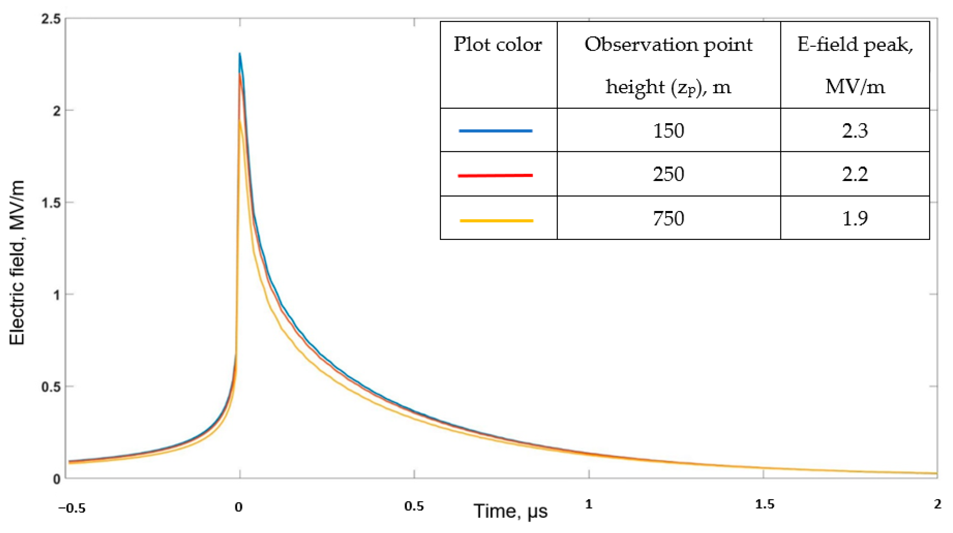In this paper, we calculate the electric fields expected to exist at the tip of a subsequent leader; they will be used for computing Coulomb’s force, which, in turn, will be compared to the friction force for warm air, as per the 3000 K friction curve shown in Figure 1. We also examine the dependence of electric field peak on the leader model input parameters, including the prospective return-stroke peak current (a proxy for the leader tip potential) and leader propagation speed, and compare model predictions with measurements.

2. Leader Model Description

The model presented by us is meant to apply to any subsequent (dart, dart-stepped, or chaotic) leader developing in a warm (reduced air density) channel, although the stepping process is not included in the model. Only the charges deposited on the leader channel (mostly in the corona sheath) are considered in computing electric fields. We assume that the leader path is straight and vertical, and we place the observation point (the point where the electric field is computed) on this path, with the leader tip approaching the point, traversing it, and moving beyond that point.

Dwyer et al. (2012, 2012) [6,7] experimentally showed that lightning leader tips are primarily responsible for X-ray emissions; thus, special attention has been paid to the electric field calculations near the leader tip. In all the electric field equations presented in this paper, $t=0$ corresponds to the time at which the leader tip passes the observation point. The leader model described below follows the ideas forming the basis of the model proposed by Cooray et al. (2009, 2010) [8,9].

We consider the leader propagating downward at a constant speed along the vertical channel that was created by the preceding return stroke, decayed, but is still warm.

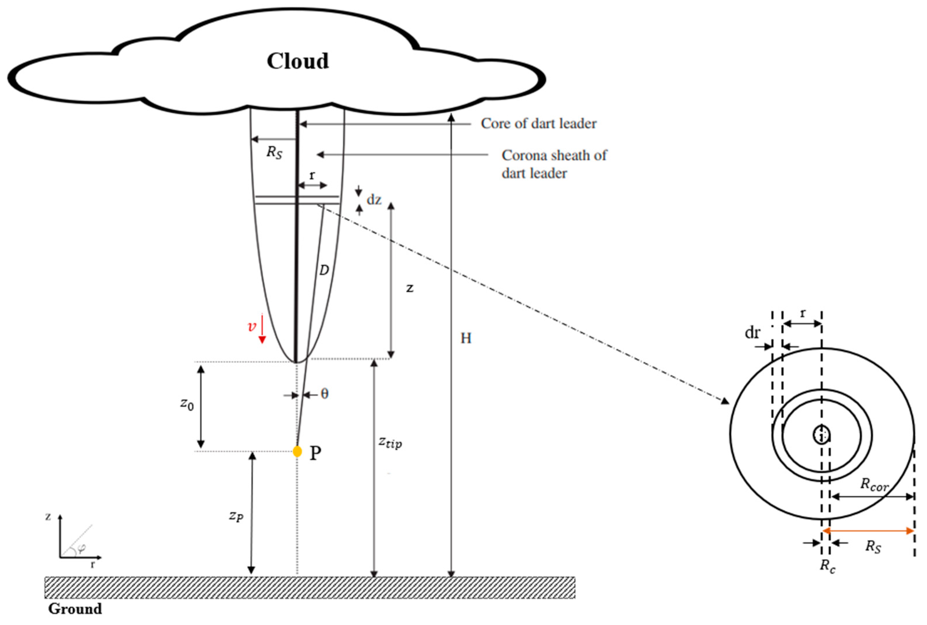
The travelling current source model used here is similar to the ones previously described by Cooray et al. (2009, 2010) [8,9], Bazelyan (1995) [10], and Thottappillil et al. (1997) [11]. It employs an approach in which the leader tip acts as downward moving current source launching a current wave moving upward, with the associated positive charge leaking radially outward to form the leader corona sheath. Each segment of the leader channel injects radial streamer current charging the corona sheath, the radius of which increases with height (see Figure 2). This is different from the distributed-source return-stroke models Maslowski et al. (2007) [12] where the distributed current sources (modeling the corona sheath charged during the leader stage) are progressively tapped by the upward-moving return-stroke front.

In Cooray et al. (2009) [8] and Cooray et al. (2010) [9], the dipole approximation was used in the field calculations and this had limited the numerical accuracy of the calculation. In the present work, the monopole approximation was used. According to this formulation, the electric field at any given point along the channel can be divided into static field produced by stationary charges, velocity field generated by moving charges and radiation field produced by accelerating charges (See Cooray et al. (2010) [13]). The results obtained show that the tip electric field is mainly determined by the static field term alone, while the contributions from the velocity and radiation fields can be neglected. For this reason, only the static field term is used in the calculations.

Furthermore, contributions from the charges inside the cloud are assumed to be insignificant in the present study. The presence of ground is also neglected.

We computed the electric field due to the leader charges at different points along its axis, both ahead and behind the leader tip. In other words, the longitudinal electric fields were computed at any point (see point P in Figure 2) along the leader axis aligned with the z-axis (directed upward with z = 0 at the ground level) of the cylindrical coordinate system. We assumed that at time $t_0$, the tip of the leader is located at height $z_{tip}$ above the ground. We introduce the equations for the static component of the electric field in Section 3.

In order to compute the electric field produced by the dart leader channel, first, we have to establish the leader channel geometry and the electric charge distribution along the channel during the leader propagation toward the ground. The maximum leader charge per unit length (${\rho }_{L0}\left(z\right)$—maximum line charge density) at height $z$ of the leader channel can be related to the prospective return-stroke current peak $I_P$. Cooray et al. (2007) [14] have shown that the maximum line charge density ${\rho }_{L0}\left(z\right)$ for $z_{tip}\ge 10 \mathrm{m}$ can be expressed based on the following empirical formula:

$${\rho }_{L0}\left(z\right)=k·\left(1-\frac{z}{H-z_{tip}}\right)·G\left(z_{tip}\right)·I_P+\frac{I_P·\left(a+b·z\right)}{1+c·z+d·z^2}·L\left(z_{tip}\right)$$

(1)

where $H$ is the cloud charge source height in $\mathbf{\left[}\mathrm{m}\mathbf{\right]}$, $z$ and $z_{tip}$ are in $\mathbf{\left[}\mathrm{m}\mathbf{\right]}$, and $I_P$ is the return-stroke peak current in $\mathbf{\left[}\mathrm{A}\mathbf{\right]}$. The other symbols represent empirical constants or functions determined in Cooray et al. (2007) [14] and given below:

$$\begin{gathered} k=5.09\times {10}^{-6} \frac{s}{m}, a=1.325\times {10}^{-8} \frac{s}{m}, b=7.06\times {10}^{-9} \frac{s}{m^2}, \\ c=2.089 \frac{1}{m}, \mathrm{and} d=1.492\times {10}^{-2} \frac{1}{m^2} \end{gathered}$$

(2)

$$G\left(z_{tip}\right)=1-\frac{z_{tip}}{H}, L\left(z_{tip}\right)=0.3·\alpha \left(z_{tip}\right)+0.7·\beta \left(z_{tip}\right)$$

(3)

$$\alpha \left(z_{tip}\right)=e^{-\frac{z_{tip}-10 m}{75 m}}, \beta \left(z_{tip}\right)=1-\frac{z_{tip}}{H}$$

(4)

Leader channel consists of a narrow hot core of radius $R_c$ and a radial corona sheath of thickness $R_{cor}$ (see inset in Figure 2) with $R_{cor}$ increasing with time. Based on Gauss’s Law, the maximum thickness of corona sheath at height $z$, $R_{cor}\left(z\right)$, can be found using the line charge density, ${\rho }_{L0}\left(z\right)$, the breakdown electric field, (assumed to be $E_c=3\times {10}^6 \mathrm{V}/\mathrm{m}$), and the electric permittivity of air, ${\epsilon }_0=8.854\times {10}^{-12} \mathrm{F}/\mathrm{m}$, as follows:

$$R_{cor}\left(z\right)=\frac{{\rho }_{L0}\left(z\right)}{2·\pi ·{\epsilon }_0·E_c}$$

(5)

Assuming that the charge at $z$ exponentially increases from 0 to ${\rho }_{L0}\left(z\right)$ with time constant $\tau =0.5 \mu \mathrm{s}$ (See Cooray et al. (2010) [9]), we express the line charge density at height $z$ seen at the observation point $\mathrm{P}$ (see Figure 2) as:

$${\rho }_L\left(z, t\prime \right)={\rho }_{L0}\left(z\right)·\left(1-e^{-t^{\prime }/\tau }\right)$$

(6)

where $t\prime$ is the retarded time required for the electric field to propagate from the source element $dz$ to the observation point $\mathrm{P}$ when the downward-moving leader tip has arrived at height $z_{tip}$. The retarded time, $t\prime$, can be computed as:

$$t\prime =\frac{z}{v}-\frac{z+z_0}{c}$$

(7)

where $v$ is the downward leader speed and $c$ is the speed of light ($c=3\times {10}^8 \mathrm{m}/\mathrm{s}$).

The total radius of the leader channel, $R_S$ (see inset in Figure 2), at height $z$ increases from $R_c$ (assumed to be equal to $1\mathrm{mm}$ according to Cooray (1996) [15]) to $R_{cor}\left(z\right)$, computed using Equation (5). Following Cooray et al. (2010) [9], we assumed that the expansion of corona sheath is exponential and the total leader channel radius is given by:

$$R_S\left(z, t\prime \right)=R_c+R_{cor}\left(z\right)·\left(1-e^{-\frac{2.3t^{\prime }}{T_s\left(z\right)} }\right)$$

(8)

where $t\prime$ is the retarded time computed using Equation (7), 2.3 is an empirical constant determined in Cooray et al. (2010) [9], and $T_S\left(z\right)$ is time during which the corona sheath attains its maximum extent at height $z$, estimated as:

$$T_s\left(z\right)=\frac{R_{cor}\left(z\right)}{v_s}$$

(9)

with $v_s$ being the speed of the streamers forming the corona sheath, which was set to $2\times {10}^5 \mathrm{m}/\mathrm{s}$, according to Cooray (2014) [16].

The volume charge density, ${\rho }_V$ in $\mathbf{\left[}\mathrm{C}/{\mathrm{m}}^3\mathbf{\right]}$, in the leader channel (including both the core and the corona sheath), assumed to be independent of the radial distance r from the leader axis, can be found as:

$${\rho }_V\left(z, t\prime \right)=\frac{{\rho }_L\left(z, t\prime \right)}{\pi ·{\left[R_S\left(z, t\prime \right)\right]}^2}$$

(10)

where $t\prime$ is the retarded time computed using Equation (7).

3. Electric Field Equations

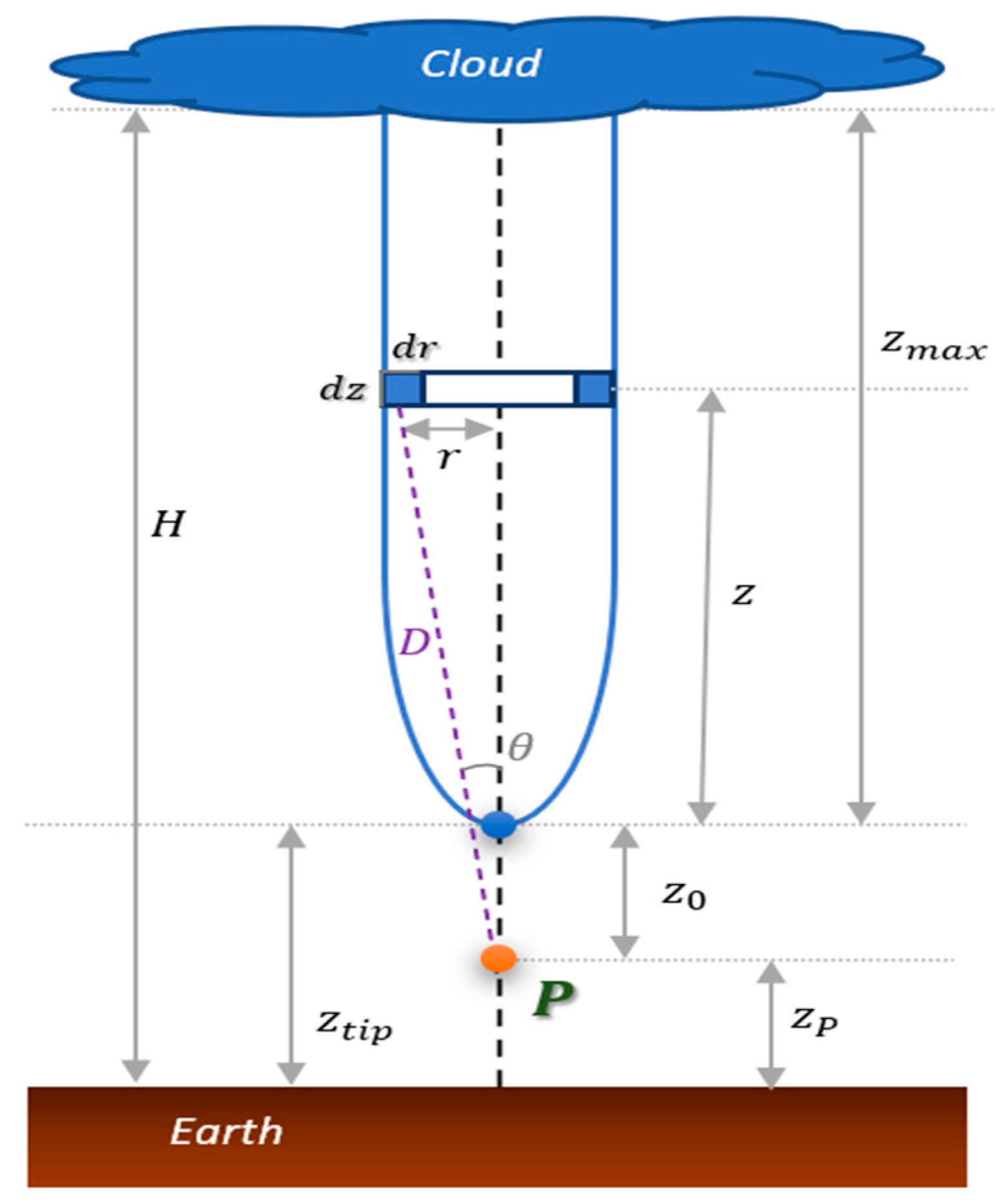
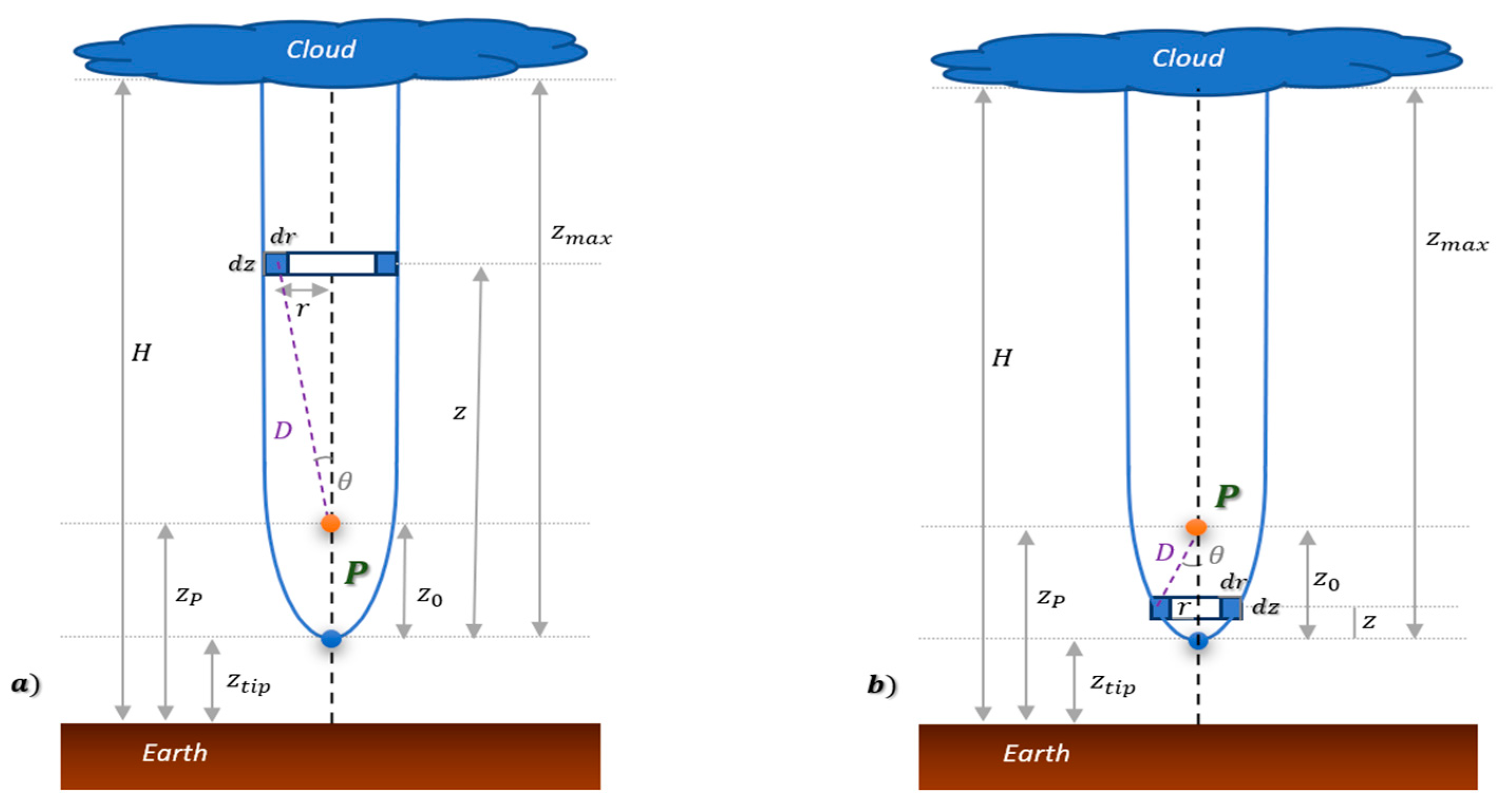
To compute the electric field produced by the leader channel, we must account for two different situations: (1) when the observation point P is in front of (below) the leader tip (between ground and the leader tip, see Figure 3) and (2) when the observation point P is behind (above) the leader tip (between the leader tip and the cloud, see Figure 4). In both cases, it is assumed that the observation point P is on the vertical axis of the lightning leader channel (see Figure 2). Therefore, the electric field produced at observation point P will only have a component along the z-axis.

Due to cylindrical symmetry of the problem, it is convenient to consider an elementary ring with radius r and square cross-sectional area $ds=dr·dz$, so that the ring volume is $dV=2\pi r·ds$, placed at height z above the leader tip (see Figure 2). For this ring, the static electric field at observation point P will be:

$$d{E}_z=\frac{{\rho }_V\left(z, t\prime \right)}{4·\pi ·{\epsilon }_0·D^2}·\cos \left(\theta \right)dV$$

(11)

where $D$ is the inclined distance between each of the points on the ring and the observation point $\mathrm{P}$ (a function of $r$, $z$, and $z_0$, see Figure 2$)$; $\theta$ is the angle shown in Figure 2 dependent on $r$, $z$, $z_0$ and $D$; $dV=2·\pi ·r·dr·dz$ is the volume of the elementary ring, and $t\prime$ is given by (7).

Thus, (11) can be written as:

$$d{E}_z=\frac{2·\pi ·r·{\rho }_V\left(z, t\prime \right)}{4·\pi ·{\epsilon }_0·D^2}·\cos \left(\theta \right)·dr·dz=\frac{{\rho }_V\left(z, t\prime \right)·r}{2·{\epsilon }_0·D^2}·\cos \left(\theta \right)·dr·dz$$

(12)

The total static electric field at observation point $\mathrm{P}$ is found by integrating $d{E}_z$ over r and z, with integration over azimuth being already accounted for by using the ring geometry.

3.1. Case 1: Point P Is in Front of the Leader Tip

In this case, the leader tip has not yet reached the observation point $\mathrm{P}$. The entire leader channel is above the observation point (see Figure 3), which allows us to treat the problem using a single equation, with $D$, $\cos \left(\theta \right)$, and the retarded time $t\prime$ given by:

$$D=\sqrt{r^2+{\left(z+z_0\right)}^2},\cos \left(\theta \right)=\frac{\left(z+z_0\right)}{D}=\frac{\left(z+z_0\right)}{\sqrt{r^2+{\left(z+z_0\right)}^2}}\mathrm{and} t\prime =\frac{z}{v}-\frac{z+z_0}{c}$$

(13)

The total static electric field produced by the entire leader channel at observation point $P$ is found using the following double integral equation:

$$E_z=\underset{0}{\overset{z_{\max }}{{\displaystyle \int }}}\left(\frac{{\rho }_V\left(z, t\prime \right)}{2·{\epsilon }_0}·\underset{0}{\overset{R_S\left(z,t^{\prime }\right)}{{\displaystyle \int }}}\left[\frac{r·\left(z+z_0\right)}{{\left(r^2+{\left(z+z_0\right)}^2\right)}^{3/2}}\right]dr\right)dz$$

(14)

where $z_{\max }$ is the maximum value of $z$, which is the difference between $H$ and $z_{tip}$.

Evaluating the integral over r from 0 to $R_S\left(z,t\prime \right)$, for given $z$ and $z_0$, we obtained:

$$E_z=\underset{0}{\overset{z_{\max }}{{\displaystyle \int }}}\left(\frac{{\rho }_V\left(z, t\prime \right)}{2·{\epsilon }_0}·\left[1-\frac{\left(z+z_0\right)}{{\left(R_S^2\left(z,t\prime \right)+{\left(z+z_0\right)}^2\right)}^{\frac{1}{2}}}\right]\right)dz$$

(15)

3.2. Case 2: Point P Is behind the Leader Tip

In this case, the leader tip has passed the observation point P, so that part of the leader channel is above the observation point (see Figure 4a) and part of the channel is below the observation point (see Figure 4b).

The electric field component produced by the leader charges above the observation point $\mathrm{P}$ can be computed in a way similar to that presented in Section 3.1 for Case 1. The leader charges below the observation point will produce an electric field component with opposite direction, so that the total electric field produced by the entire leader channel at observation point $\mathrm{P}$ can be expressed as:

$$E_z=E_{z1}-E_{z2}$$

(16)

where $E_{z1}$ is the electric field due to the leader charges at or above the observation point and $E_{z2}$ is the electric field due to the charges below the observation point.

For the leader channel at or above the observation point $\mathrm{P}$, ($z\ge z_0$) we can write (see Figure 4a):

$$D=\sqrt{r^2+{\left(z-z_0\right)}^2},\cos \left(\theta \right)=\frac{\left(z-z_0\right)}{D}=\frac{\left(z-z_0\right)}{\sqrt{r^2+{\left(z-z_0\right)}^2}}\mathrm{and} t\prime =\frac{z}{v}-\frac{z-z_0}{c}$$

(17)

Thus, $E_{z1}$ will be:

$$E_{z1}=\underset{z_0}{\overset{z_{\max }}{{\displaystyle \int }}}\left(\frac{{\rho }_V\left(z,t\prime \right)}{2·{\epsilon }_0}·\left[1-\frac{\left(z-z_0\right)}{{\left(R_S^2\left(z,t\prime \right)+{\left(z-z_0\right)}^2\right)}^{\frac{1}{2}}}\right]\right)dz$$

(18)

For the leader channel below the observation point $\mathrm{P}$ ($z<z_0$), we have (see Figure 4b):

$$D=\sqrt{r^2+{\left(z_0-z\right)}^2},\cos \left(\theta \right)=\frac{\left(z_0-z\right)}{D}=\frac{\left(z_0-z\right)}{\sqrt{r^2+{\left(z_0-z\right)}^2}}\mathrm{and} t\prime =\frac{z}{v}-\frac{z_0-z}{c}$$

(19)

As a result, $E_{z2}$ is given by:

$$E_{z2}=\underset{0}{\overset{z_0}{{\displaystyle \int }}}\left(\frac{{\rho }_V\left(z,t\prime \right)}{2·{\epsilon }_0}·\left[1-\frac{\left(z_0-z\right)}{{\left(R_S^2\left(z,t\prime \right)+{\left(z_0-z\right)}^2\right)}^{\frac{1}{2}}}\right]\right)dz$$

(20)

The total electrostatic field for Case 2 is obtained by algebraically adding the contributions given by (18) and (20), as per Equation (16).

4. Analysis and Results

4.1. Typical Subsequent-Leader Electric Field Waveform

We first use the model described in Section 3 for computing the electric field waveform at an observation point P located 250 m above ground level for a typical subsequent leader with the following parameters: $I_p=12 \mathrm{kA}, v=1\times {10}^7 \mathrm{m}/\mathrm{s}, H=5 \mathrm{km}$. Our model prediction is shown in Figure 5.

Note that the electric field in Figure 5 rapidly rises as the leader tip approaches the observation point, peaks when the leader tip passes through the observation point, and then begins to decline once the observation point is inside the leader channel. The electric field peak is about 2.3 MV/m and the half-peak width is 0.14 µs.

Modeling results presented in this subsection confirm that the electric field peak produced by a subsequent leader can briefly reach some megavolts per meter, which may be sufficient to cause runaway electron avalanches in warm (reduced air density) channel left behind by the preceding return stroke. In Section 4.2 below, we will perform a sensitivity analysis and show that the electric field peak associated with a subsequent leader can be as high as 20 MV/m, certainly enough to overcome the friction force (see the red curve in Figure 1) and to produce energetic radiation in a warm channel.

4.2. Sensitivity Analysis

We now examine how variations in the input parameters affect the model-predicted electric field waveforms. The following model input parameters will be considered: observation point height, return-stroke peak current, leader channel length, and leader speed. Model formulation described in Section 2 and Section 3 is used throughout this section. Results of the sensitivity analysis are shown in Figure 6, Figure 7, Figure 8 and Figure 9. In each Figure, we vary one of the input parameters, while keeping the other three at their nominal values (those used in Section 4.1).

In Figure 6, one can see how the electric field peak increases with decreasing the height of observation point above ground ($z_p$). Both the highest peak and the largest half-peak-width correspond to $z_p$ = 150 m. Note that the influence of this parameter is relatively small. The E-field peak does not exceed the value (~4 MV/m) required for ambient electrons to run away in warm channels that are traversed by subsequent lightning leaders.

In Figure 7, we see that as the peak current increases from 12 kA to 55 kA the electric field peak increases from 2.2 MV/m to 10 MV/m. Thus, there appears to be a linear relationship between the prospective return-stroke peak current, which can be viewed as a proxy for leader tip potential, and the electric field peak. For higher peak currents (25 kA and 55 kA), the E-field peak exceeds the value (~4 MV/m) required for ambient electrons to run away in warm channels that are traversed by subsequent lightning leaders.

The maximum leader channel length does not significantly influence the electric field (see Figure 8), as expected, since the largest contributions to the electric field come from the charges located near within 200 m or so of the leader tip. The E-field peak does not exceed the value (~4 MV/m) required for ambient electrons to run away in warm channels that are traversed by subsequent lightning leaders.

In Figure 9, one can see that the leader with a $0.5\times {10}^7 \mathrm{m}/\mathrm{s}$ speed has the highest electric field peak and largest half-peak width, and the leader with $1.5\times {10}^7 \mathrm{m}/\mathrm{s}$ speed has the lowest electric field peak and smallest half-peak width. There appears to be an inverse relationship between the leader speed and the electric field peak, with slower leaders producing higher electric fields. For the slowest leader ($0.5\times {10}^7$ m/s), the E-field peak exceeds the value (~4 MV/m) required for ambient electrons to run away in warm channels that are traversed by subsequent lightning leaders.

5. Discussion and Implications for X-ray/Gamma-ray Production by Subsequent-Stroke Leaders

As noted in the Introduction, subsequent leaders discussed in this paper traverse warm (reduced air density) channels. For such channels, the critical runaway breakdown field is considerably (about an order of magnitude) lower than in cold air. 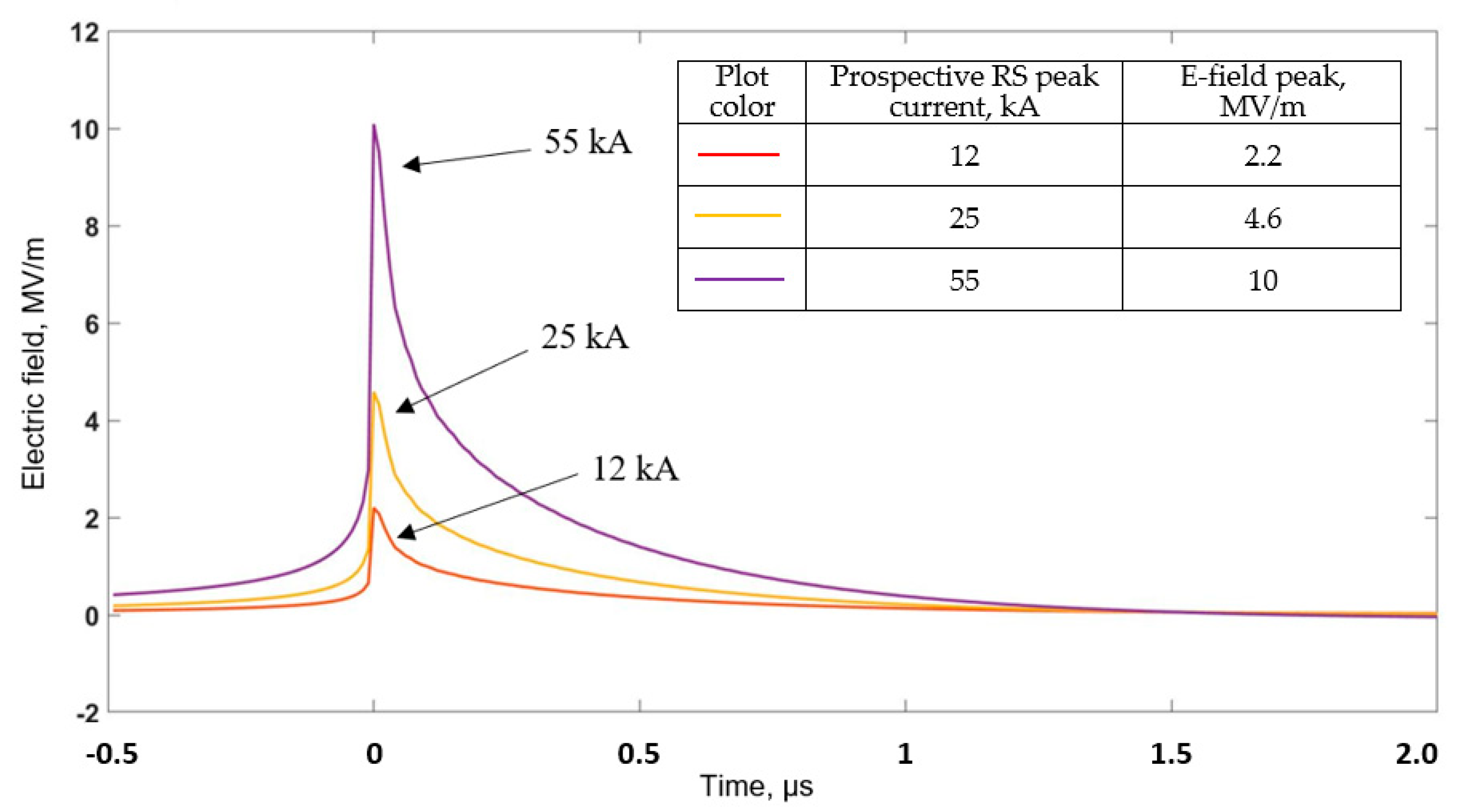We calculated the electric fields expected to exist at the tip of a subsequent leader, which were used for computing the Coulomb force, which, in turn, was compared to the friction force for warm air, as per the 3000 K friction curve shown in Figure 1. We also examined the dependence of electric field peak on the leader model input parameters, including the prospective return-stroke peak current (a proxy for the leader tip potential) and leader propagation speed.

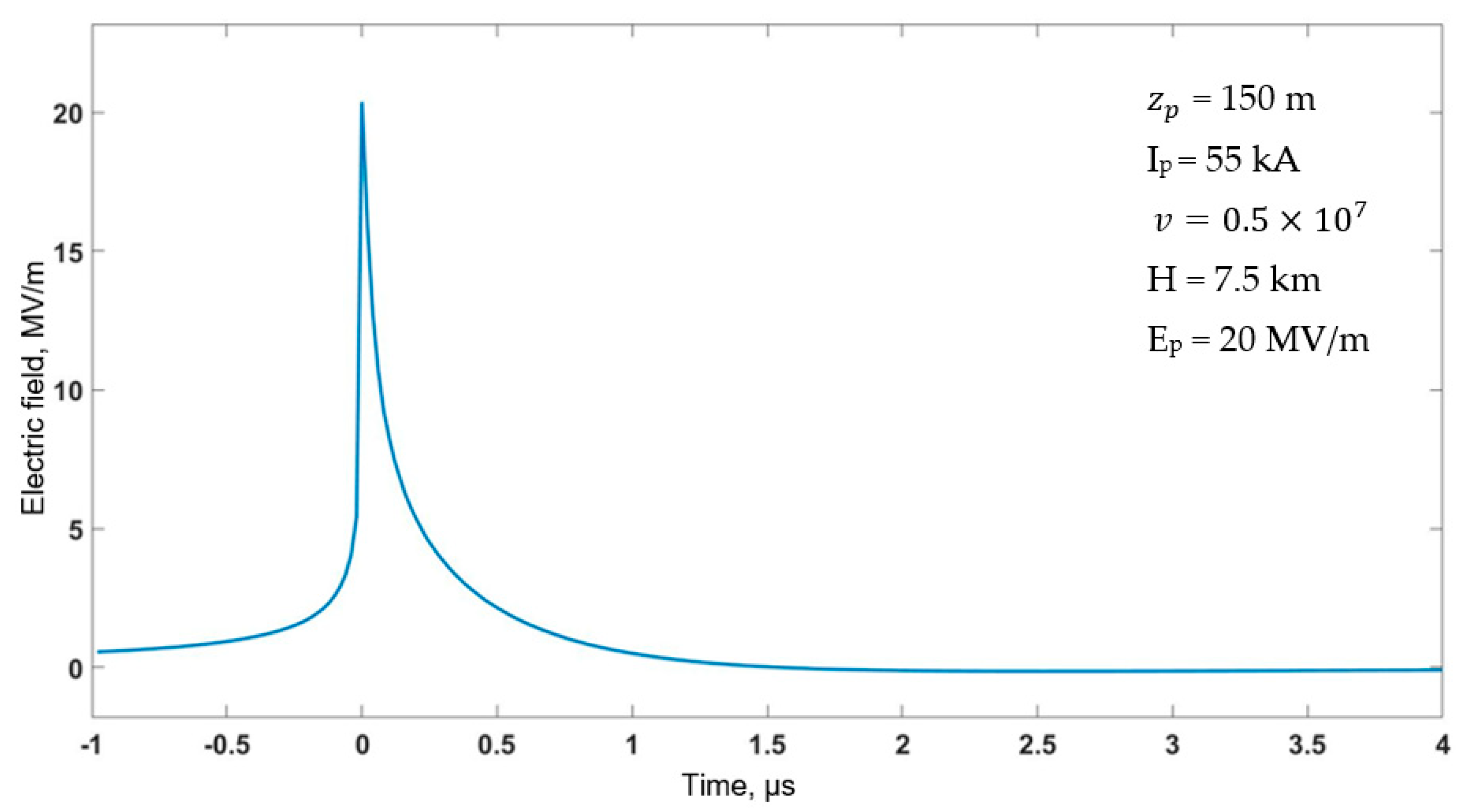
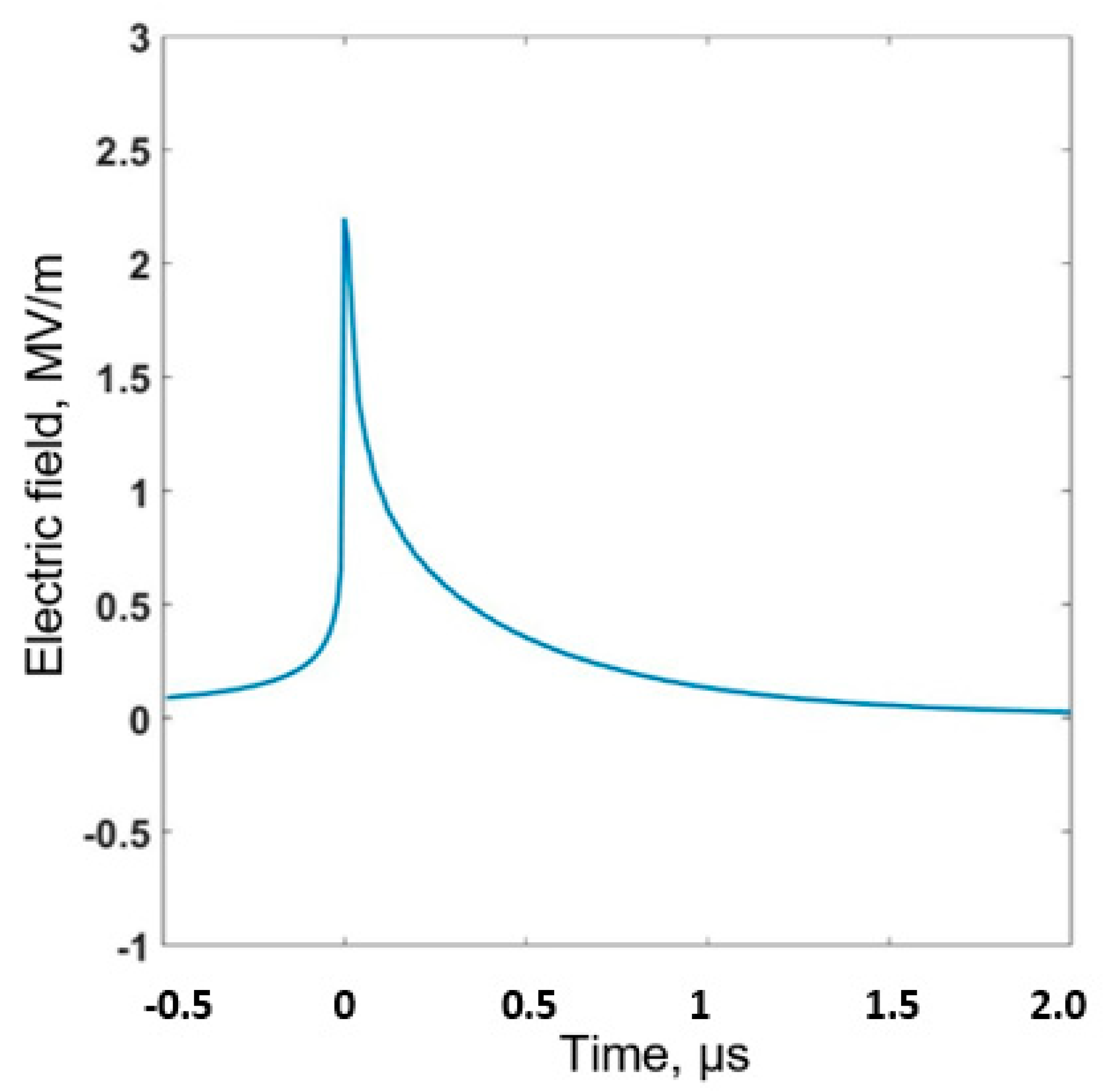
Based on the sensitivity analysis presented in Section 4.2 above, we found the “worst case” combination of model input parameters, such that the electric field peak is maximized: $z_p=$150 m, $I_p=$55 kA, H = 7.5 km, and $v=0.5\times {10}^7 \mathrm{m}/\mathrm{s}.$ For these values, the electric field peak predicted by our model is 20 MV/m (see Figure 10). The Coulomb force acting on an electron corresponding to a field of 20 MV/m is considerably larger than the peak of the friction curve for warm air (~4 MV/m; see red curve in Figure 1) allowing all electrons (regardless of their energy) to run away. This means that a relativistic runaway process does not require the presence of a super-energetic cosmic-ray particle and can start from the ambient electron distribution. The event presented in Figure 10 can be viewed as representing the very intense X-ray/gamma-ray producer reported by Mallick et al. (2012) ([2], Figure 7, bottom panel). That stroke followed the previously formed (warm) channel to ground and had the NLDN-reported peak current of 55 kA and the leader speed, inferred from the measured leader duration and assumed total channel length of 7.5 km, of $8.3\times {10}^6 \mathrm{m}/\mathrm{s}$, values similar to those used in computing the E-field waveform shown in Figure 10.

The present study provides additional support to the elevated-temperature scenario (previously considered by Mallick et al. (2012) [2] and Tran et al. (2015, 2019) [3,17]), which requires realistic (confirmed by modeling) electric fields and no energetic electrons from external sources. Furthermore, we have shown that subsequent-leader electric fields can be high enough to overcome the warm-air friction curve, but not strong enough to overcome the cold-air friction curve, the latter one being applicable to first-stroke leaders. This implies that in, say, a two-stroke flash with both strokes having the same intensity, the second stroke may be producing X-rays/gamma-rays, while the first stroke may not.

6. Summary and Concluding Remarks

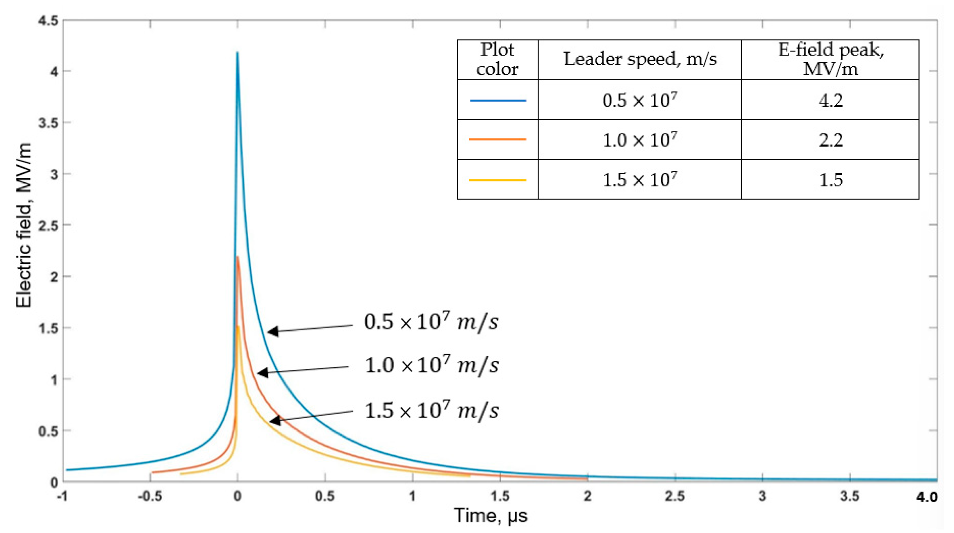
A new formulation of the model for computing E-fields both ahead and behind of the downward moving leader tip was developed. The electric field waveform on the axis of vertically descending leader is a sharp pulse with its peak corresponding to the leader tip passing through the observation point.

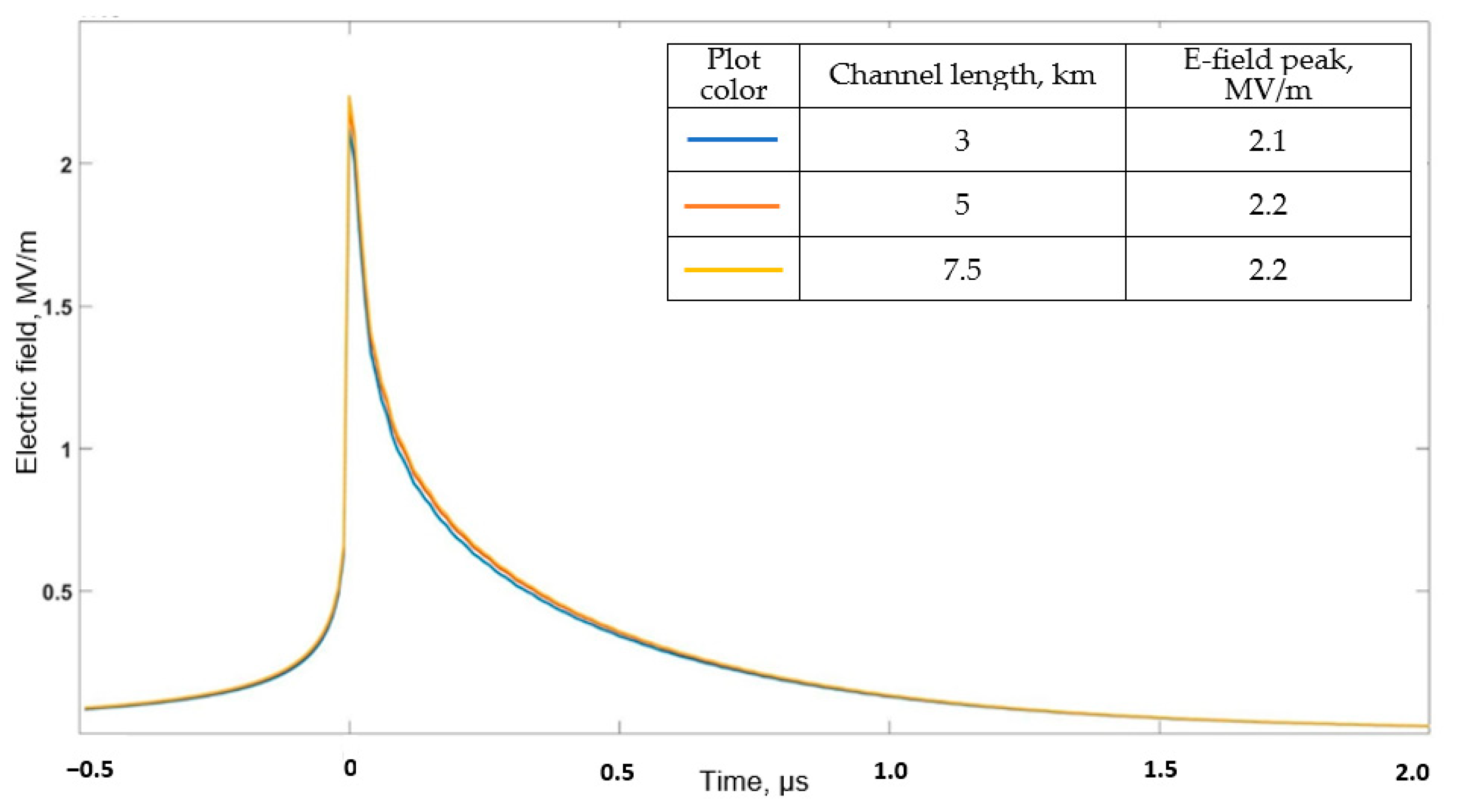
Dependence of the E-field peak on model input parameters was examined. The E-field peak increases with increasing the prospective return-stroke peak current (a proxy for leader tip potential) and with decreasing the leader speed. This is an interesting finding, as generally, higher peak-current strokes tend to have faster leaders; thus, high peak-current strokes with slow leaders may be uncommon, but they are expected to be prolific X-ray/gamma-ray producers.

For a free electron to run away, the Coulomb force acting on that electron must be greater than the friction force (rate of electron energy loss per unit distance), the latter being a function of electron energy. In this study, we computed subsequent-leader electric fields to see if their associated Coulomb forces can overcome the warm-air friction force acting on ambient electrons with energies less than 30 eV or so. We found that for realistic model input parameters, the E-field peak can exceed the value (~4 MV/m) required for ambient electrons to run away in warm channels that are traversed by subsequent lightning leaders.

Mallick et al. (2012) [2] discovered that subsequent strokes can be more prolific X-ray/gamma-ray producers than first strokes in the same flash. They hypothesized that their unexpected observation could be explained by the fact that subsequent leaders traversed still warm (3000 K) remnants of previously created but decayed channels, for which the friction curve is considerably lower than for cold air. In this paper, we confirmed Mallick et al.’s hypothesis by showing that subsequent-leader electric fields can be high enough to overcome the warm-air friction curve, but not enough to overcome the cold-air friction curve, the latter one being applicable to first-stroke leaders.

References

1. Dwyer, J.R. Implications of X-ray emission from lightning. Geophys. Res. Lett. 2004, 31, L12102. [Google Scholar] [CrossRef]
2. Mallick, S.; Rakov, V.A.; Dwyer, J.R. A study of X-ray emissions from thunderstorms with emphasis on subsequent strokes in natural lightning. J. Geophys. Res. 2012, 117, D16107. [Google Scholar] [CrossRef] [Green Version]
3. Tran, M.D.; Kereszy, I.; Rakov, V.A.; Dwyer, J.R. On the Role of Reduced Air Density Along the Lightning Leader Path to Ground in Increasing X-Ray Production Relative to Normal Atmospheric Conditions. Geophys. Res. Lett. 2019, 46, 9252–9260. [Google Scholar] [CrossRef]
4. Rakov, V.A.; Uman, M.A. Lightning: Physics and Effects; Cambridge University Press: New York, NY, USA, 2003. [Google Scholar]
5. Uman, M.A.; Voshall, R.E. Time interval between lightning strokes and the initiation of dart leaders. J. Geophys. Res. 1968, 73, 497–506. [Google Scholar] [CrossRef]
6. Dwyer, J.R.; Schaal, M.M.; Cramer, E.; Arabshahi, S.; Liu, N.; Rassoul, H.K.; Hill, J.D.; Jordan, D.M.; Uman, M.A. Observation of a Gamma-Ray Flash at Ground Level in Association with a Cloud-to-Ground Lightning Return Stroke. J. Geophys. Res. 2012, 117, A10303. [Google Scholar] [CrossRef] [Green Version]
7. Dwyer, J.R.; Smith, D.M.; Cummer, S.A. High-energy atmospheric physics: Terrestrial gamma-ray flashes and related phenomena. Space Sci. Rev. 2012, 173, 133–196. [Google Scholar] [CrossRef] [Green Version]
8. Cooray, V.; Becerra, M.; Rakov, V.A. On the electric field at the tip of dart leaders in lightning flashes. J. Atmos. Sol.-Terr. Phys. 2009, 71, 1397–1404. [Google Scholar] [CrossRef]
9. Cooray, V.; Dwyer, J.R.; Rakov, V.A.; Rahman, M. On the mechanism of X-ray production by dart leaders of lightning flashes. J. Atmos. Sol.-Terr. Phys. 2010, 72, 848–855. [Google Scholar] [CrossRef]
10. Bazelyan, E.M. Waves of Ionization in Lightning Discharge. Plasma Pysics Rep. 1995, 21, 497–506. [Google Scholar]
11. Thottappillil, R.; Rakov, V.A.; Uman, M.A. Distribution of Charge along the Lightning Channel: Relation to Remote Electric and Magnetic Fields and to Return-Stroke Models. J. Geophys. Res. 1997, 102, 6987–7006. [Google Scholar] [CrossRef]
12. Maslowski, G.; Rakov, V.A. Equivalency of Lightning Return-Stroke Models Employing Lumped and Distributed Current Sources. IEEE Trans. Electromagn. Compat. 2007, 49, 123–132. [Google Scholar] [CrossRef]
13. Cooray, V.; Cooray, G. The electromagnetic fields of an accelerating charge: Applications in lightning return stroke models. IEEE Trans. Electromagn. Compat. 2010, 52, 944–955. [Google Scholar] [CrossRef]
14. Cooray, V.; Rakov, V.A.; Theethayi, N. The Lightning Striking Distance—Revisited. J. Electrost. 2007, 65, 296–306. [Google Scholar] [CrossRef]
15. Cooray, V. A Model for dart Leaders in Lightning Flashes. J. Atmos. Electr. 1996, 16, 145–159. [Google Scholar]
16. Cooray, V. The Lightning Flash, 2nd ed.; IET: London, UK, 2014. [Google Scholar]
17. Tran, M.D.; Rakov, V.A.; Mallick, S.; Dwyer, J.R.; Nag, A.; Heckman, S. A terrestrial gamma-ray flash recorded at the Lightning Observatory in Gainesville, Florida. J. Atmos. Sol.-Terr. Phys. 2015, 136, 86–93. [Google Scholar] [CrossRef] [Green Version]
Figure 1. The dynamic friction curves showing the friction force (rate of energy loss per unit distance) experienced by an electron as a function of electron energy for cold air and for air at 3000 K. The curves include the effects of both inelastic scattering of the electron with air molecules and Bremsstrahlung emission. The horizontal lines represent the Coulomb force acting on the electron (eE, where E is the electric field intensity and e is the electron charge) corresponding to E = 1 MV/m and E = 5 MV/m (see the right vertical scale). Electrons can run away to relativistic energies when the Coulomb force is greater than the friction force. For cold air and E = 5 MV/m, only electrons with energy greater than 5 keV can run away, while for the air at 3000 K, all electrons can do so. Adapted from Dwyer (2004) [1] and Tran et al. (2019) [3].
Applsci 12 07520 g001
Figure 2. The downward-extending leader geometry used in the modeling. The leader moves along a previously created, but decayed channel, not shown in this Figure. Adapted from Cooray et al. (2010) [9].
Applsci 12 07520 g002
Figure 3. Case 1: Observation point P is in front of (below) the leader tip located at height z t i p .
Applsci 12 07520 g003
Figure 4. Case 2: Observation point P is behind (above) the leader tip located at height z t i p . (a) Ring element/charges above observation point P ; (b) Ring element/charges below observation point P .
Applsci 12 07520 g004
Figure 5. The variation of the electric field at a point located 250 m above ground as the descending leader passes through it, computed using the formulation presented in Section 3 of this paper. The field peak at t = 0 corresponds to the leader tip being at the observation point, the part of the field waveform at t < 0 corresponds to the tip being above the observation point, and the part at t > 0 corresponds to the tip being below the observation point. Full time scale is 2.5 µs.
Applsci 12 07520 g005
Figure 6. Electric field waveforms at points located 150 m, 250 m, and 750 m above ground as the leader passes through each of them. In all three cases, t = 0 corresponds to z t i p = z p . The return-stroke peak current I p = 12 kA, H = 5 km, and the leader speed v = 10 7   m / s . Full time scale is 2.5 µs.
Applsci 12 07520 g006
Figure 7. Electric field at a point located 250 m above ground as the leader passes through it, computed for prospective return-stroke (RS) peak currents of 12 kA, 25 kA, and 55 kA. Other model input parameters were as follows: H = 5 km, and v = 10 7   m / s . Full time scale is 2.5 µs.
Applsci 12 07520 g007
Figure 8. Electric field waveforms at a point located 250 m above ground as the leader passes through it, computed for maximum leader channel lengths of 3 km, 5 km, and 7.5 km. The return-stroke peak current is I p = 12 kA and the leader speed is 10 7   m / s . Full time scale is 2.5 µs.
Applsci 12 07520 g008
Figure 9. Electric field waveforms at a point located 250 m above ground as the leader passes through it, computed for leader speeds of 0.5 × 10 7   m / s , 1.0 × 10 7   m / s , and 1.5 × 10 7   m / s . Other model input parameters were as follows: I p = 12 kA and H = 5 km. Full time scale is 5 µs.
Applsci 12 07520 g009
Figure 10. Electric field waveform corresponding to the “worst case” combination of the model input parameters: z p = 150 m, I p = 55 kA, H = 7.5 km, and v = 0.5 × 10 7   m / s . Full time scale is 5 µs.
Applsci 12 07520 g010