Abstract
In the edge computing and network communication environment, important image data need to be transmitted and stored securely. Under the condition of limited computing resources, it is particularly necessary to design effective and fast image encryption algorithms. One-dimensional (1D) chaotic maps provide an effective solution for real-time image encryption, but most 1D chaotic maps have only one parameter and a narrow chaotic interval, which has the disadvantage of security. In this paper, a new compound 1D chaotic map composed of a logistic map and tent map is proposed. The new system has two system parameters and an arbitrarily large chaotic parameter interval, and its chaotic signal is evenly distributed in the whole value space so it can improve the security in the application of information encryption. Furthermore, based on the new chaotic system, a fast image encryption algorithm is proposed. The algorithm takes the image row (column) as the cyclic encryption unit, and the time overhead is greatly reduced compared with the algorithm taking the pixel as the encryption unit. In addition, the mechanism of intermediate key associated with image content is introduced to improve the ability of the algorithm to resist chosen-plaintext attack and differential attack. Experiments show that the proposed image encryption algorithm has obvious speed advantages and good cryptographic performance, showing its excellent application potential in secure network communication.
1. Introduction
In today’s networking information age, human communication and information exchange mainly rely on network digital communication, and multimedia digital communication plays an important role in human digital communication. Therefore, the amount of multimedia data to be stored and transmitted is increasing. The protection of data security and privacy has become an urgent problem to be solved. Unfortunately, traditional encryption schemes such as AES, DES and RSA are mainly designed for text data so they are not suitable for image security applications [1,2], especially for real-time encryption of big data. Because of the huge amount of image data, high information redundancy and strong correlation urges researchers to seek efficient image encryption algorithms. Therefore, some new image encryption schemes based on different theories and technologies have attracted the attention of researchers. Among them, chaos-based cryptography shows obvious advantages in the field of image encryption [3,4,5,6,7].
Since the sequence of state values generated by the chaotic system have aperiodic ergodicity and extreme sensitivity to initial conditions, chaotic sequence is a pseudo-random sequence with unpredictability. These characteristics of chaotic sequences coincide with the basic requirements of cryptography. As a result, chaotic sequence has a good value in cryptography, and the image encryption technology based on chaos has attracted more and more attention [5,7,8,9]. Generally speaking, chaotic systems are divided into high-dimensional continuous time systems described by differential equations and low-dimensional discrete time systems described by iterative maps. The structure of a low-dimensional discrete chaotic map is simple, the software calculation speed is fast, and the hardware implementation is easier. However, some common low-dimensional discrete chaotic maps have the following defects: the number of parameters is small, and the map is easy to predict. Moreover, the range of parameters with chaotic behavior are narrow and the distribution of state values is not uniform. For example, there are such systems as the famous logistic map [10], tent map [11], sine map [12], etc. Due to the above shortcomings of such chaotic systems, information encryption brings the risk of security reduction. On the contrary, the high-dimensional continuous time chaotic system has more variables and parameters, and the parameter interval of chaotic behavior is large. However, this kind of complex dynamical system described by differential equations is more difficult to implement by hardware and requires more time overhead for software calculation, so it is not suitable for real-time encryption applications.
Constructing new chaotic systems with a simple structure and high unpredictability has become an important issue for many cryptologists and researchers [13,14,15,16,17]. Ramasamy et al. [18] proposed an enhanced logistic map (ELM) and applied it in an image encryption scheme based on block scrambling and modified zigzag transformation. The authors claim that the method is secure and computationally efficient based on the analysis of the proposed method. Gupta et al. [19] proposed a lightweight image encryption algorithm based on a logistic-tent map and crossover operator. The extensive experiments of performance and security assessment show that the proposed image encryption scheme is secure enough to withstand all potential cryptanalytic attacks. Tong et al. [20] proposed a new perturbed high-dimensional chaotic map and applied it to design a new encryption scheme. Although the encryption scheme can obtain satisfactory security, its encryption speed cannot meet the requirements of real-time encryption. Pak et al. [21] proposed a new 1D chaotic system and applied it to color image encryption. Although the encryption system has acceptable speed, it has security defects. Some researchers have analyzed the encryption system [22,23]. Hua et al. [24] proposed a new two-dimensional (2D) chaotic system called a 2D-LASM and applied it to design an image encryption scheme. Although the authors claim that the system has a high security level, Feng et al. [25] did a detailed cryptanalysis for it and cracked the cryptosystem. Wang et al. [26] proposed a fast image encryption algorithm based on a logistic map, which has high encryption speed. However, the logistic map is not secure enough because of its small chaotic space and is vulnerable to brute force attacks. Although some existing image encryption algorithms have high security [6,27,28,29,30,31,32], many of them are only suitable for specific types of image encryption, such as color image and medical image, and cannot handle all types of digital images. The defects of these existing image encryption schemes have aroused our motivation to design a new image encryption scheme that is safe, fast and universal.
In this paper, a new discrete chaotic map composed of a logistic map and tent map is proposed. The compound map has a very wide range of chaotic parameters and the system structure is simple, which can realize fast calculation and is more suitable for real-time image encryption processing. It can also generate a uniformly distributed sequence filled with the whole state value space, which validates its application in cryptography with a large enough secret key space and can resist the violent attack of key exhaustion. The uniformly distributed state values can better resist the attack of statistical analysis. Through a series of famous chaos theory tools, such as theoretical proof of state boundedness, Lyapunov exponent, bifurcation diagram, approximate entropy, time-series diagram and cobweb graph, we prove the highly chaotic behavior of the proposed compound chaotic map. Based on the new chaotic map system, we also designed a new high-speed image encryption scheme. In this new image encryption scheme, we adopt an improved permutation-substitution strategy which completes the permutation of image pixel positions and the substitution of pixel values simultaneously and takes the image row or column as the cyclic processing unit instead of a single pixel as the cyclic processing unit, which greatly improves the security and speed of the scheme. In addition, the new image encryption scheme can achieve satisfactory encryption effects with a small number of encryption rounds. The number of encryption rounds can be adjusted according to the actual requirement. We use histogram analysis, information entropy, key analysis, and ciphertext sensitivity to plaintext and key to evaluate the efficiency and security of the scheme. In the same experimental environment, we also compare this scheme with some latest encryption schemes. The comparison results show that the new scheme is superior to other schemes in safety and speed. The main contributions of this work are as follows:
(1) A new model of one-dimensional discrete compound chaotic map is proposed, which has two system parameters and unlimited parameter range. The parameter interval of this system, which can generate chaotic phenomena, is much wider than the existing 1D maps, and the generated chaotic signals are more evenly distributed in the range of (0, 1). Therefore, the system used for information encryption can obtain larger key space and better security.
(2) Based on the new chaotic system, a new image encryption algorithm is proposed, which combines the traditional permutation and substitution operations and simultaneously realizes the pixel position permutation and pixel value substitution. It can not only improve the encryption speed, but also increase the difficulty of deciphering the key. In addition, the encryption operation cycle process takes rows (columns) as processing units instead of pixels as processing units, which can significantly improve the encryption speed.
(3) The intermediate key is related to the content of the image to be encrypted. By introducing this mechanism, the ability of the cryptosystem to resist chosen-plaintext attack is improved. In addition, the sensitivity of ciphertext to plaintext is also enhanced, which leads to the improvement of the performance of the algorithm against differential cryptanalysis.
The rest of this paper is arranged as follows: Section 2 introduces the proposed new chaotic map system and proves its strong chaotic behavior with common chaos theory tools. Section 3 introduces the proposed new image encryption scheme based on this chaotic map. Section 4 tests the performance and security analysis of the proposed new image encryption scheme. The last section is the summary of the whole paper.
2. The Proposed New One-Dimensional Chaotic Map
In this paper, a new one-dimensional compound chaotic system is constructed based on the 1D logistic map and 1D tent map. First, we briefly introduce the mathematical models of the logistic map and tent map and their basic characteristics (Lyapunov exponent and bifurcation diagram).
2.1. Logistic Map (LM)
The mathematical model of the logistic map (LM) system is shown in Equation (1) [10].
In Equation (1), xn represents the state values of the system at the n-th discrete time point (n = 0, 1, …), x0 represents the initial state value of the system. b is the control parameter of the system. When , the function is a map: , and the iterative sequence {x0, x1, x2, …} generated by the initial state value of is aperiodic (or the period is infinite and the state value is not repeated) and is seemingly an irregular (random) sequence. However, the state values in the sequence are bounded (that is, the value of , will not run out of the range of (0, 1), which is called the attractor). Figure 1a is a graph of the Lyapunov exponent of the logistic map changing with parameter b. Among them, the formula for calculating the Lyapunov exponent LE of 1D maps is shown in formula (2).
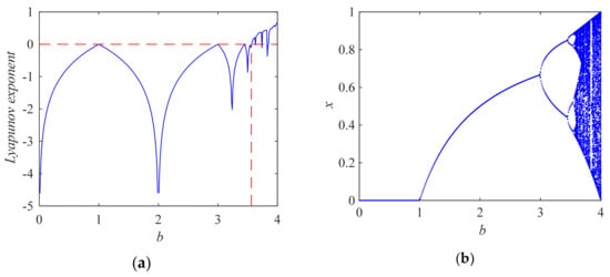
Figure 1.
Lyapunov exponent and bifurcation diagram of logistic map. (a) The graph of Lyapunov exponent versus parameter b; (b) bifurcation diagram of system state quantity versus parameter b.
In formula (2), is the value of the derivative function of the mapping function at xn. In actual calculation if the value of N is large enough, the Lyapunov exponent will converge to a fixed constant. As long as it is found that the Lyapunov exponent starts to stabilize (no longer changes with the increase of N), then N can be regarded as satisfying the condition of . A positive Lyapunov exponent means chaos. Figure 1 shows the variation of the Lyapunov exponent and bifurcation diagram of the system with parameter b. As can be seen from Figure 1a, when the parameter b satisfies , the system goes into a chaotic state. When b = 4, the maximum Lyapunov exponent occurs, which is LEmax = 0.6931. Figure 1b is the bifurcation diagram of Logistic map changing with parameter b, which is consistent with the phenomenon revealed in Figure 1a; that is, when the parameter b satisfies , the value number of the system state is infinite, and with the increase of b, the value of the system state gradually fills the whole range of (0, 1).
2.2. Tent Map (TM)
The mathematical model of the tent map (TM) [11] system is shown in Equation (3):
In Equation (3), xn represents the state values of the system at the n-th discrete time point (n = 0, 1, 2, …). x0 represents the initial state value of the system, and b is the control parameter of the system. Figure 2 shows the variation of the Lyapunov exponent and bifurcation diagram of the tent map with parameter b. Figure 2a is the Lyapunov exponent curve of the tent map with a system parameter b. When b = 4, the maximum Lyapunov exponent occurs, which is LEmax = 0.6931. Figure 2b is the state value bifurcation diagram of the tent map with system parameter b. As can be seen from Figure 2, when , system (3) enters the chaotic state.
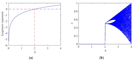
Figure 2.
Lyapunov exponent and bifurcation diagram of tent map. (a) The graph of Lyapunov exponent versus parameter b; (b) bifurcation diagram of system state quantity versus parameter b.
The disadvantages of the above two systems are as follows: First, the parameter interval of the system where chaos occurs is relatively narrow (the chaotic parameter interval of LM system is , and the chaotic parameter interval of TM system is ). Second, when b < 4, the value of the system state cannot fill the whole space range of (0, 1).
2.3. Logistic-Tent Map (LTM)
In this paper, a compound chaotic system, named the logistic-tent map (LTM) system, is proposed. The mathematical model of LTM system is shown in formula (4)
where is the state variable of the system, a and b are two control parameters of the system, and .
2.3.1. Boundedness of State Value Distribution of LTM System
Properties 1.
When ,, system (4) is a mapping: .
Proof.
The monotonicity of the function in the interval can be proven according to the positive and negative of the function derivative. The derivative function of is
It can be concluded from Equation (5) that
when , owing to > 0, so the function f(xn) increases monotonically over the interval (0, 0.5). It can be seen from this that f(0) < f(xn) < f(0.5), namely: 0 < f(xn) < 1.
When , owing to <0, the function f(xn) decreases monotonically over the interval (0.5, 1). It can be seen from this that f(1) < f(xn) < f(0.5), namely: 0 < f(xn) < 1.
Therefore, if , then 0 < f(xn) < 1. The proof is complete. □
Property 1 shows that the state values of LTM are bounded and conform to the attractor condition.
2.3.2. Lyapunov Exponent and Bifurcation Diagram of LTM System
The Lyapunov exponent of system (4) is positive in all ranges of the parameter interval of b (see Figure 3a, where a = 6). When b = 0.35, the Lyapunov exponent has the maximum value of LEmax = 0.6934. The bifurcation diagram (see Figure 3b, where a = 6) of state values of the system also proves that the system is aperiodic in the whole parameter value range (unlimited values/no repetition), and the state values can evenly fill the whole value space in (0, 1). These characteristics of the LTM system will bring better security for information encryption.
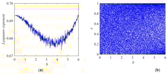
Figure 3.
Lyapunov exponent and bifurcation diagram of LTM. (a) The graph of Lyapunov exponent versus parameter b; (b) bifurcation diagram of system state quantity versus parameter b.
2.3.3. Approximate Entropy of LTM System
Approximate entropy can measure the randomness and complexity of the time series. The approximate entropy of periodic series is 0, and the approximate entropy of chaotic series is greater than 0. The greater the randomness, the greater the approximate entropy of the sequence. Figure 4 shows the curve of the approximate entropy of the sequences generated by the above three systems with the system parameters. The results of Figure 4 show that the LTM system has a positive approximate entropy in the whole parameter range b ∊ [0, 4] with a = 4, and the approximate entropy is greater than those of LM and TM systems when b < 4. It is proven that the sequences generated by the LTM system have higher complexity than those of the LM and TM systems.
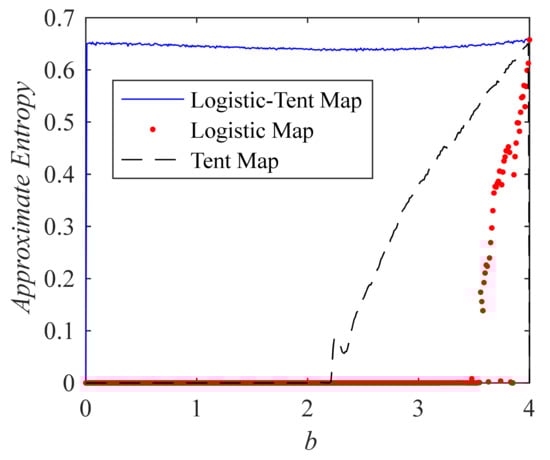
Figure 4.
Comparison of approximate entropy (ApEn) of sequences generated by three systems.
2.3.4. The Time-Series Diagram and Cobweb Graph of LTM System
The time-series diagram shows the variation law of time series with discrete time. Figure 5a shows the state values of two time series with an initial condition difference of 0.000001, indicating the strong sensitivity of time series to initial conditions.
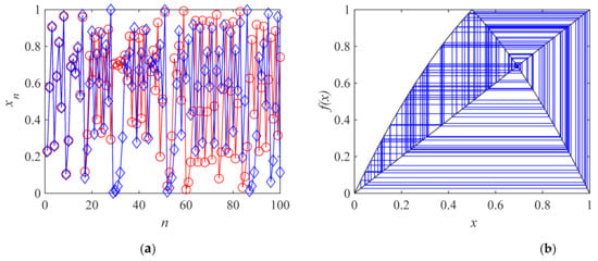
Figure 5.
The time-series diagram and cobweb graph of LTM system. (a) The time-series diagram; (b) the cobweb graph.
The cobweb diagram provides a powerful graphical means for studying the behavior of a dynamic system. It shows the long-term evolution law of system state values with time. Figure 5b shows the cobweb diagram formed by continuous iteration of the LTM system under a = 4, b = 1.3 and x0 = 0.1. It can be seen from Figure 5b that when a state initial value x0 is given, as a result, the system experiences an infinite number of non-repetitive chaotic orbits, which further confirms the chaotic behavior of system (4).
2.3.5. NIST Statistical Test Analysis
The NIST statistical test suite (version 2.1.1, National Institute of Standards and Technology, Gaithersburg, MD, USA) was used to evaluate the randomness of the bit sequence that was produced by the proposed system. The suite involves 15 tests which assess the randomness that might occur in a sequence. Each test result is converted to a p-value for judgement, and when applying the NIST test suite a significance level α = 0.01 is chosen for testing. If the p-value ≥ α, then the test sequence is considered to be pseudo-random. Setting 1000 different initial state values of the logistic tent map system (4) and iterating it 1,000,000 times for each initial state value generates 1000 sequences, 1 million bits each. The parameters used in the test are set as: a = 4, b = 0.35. For the first sequence, x0 = 0.11, and each time a 1,000,000 bits sequence is generated, the initial value of chaotic state variable increases by 0.001. Finally, each real number of state value x of the sequence is transformed into a binary number bx according to the following Algorithm 1:
| Algorithm 1. An algorithm for converting real numbers into binary numbers. |
| Intx = mod(floor(x × 1012),256); If Intx < 128 then bx = 1; Else bx = 0; End if |
Table 1 presents the results of NIST statistical test for 1000 sequences generated by the LTM, which indicates that the NIST test is effectively performed: All p-values among 1000 sequences used for testing are evenly distributed in the 10 subintervals, while the pass rate is also acceptable. The average pass rate is 99.01%, with one minimum pass rate of 98.1%. Experimental results show that the sequences generated by the logistic-tent map proposed in this paper have good pseudo randomness. Therefore, the compound chaotic system can be used as a pseudo-random number generator.

Table 1.
Results of NIST statistical test for 1000 sequences generated by the LTM.
3. The Proposed Image Encryption Scheme
First, in order to distinguish vectors and arrays from ordinary scalar variables easily in reading, some main symbols used in this paper are listed in Table 2.
Table 2.
Symbol description of variables used in this paper.
In this section, an image encryption scheme based on the LTM system is proposed. The scheme includes arbitrary T rounds of encryption processing, in which each round of encryption processing combines two kinds of operations, namely permutation and substitution. It realizes the scrambling and replacement processing of the input image simultaneously. The rapidity of the algorithm in this paper mainly comes from taking the whole row (or column) as the unit of operation processing, processing one row or one column instead of processing one pixel at one loop. This avoids dealing with pixels one by one circularly, which greatly reduces the number of loops. A row (or column) is actually a one-dimensional array, so every operation of the algorithm is an integral operation of the array. In this way, the loop of pixels can be avoided (reducing the number of loops is an important idea of this encryption algorithm).
3.1. The Encryption Process
Each round of the encryption process consists of the following three stages: (1) generating a modified chaotic sequence; (2) encryption processing row by row; (3) column-by-column encryption processing. The following describes the operation algorithm of each stage, respectively.
3.1.1. Generate a Modified Chaotic Sequence
At this stage, the chaotic system (4) is used to generate four modified chaotic sequences: X, Y, I, J. The detailed steps of the algorithm are described by Algorithm 2.
| Algorithm2. Generate the modified chaotic sequences. |
| Input: The number of rows M and columns N of the image to be encrypted, chaotic system parameters {x0, y0, a, b} and a positive integer N0. Output: Four sequences X, Y, I, J. |
Step 1: Iterate the system (4) with x0 as the initial value for (M + N0−1) times to generate a sequence x with the length of (M + N0). In order to improve the sensitivity of the intermediate key to the initial value, the first N0 values of the sequence are discarded, and the real chaotic sequence x = [x(1), x(2), …, x(M)]T with the final length of M is obtained. Iterate the system (4) for (N + N0−1) times with y0 as the initial value, and use the same method to generate the real-valued chaotic sequence y = [y(1), y(2), …, y(N)] with the final length of N.
Step 2: Use Equations (6), (7), (8) and (9) to obtain the sequences X = [X(1), X(2), …, X(M)]T, I = [I(1), I(2), …, I(M)]T, Y = [Y(1), Y(2), …, Y(N)] and J = [J(1), J(2), …, J(N)], respectively.
X = mod(floor(x × 106), 256),
Y = mod(floor(y × 106), 256),
[~, I] = sort(x),
[~, J] = sort(y).
Here, floor(x) is a function of rounding x, and the returned function value is the largest integer less than or equal to x; mod(x, 256) is the remainder obtained by dividing x by 256; [~, I] = sort(x) is to arrange the vector X in ascending order, and then get the position number of each element in the ordered sequence X’ in the original sequence X. These position number values {I (1), I (2), …, I (M)} constitute the sequence I, where the value of the element I(i) is the position value of the i-th element in the ordered sequence X’, I(i)∊{1, 2, …, M}. The meaning of J is similar to I. Here, i = 1, 2, …, M, j = 1, 2, …, N.
3.1.2. Row-by-Row Encryption Processing
In the row-by-row encryption processing stage, a row vector S(i) = [S(i)(1), S(i)(2), …, S(i)(j), …, S(i)(N)] related to the encrypted image content is used (superscript (i) stands for the i-th row). Before entering the row encryption stage (i = 0), the row vector S(i) takes the initial value S(0). The initial value S(0)(j) of any element in S(0) is equal to k times of the sum of all the elements in the j-th column of the current image P to be encrypted, which can be calculated with the following Equation (10), and the calculation principle can refer to Figure 6a.
where k is a positive integer greater than or equal to 1. By introducing parameter k, the change effect of pixel value P(i, j) can be amplified.
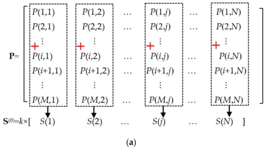
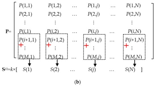
Figure 6.
A diagram for calculating the row vector S. (a) For calculating the row vector S(0), (b) for calculating the row vector S(i) (1 ≤ I < M).
When the i-th row of the input image is encrypted, the value of any element S(i)(j) in the vector S(i) is equal to k times of the sum of all elements whose row numbers are greater than i in the j-th column of the currently encrypted image P. The calculation principle of the vector S(i) is schematically shown in Figure 6b and can be expressed by the following Equation (11):
when the last row of the input image P is encrypted (i = M), all the element values in the vector S(i) are already equal to 0, that is, S(M) = [0, 0, …, 0].
Observing the general formula (11) of S(i), we can get the following relation:
That is:
From the relation between S(i) and S(i−1) described by Equation (12), we can get a method to increase the speed of calculating the vector S(i); that is, it is not necessary to directly calculate the sum of all elements after the i-th row by the cumulative sum method of the Equation (11) for the vector used in each row, but the recursive algorithm can be used instead. Therefore, the j-th element value of the vector S(i) corresponding to the current row (i-th row) can be obtained by subtracting k × P(i, j) from the j-th element value of the vector S(i) corresponding to the previous row (the (i-1)-th row). Only the element values of the initial vector S(0) must be directly calculated by the cumulative sum method of Equation (10). Therefore, the row vector S(i) needed to encrypt the i-th row can be calculated by the following algorithm: S(i)←S(i−1) − k × P(i, :). Here, P(i, :) represents a one-dimensional array composed of all elements in the i-th row of image P to be encrypted. Therefore, the Equation (12) with elements as operating units can be rewritten as the calculation Equation (13) with an array as operating units:
Executing Equation (13) is equivalent to executing Equation (12) for j = 1, 2, …, N in turn. In this way, a single row is treated as a single unit, turning an internal N times loop into a single loop.
The detailed operational steps of the row encryption phase are described in Algorithm 3 below.
| Algorithm 3. A row-by-row encryption algorithm that combines scrambling and substitution. |
| Input: Image matrix to be encrypted P = {P(i, j)|i = 1, 2, …, M; j = 1, 2, …, N}, x0, y0, a, b, C0 and N0. Output: Encrypted image matrix C = {C(i, j)|i = 1, 2, …, M; j = 1, 2, …, N}. |
Step 1: Call Algorithm 2 to generate four modified chaotic sequences: X, Y, I, J.
Step 2: Construct a row vector consisting of N identical constants C0: c = [C0, C0, …], and pre-allocate the storage space of M × N elements for the future encrypted image C.
Step 3: Get the initial row vector S = k × [S(1), S(2), …, S(j), …, S(N)] according to Equation (10), where S(j) is the sum of all pixel values in the j-th column in the image P.
Step 4: Sequentially execute the operations described by Equation (13) to (16) for i = 1, 2, …, M, respectively, and complete the encryption of the i-th row:
g = bitxor(Y, c).
An intermediate key sequence g is obtained from Equation (14), where g = [g(1), g(2), …, g(j), …, g(N)]. Executing Equation (14) is equivalent to performing the following operations for all j = 1, 2, ... , N, respectively: g(j) = bitxor(Y(j), c(j)).
C(I(i), :) = bitxor(mod(P(i, :) + S, 256), g).
Equation (15) completes the encryption processing of the i-th row P(i,:) and gets the pixel sequence C(I(i), :) of the I(i)-th row of the encrypted image. It can be seen that the i-th row of the image P is arranged to the I(i)-th row of the encrypted image C, where the position transformation occurs, that is, the scrambling effect of the position is produced. In addition, the pixel value of the I(i)-th row of the encrypted image C is different from the pixel value of the i-th row of the image P, that is, the substitution effect of pixel value is produced. Therefore, Equation (15) achieves both image row scrambling and pixel value substitution encryption.
c = C(I(i), :).
Equation (16) updates the value of row vector c to the currently encrypted image row C(I(i), :) in preparation for generating the intermediate key sequence g of the next row. Thus, it can be seen that the intermediate key sequence g used in the encryption of the (i + 1)-th row of image P is related to the ciphertext row C(I(i), :). This mechanism brings two advantages. First, it can produce the effect of diffusion, which makes the ciphertext sensitive to the change of plaintext (if only one pixel in the plaintext image P changes slightly, almost all pixels in the ciphertext image C will change); that is, the ciphertext is sensitive to plaintext, which can improve the ability of the algorithm to resist differential cryptanalysis. Secondly, the intermediate key sequence g is related to the image content, which allows the algorithm to resist the chosen-plaintext attack.
In order to describe the scrambling and substitution process of row-by-row encryption more intuitively, a simple example of an image with size of M = 2 rows and N = 4 columns is given in Figure 7. In Figure 7a, as the index vector I = [3, 1, 2] of the obtained row scrambling position, the row 1 of the image P is moved to the row I(1) of C, namely the row 3. Row 2 of P is moved to row I(2) of C, which is row 1; Row 3 of P is moved to row I(3) of C, which is row 2.
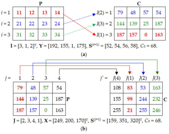
Figure 7.
The schematic diagram of one round of encryption. (a) The row-by-row encryption; (b) the column-by-column encryption.
3.1.3. Column-by-Column Encryption Processing
In the stage of column-by-column encryption, another S vector related to the encrypted image content is also used, but this vector is a column vector S = [S(1), S(2), …, S(i), …, S(M)]T. The initial value of any element S(i) in this vector is equal to k times of the sum of all the elements in the i-th row, and its calculation principle is the same as that described in Figure 6a. However, the sum is implemented for each row, which can be expressed by the following Equation (17) (compared with Equation (10)):
When encrypting the j-th column (1 ≤ j<N) of the input image, the value of any element S(j)(i) in the vector S(j) is equal to k times of the sum of all elements with column numbers greater than j in the i-th row, and its calculation principle is similar to that described in Figure 6b, but the sum is implemented for each row, which can be expressed by the following Equation (18) (compared with Equation (11)):
When the last column (j = N) of the input image is encrypted, the values of all elements in the vector S(j) will be 0, that is, S(j) = [0, 0, …, 0].
From Equation (18), the following relational expression (19) can be deduced:
That is
From the relation between S(j) and S(j−1) described by Equation (19), we can get a method to increase the speed of calculating the vector S(j); that is, it is not necessary to directly calculate the sum of all elements after the j-th column by the cumulative sum method of Equation (18) for the vector S(j−1) used in each column, but the following recursive algorithm can be used instead. Therefore, the i-th element value of the vector S(j) corresponding to the current column (j-th column) can be obtained by subtracting k × P(i, j) from the i-th element value of the vector S(j−1) corresponding to the previous column (the (j-1)-th column). Only the element values of the initial vector S(0) must be directly calculated by the cumulative sum method of Equation (17). Therefore, the column vector S(j) needed to encrypt the j-th column can be calculated by the following algorithm: S(j)←S(j−1)-k × P(:, j). Here, P(:, j), represents a one-dimensional array composed of all elements in the j-th column of image P to be encrypted. Therefore, the Equation (19) with elements as operating units can be rewritten as the calculation of Equation (20) with an array as operating units:
S(j) = S(j−1)-k × P(:, j).
Executing Equation (20) is equivalent to executing Equation (19) for i = 1, 2, …, M in turn. In this way, a single column is treated as a single unit, turning an internal M times loop into a single loop.
The detailed operational steps of the column encryption phase are described in Algorithm 4 below.
| Algorithm 4. A column-by-column encryption algorithm that combines scrambling and substitution. |
| Input: Image matrix to be encrypted P = {P(i, j)|i = 1, 2, …, M; j = 1, 2, …, N}, x0, y0, a, b, C0 and N0. Output: Encrypted image matrix C = {C(i, j)|i = 1, 2, …, M; j = 1, 2, …, N}. |
Step 1: Call Algorithm 2 to generate four modified chaotic sequences: X, Y, I, J.
Step 2: Construct a column vector consisting of M identical constants C0: c = [C0, C0, …]T and pre-allocate the storage space of M×N elements for the future encrypted image C.
Step 3: Get the initial column vector S = k × [S(1), S(2), …, S(i), …, S(M)] according to Equation (17), where S(i) is the sum of all pixel values in the i-th row in the image P.
Step 4: Sequentially execute the operations described by Equations (20) to (23) for j = 1, 2, …, N, respectively, and complete the encryption of the j-th column:
Equation (20) obtains the S vector at one time, which is equivalent to executing for all i = 1, 2, …, M, respectively: S(i) = S(i)-P(i, j).
h = bitxor(X, c).
An intermediate key sequence h is obtained from Equation (21), where h = [h(1), h(2), …, h(i), …, h(M)]. Executing Equation (21) is equivalent to performing the following operations for all i = 1, 2, …, M, respectively: h(i) = bitxor(X(i), c(i)).
C(:, J(j)) = bitxor(mod(P(:, j) + S, 256), h).
Equation (22) completes the encryption processing of the j-th column P(:, j), and gets the pixel sequence C(:, J(j)) of the J(j)-th column of the encrypted image. It can be seen that the j-th column of the image P is arranged to the J(j)-th column of the encrypted image C, where the position transformation occurs; that is, the scrambling effect of the position is produced. In addition, the pixel value of the J(j)-th column of the encrypted image C is different from the pixel value of the j-th column of the image P; that is, the substitution effect of pixel value is produced. Therefore, Equation (22) achieves both image column scrambling and pixel value substitution encryption.
c = C(:, J(j)).
Equation (23) updates the value of column vector c to the currently encrypted image column C(:, J(j)) in preparation for generating the intermediate key sequence h of the next column. Thus, it can be seen that the intermediate key sequence h used in the encryption of the (j + 1)-th column of image P is related to the J(j)-th column of ciphertext. Similar to row-by-row encryption, there are two effects at the same time: One is to move the column (the pixels in column j of the image P are moved to column J(j) of the encrypted image C) to produce the column scrambling effect; in addition, the intermediate key h is associated with the image content, which can make the algorithm have the ability to resist the chosen-plaintext attack. Figure 7b shows the process of column-by-column encryption.
After completing the above three processing stages, the input image undergoes a complete encryption round. In order to improve the security, multiple rounds of encryption can be repeated; that is, a total encryption round number parameter T is set in advance according to the needs, and before the above algorithms 2, 3 and 4 are called, the number of rounds counting variable r is initialized to 1. Then call the above algorithms 1, 2 and 3. After a certain round of encryption is completed, update the variable value of rounds counting variable r (increase it by 1): r = r + 1. If r < =T, take the currently obtained ciphertext matrix C as a new round of input image P to assign the current C matrix to P: P←C. Then repeat the above algorithms 2, 3 and 4 until the number of encryption rounds reaches T. The final output C matrix is the final ciphertext image. The larger the number of encryption rounds T, the more difficult it is to decipher the ciphertext and the higher the security, but the more time it takes to encrypt the image P. Therefore, the value of the T parameter should be determined according to actual demand.
3.2. Decryption Process
The decryption process is the reverse operation of the encryption process. Each round of decryption also includes three stages of operation, but the order of processing the three stages is: (1) generate the transformed chaotic sequence; (2) column-by-column decryption processing; (3) decrypt row by row.
3.2.1. Generate a Modified Chaotic Sequence
In this stage, four modified chaotic sequences X, Y, I and J are generated by chaotic system (4). The detailed steps of the algorithm are the same as Algorithm 2, except that the number of rows M and columns N of the image should be obtained according to the image C to be decrypted.
3.2.2. Column-by-Column Decryption Processing
The detailed operation steps of the column decryption phase are described by the following Algorithm 5.
| Algorithm 5. Column-by-column decryption algorithm. |
| Input: Image matrix to be decrypted C = {C(i, j)|i = 1, 2, …, M; j = 1, 2, …, N}, x0, y0, a, b, C0 and N0. Output: The decrypted image matrix P = {P(i, j)|i = 1, 2, …, M; j = 1, 2, …, N}. |
Step 1: Call Algorithm 2 to generate four modified chaotic sequences: X, Y, I, J.
Step 2: Initialize a column vector of length M: S = [0, 0, …, 0]T, and pre-allocate the storage space of M×N elements for the future decrypted image P.
Step 3: Processing is carried out from the last column to the second column; that is, for j = N, N-1, …,2, respectively, the decryption operation for the j-th column expressed by Equations (23), (21), (24) and (25) is carried out in turn:
P(:, j) = mod(bitxor(C(:, J(j)), h)-S, 256),
S = S+k×P(:, j).
Note that decryption Equation (24) is the inverse operation of encryption Equation (22), while Equation (25) is the inverse operation of Equation (20).
Step 4:j←1, For the first column, use Equations (26), (21), (24) and (25) to decrypt:
c = [C0, C0, …]T.
3.2.3. Row-by-Row Decryption Processing
The detailed operation steps of the row decryption phase are described by the following Algorithm 6.
| Algorithm6. Row-by-row decryption algorithm. |
| Input: Image matrix to be decrypted C = {C(i, j)|i = 1, 2, …, M; j = 1, 2, …, N}, x0, y0, a, b, C0 and N0. Output: The decrypted image matrix P = {P(i, j)|i = 1, 2, …, M; j = 1, 2, …, N}. |
Step 1: Call Algorithm 2 to generate four modified chaotic sequences: X, Y, I, J.
Step 2: Initialize a row vector of length N: S = [0, 0, …, 0], and pre-allocate the storage space of M×N elements for the future decrypted image P.
Step 3: Processing is carried out from the last row to the second row, that is, for i = M, M-1, …,2, respectively, the decryption operation for the i-th row expressed by Equations (16), (14), (27) and (28) is carried out in turn:
P(i, :) = mod(bitxor(C(I(i), :), g)-S, 256),
S = S+k×P(i, :).
Step 4:i←1, For the first row, use Equations (29), (14) and (27) to decrypt:
c = [C0, C0, …]T.
4. Experimental Test and Security Analysis
In this section, several classic test images are used for encryption experiments, and the performance of this encryption scheme is proved by the experimental test results. The experiment was completed on a PC equipped with Intel Core i7-9700 @ 3.00GHz processor, 16 GB RAM and MATLAB 2021a. The classic test images were from the image data set of USC-SIPI (https://ccia.ugr.es/cvg/dbimagenes/ (which can be accessed on 24 November 2021)). The key parameters used in the experiment were a = 4; b = 1.9; x0 = 0.23; y0 = 0.93; N0 = 57. Other parameters were set as: C0 = 73, m = 6, k = 5, T = 1.
4.1. Histogram Analysis
Image histogram describes the distribution frequency of gray values at all levels of the image. It visually shows whether the distribution number of pixel values of an image is uniform. Generally, the histogram distribution of meaningful images is uneven. However, the histogram of a good encrypted image should be flat and uniform so that attackers cannot obtain any useful information from the histogram of encrypted images. Figure 8 shows histograms of three test images and their corresponding encrypted images. It can be seen that the histograms of encrypted images are flat and evenly distributed.
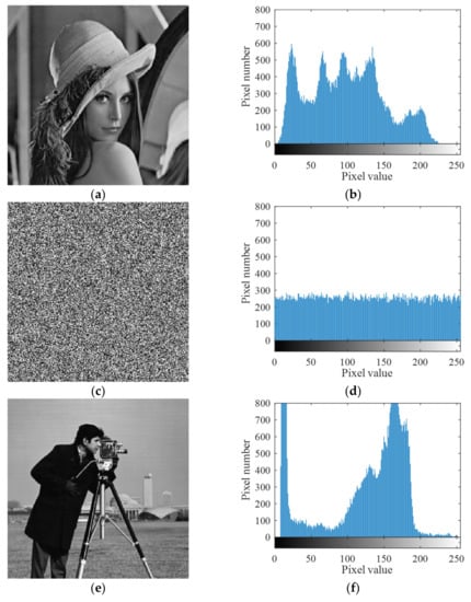
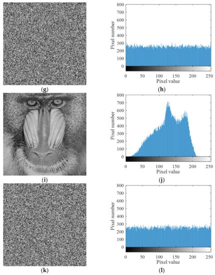
Figure 8.
Four test images and their ciphertext images and histograms. (a) Plaintext image Lena; (b) histogram of plaintext image Lena; (c) ciphertext image Lena; (d) histogram of ciphertext image Lena; (e) plaintext image cameraman; (f) histogram of plaintext image cameraman; (g) ciphertext image cameraman; (h) histogram of ciphertext image cameraman; (i) plaintext image baboon; (j) histogram of plaintext image baboon; (k) ciphertext image baboon; (l) histogram of ciphertext image baboon.
4.2. Correlation Analysis of Adjacent Pixels
The adjacent pixel values of meaningful plaintext images are usually highly correlated, so the correlation coefficient is close to 1. This strong correlation must be broken in the encryption process in order to destroy the relationship between the plaintext image and the encrypted image. The calculation equation of correlation coefficient is expressed by Equations (30)–(33):
We calculated the correlation coefficients between all adjacent pixel pairs in the horizontal, vertical and diagonal directions of a size of 256 × 256 gray image Lena and its ciphertext image. The results are listed in Table 3.
Table 3.
Comparing results of correlation coefficients for Lena (256 × 256).
From Table 3, it can be seen that the correlation coefficient of the original plaintext image is very close to 1, but the correlation coefficient of the encrypted image is very close to 0. Table 3 also lists the correlation coefficient results of the Lena image encrypted in several recently published algorithms. In contrast, our algorithm has certain advantages.
4.3. Information Entropy Analysis
Shannon information entropy is widely used to measure the randomness of distribution of a given information m. In image encryption, researchers use information entropy to quantify the information uncertainty in encrypted images. Shannon information entropy is calculated as follows:
When Equation (34) is used to calculate the image information entropy, represents the i-th gray value of L-level gray image (the gray level number of a common 8-bit gray image is L = 256), and represents the probability of occurrence of the i-th gray value. For ideal noise images with completely equal probability and random distribution of pixel values, the probability of occurrence of each gray level should be equal, that is, the are all constant 1/L = 1/256. By substituting this result into Equation (34), the ideal information entropy of 256 gray level images can be calculated as eight. If the information entropy of the encrypted image is closer to eight, it means that the more uniform its gray distribution is, the closer it is to the randomly distributed noise image and the more difficult it is to crack it. The information entropy values of several images encrypted by this algorithm are shown in Table 4. It can be seen from Table 4 that the information entropy of the encrypted image obtained by this algorithm is much larger than that of the original plaintext image. Moreover, in most cases, the information entropy of the ciphertext image obtained by this algorithm is higher than that of the algorithm in references, which shows that this algorithm has certain advantages.
Table 4.
Information entropy comparison of ciphertext images encrypted by different algorithms.
4.4. Sensitivity Analysis
(1) Sensitivity to plaintext
The robustness of encrypted images against chosen plaintext attacks and differential cryptanalysis is usually measured by the number of pixels change rate (NPCR) and the unified average change intensity (UACI) of pixel values. These metrics quantify the gap between encrypted images obtained from plaintext images and ciphertext images obtained from slightly modified plaintext images. NPCR and UACI are defined as follows:
where C(I, j) represents the pixel value of the ciphertext image obtained from the original plaintext image at coordinates (i, j), where it represents the pixel value of the ciphertext image obtained by encrypting after changing the lowest bit of a pixel of the original plaintext image at coordinates (i, j); M and N represent the height and width of the image, respectively. The definition of D(i, j) is as follows: if C(i, j) = C’(i, j), then D(i, j) = 1, otherwise, D(i, j) = 0. NPCR = 99.6094% and UACI = 33.4635% are the ideal expectations [13]. The larger the values of NPCR and UACI, the greater the difference between ciphertext images obtained from two plaintext images with slight difference, and the more sensitive (better) the algorithm is to plaintext.
In this experiment, first a plaintext image is encrypted for one round and the ciphertext image is recorded as C; then a pixel is randomly selected from the original image and is changed significantly, then the modified image is encrypted to obtain the ciphertext image C’ and 100 experiments are conducted. Finally, calculate the NPCR and UACI values between C and each C’. The average values of NPCR and UACI of 100 experiments are shown in Table 5 and Table 6, respectively.
Table 5.
Comparison of NPCR values of encrypted images (size 256 × 256).
Table 6.
Comparison of UACI values of encrypted images (size 256 × 256).
(2) Sensitivity to secret key
Key sensitivity is also one of the most basic security features of any cryptographic algorithm. On the one hand, the distribution of pixel values of encrypted images should sensitively change with the change of encryption keys, therefore, tiny differences in encryption keys must generate completely different password images. We encrypted a pair of the same plaintext images with randomly selected keys and slightly modified keys, and then tested the NPCR value between the two ciphertext images. The result showed that the NPCR value is very close to 99.61%, which indicates that the encryption process is sensitive to the key. On the other hand, the decryption of the ciphertext image must not use a slightly different key. Figure 9 shows the images decrypted with the correct key and the wrong keys which slightly deviated from the correct key, respectively. The results show that even if the decryption key is slightly different from the correct key, the original image cannot be restored, indicating that the decryption process is sensitive to keys. Therefore, the new cryptographic scheme proposed in this paper is sensitive to the key in the process of encryption and decryption.
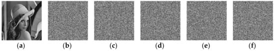
Figure 9.
Decrypted Lena images obtained by using different decryption keys. (a) Exactly the right key; (b) x0 is an error key with minimal error 10−15; (c) y0 is an error key with minimal error 10−15; (d) a is an error key with minimal error 10−15; (e) b is an error key with minimal error 10−15; (f) N0 is an error key with minimal error 1.
4.5. Key Space Analysis
The key parameters of the proposed algorithm are {a, b, x0, y0, N0}. Among them, {a, b, x0, y0} are double-precision real numbers and they can have 15 decimal digits, so each double-precision real number parameter has 1015 possible values. N0 is an integer between [1, 1000], and there are 103 values. Therefore, there are 1015 × 1015 × 1015 × 1015 × 103 ≈ 2209 key combinations. At present, the key space is greater than or equal to 2100, which can effectively resist violent attacks [37]. Therefore, the key space of this algorithm is large enough to effectively resist violent and exhaustive attacks.
4.6. Encryption Speed Test
In the proposed algorithm, there are M loops for row-by-row encryption and N loops for column-by-column encryption, which are two parallel loops, so the total number of loops is (M + N) and the time complexity of the algorithm is roughly expressed as O(M + N). The common image encryption algorithm takes a single pixel as the processing unit, so the number of loops of the algorithm is equal to the number of pixels, that is, (M × N) times, so the time complexity is O(M × N). The average time (average of 100 encryption experiments) spent by the proposed algorithm in one round of encryption is shown in the last column of Table 7 (unit: millisecond). Compared with other algorithms reported in the literature, this algorithm has obvious advantages in encryption speed.
Table 7.
Algorithm encryption speed test results (ms).
5. Conclusions
In this paper, a new one-dimensional compound chaotic map system was proposed. The system is composed of a logistic map and tent map. It has very wide range of chaotic parameters and strong chaotic behavior. It is very suitable for real-time image encryption based on chaos. Using some common tools in chaos theory, we analyzed the performance of the map. The results showed that the proposed map has good chaotic performance and strong chaotic behavior over a large range of parameter values. Furthermore, we designed a fast image encryption scheme with high security based on the new chaotic map. In this encryption scheme, the two processes of permutation and substitution are effectively combined to be realized simultaneously. The combination of these two phases makes the scheme faster and more secure than the traditional encryption structure, which handles permutation and substitution separately. Moreover, each loop of the encryption process takes one row or one column of an image as the processing unit rather than a single pixel as the processing unit, which greatly reduces the loop times of the algorithm, thus significantly improving the encryption speed. Simulation and experimental results show that the proposed image encryption scheme meets all the requirements of real-time applications.
Author Contributions
Conceptualization, S.Z. and C.Z.; methodology, W.Z. and X.D.; software, S.Z.; validation, S.Z., W.Z., X.D. and C.Z.; formal analysis, S.Z.; investigation, C.Z.; resources, W.Z.; data curation, S.Z.; writing—original draft preparation, S.Z.; writing—review and editing, C.Z.; visualization, X.D.; supervision, X.D. and W.Z.; project administration, W.Z.; funding acquisition, W.Z. All authors have read and agreed to the published version of the manuscript.
Funding
This research was funded by the Natural Science Foundation of Xinjiang Uygur Autonomous Region, grant number 2020D01C033.
Institutional Review Board Statement
Not applicable.
Informed Consent Statement
Not applicable.
Data Availability Statement
Exclude this statement.
Conflicts of Interest
The authors declare no conflict of interest.
References
- Liang, H.; Zhang, G.; Hou, W.; Huang, P.; Liu, B.; Li, S. A Novel Asymmetric Hyperchaotic Image Encryption Scheme Based on Elliptic Curve Cryptography. Appl. Sci. 2021, 11, 5691. [Google Scholar] [CrossRef]
- Li, Z.; Peng, C.; Tan, W.; Li, L. A Novel Chaos-Based Image Encryption Scheme by Using Randomly DNA Encode and Plaintext Related Permutation. Appl. Sci. 2020, 10, 7469. [Google Scholar] [CrossRef]
- El-Latif, A.A.A.; Abd-El-Atty, B.; Belazi, A.; Iliyasu, A.M. Efficient Chaos-Based Substitution-Box and Its Application to Image Encryption. Electronics 2021, 10, 1392. [Google Scholar] [CrossRef]
- Huang, L.-L.; Wang, S.-M.; Xiang, J.-H. A Tweak-Cube Color Image Encryption Scheme Jointly Manipulated by Chaos and Hyper-Chaos. Appl. Sci. 2019, 9, 4854. [Google Scholar] [CrossRef] [Green Version]
- Masood, F.; Ahmad, J.; Shah, S.A.; Jamal, S.S.; Hussain, I. A Novel Hybrid Secure Image Encryption Based on Julia Set of Fractals and 3D Lorenz Chaotic Map. Entropy 2020, 22, 274. [Google Scholar] [CrossRef] [PubMed] [Green Version]
- Moafimadani, S.S.; Chen, Y.; Tang, C. A New Algorithm for Medical Color Images Encryption Using Chaotic Systems. Entropy 2019, 21, 577. [Google Scholar] [CrossRef] [PubMed] [Green Version]
- Masood, F.; Driss, M.; Boulila, W.; Ahmad, J.; Rehman, S.U.; Jan, S.U.; Qayyum, A.; Buchanan, W.J. A Lightweight Chaos-Based Medical Image Encryption Scheme Using Random Shuffling and XOR Operations. Wirel. Pers. Commun. 2021, 1–28. [Google Scholar] [CrossRef]
- Belazi, A.; Abd El-Latif, A.A.; Belghith, S. A novel image encryption scheme based on substitution-permutation network and chaos. Signal Process. 2016, 128, 155–170. [Google Scholar] [CrossRef]
- Masood, F.; Boulila, W.; Ahmad, J.; Arshad; Sankar, S.; Rubaiee, S.; Buchanan, W.J. A Novel Privacy Approach of Digital Aerial Images Based on Mersenne Twister Method with DNA Genetic Encoding and Chaos. Remote Sens. 2020, 12, 1893. [Google Scholar] [CrossRef]
- May, R.M. Simple mathematical models with very complicated dynamics. Nature 1976, 261, 459–467. [Google Scholar] [CrossRef]
- Lambic, D. Security analysis and improvement of a block cipher with dynamic S-boxes based on tent map. Nonlinear Dynam. 2015, 79, 2531–2539. [Google Scholar] [CrossRef]
- Belazi, A.; El-Latif, A.A.A. A simple yet efficient S-box method based on chaotic sine map. Optik 2017, 130, 1438–1444. [Google Scholar] [CrossRef]
- Talhaoui, M.Z.; Wang, X.; Midoun, M.A. A new one-dimensional cosine polynomial chaotic map and its use in image encryption. Vis. Comput. 2021, 37, 541–551. [Google Scholar] [CrossRef]
- Ponuma, R.; Amutha, R. Compressive sensing based image compression-encryption using Novel 1D-Chaotic map. Multimedia Tools Appl. 2018, 77, 19209–19234. [Google Scholar] [CrossRef]
- Talhaoui, M.Z.; Wang, X. A new fractional one dimensional chaotic map and its application in high-speed image encryption. Inf. Sci. 2021, 550, 13–26. [Google Scholar] [CrossRef]
- Zhu, S.; Wang, G.; Zhu, C. A Secure and Fast Image Encryption Scheme based on Double Chaotic S-Boxes. Entropy 2019, 21, 790. [Google Scholar] [CrossRef] [Green Version]
- Zhu, H.; Zhang, X.; Yu, H.; Zhao, C.; Zhu, Z. A Novel Image Encryption Scheme Using the Composite Discrete Chaotic System. Entropy 2016, 18, 276. [Google Scholar] [CrossRef] [Green Version]
- Ramasamy, P.; Ranganathan, V.; Kadry, S.; Damaševičius, R.; Blažauskas, T. An image encryption scheme based on block scrambling, modified zigzag transformation and key generation using enhanced logistic-tent map. Entropy 2019, 21, 656. [Google Scholar] [CrossRef] [Green Version]
- Gupta, M.; Gupta, K.K.; Khosravi, M.R.; Shukla, P.K.; Kautish, S.; Shankar, A. An intelligent session key-based hybrid lightweight image encryption algorithm using logistic-tent map and crossover operator for internet of multimedia things. Wirel. Pers. Commun. 2021, 1–22. [Google Scholar] [CrossRef]
- Tong, X.J.; Wang, Z.; Zhang, M.; Liu, Y.; Xu, H.; Ma, J. An image encryption algorithm based on the perturbed high-dimensional chaotic map. Nonlinear Dynam. 2015, 80, 1493–1508. [Google Scholar] [CrossRef]
- Pak, C.; Huang, L. A new color image encryption using combination of the 1D chaotic map. Signal Process. 2017, 138, 129–137. [Google Scholar] [CrossRef]
- Dou, Y.; Li, M. Cryptanalysis of a New Color Image Encryption Using Combination of the 1D Chaotic Map. Appl. Sci. 2020, 10, 2187. [Google Scholar] [CrossRef] [Green Version]
- Zhu, C.; Wang, G.; Sun, K. Improved Cryptanalysis and Enhancements of an Image Encryption Scheme Using Combined 1D Chaotic Maps. Entropy 2018, 20, 843. [Google Scholar] [CrossRef] [PubMed] [Green Version]
- Hua, Z.; Zhou, Y. Image encryption using 2D Logistic-adjusted-Sine map. Inf. Sci. 2016, 339, 237–253. [Google Scholar] [CrossRef]
- Feng, W.; He, Y.; Li, H.; Li, C. Cryptanalysis and Improvement of the Image Encryption Scheme Based on 2D Logistic-Adjusted-Sine Map. IEEE Access 2019, 7, 12584–12597. [Google Scholar] [CrossRef]
- Wang, X.; Liu, C.; Zhang, H. An effective and fast image encryption algorithm based on Chaos and interweaving of ranks. Nonlinear Dynam. 2016, 84, 1595–1607. [Google Scholar] [CrossRef]
- Azimi, Z.; Ahadpour, S. Color image encryption based on DNA encoding and pair coupled chaotic maps. Multimed. Tools Appl. 2019, 79, 1727–1744. [Google Scholar] [CrossRef]
- Fath Allah, M.I.; Eid, M.M. Chaos based 3D color image encryption. Ain Shams Eng. J. 2019, 11, 67–75. [Google Scholar] [CrossRef]
- Malik, D.S.; Shah, T. Color multiple image encryption scheme based on 3D-chaotic maps. Math. Comput. Simul. 2020, 178, 646–666. [Google Scholar] [CrossRef]
- Hua, Z.; Yi, S.; Zhou, Y. Medical image encryption using high-speed scrambling and pixel adaptive diffusion. Signal Process. 2018, 144, 134–144. [Google Scholar] [CrossRef]
- Belazi, A.; Talha, M.; Kharbech, S.; Xiang, W. Novel Medical Image Encryption Scheme Based on Chaos and DNA Encoding. IEEE Access 2019, 7, 36667–36681. [Google Scholar] [CrossRef]
- Banu, S.A.; Amirtharajan, R. A robust medical image encryption in dual domain: Chaos-DNA-IWT combined approach. Med. Biol. Eng. Comput. 2020, 58, 1445–1458. [Google Scholar] [CrossRef]
- Yan, X.; Wang, X.; Xian, Y. Chaotic image encryption algorithm based on arithmetic sequence scrambling model and DNA encoding operation. Multimed. Tools Appl. 2021, 80, 10949–10983. [Google Scholar] [CrossRef]
- Alawida, M.; Samsudin, A.; Sen Teh, J.; Alkhawaldeh, R.S. A new hybrid digital chaotic system with applications in image encryption. Signal Process. 2019, 160, 45–58. [Google Scholar] [CrossRef]
- Zhu, C. A novel image encryption scheme based on improved hyperchaotic sequences. Opt. Commun. 2012, 285, 29–37. [Google Scholar] [CrossRef]
- Liu, W.; Sun, K.; Zhu, C. A fast image encryption algorithm based on chaotic map. Opt. Lasers Eng. 2016, 84, 26–36. [Google Scholar] [CrossRef]
- Alvarez, G.; Li, S. Some basic cryptographic requirements for chaos-based cryptosystems. Int. J. Bifurc. Chaos 2006, 16, 2129–2151. [Google Scholar] [CrossRef] [Green Version]
Publisher’s Note: MDPI stays neutral with regard to jurisdictional claims in published maps and institutional affiliations. |
© 2021 by the authors. Licensee MDPI, Basel, Switzerland. This article is an open access article distributed under the terms and conditions of the Creative Commons Attribution (CC BY) license (https://creativecommons.org/licenses/by/4.0/).