Featured Application
This paper proposes an object detection and tracking system that can count vehicles, estimate the velocity of vehicles, and provide traffic flow estimations for traffic monitoring and control applications.
Abstract
This paper proposes a neural network that fuses the data received from a camera system on a gantry to detect moving objects and calculate the relative position and velocity of the vehicles traveling on a freeway. This information is used to estimate the traffic flow. To estimate the traffic flows at both microscopic and macroscopic levels, this paper used YOLO v4 and DeepSORT for vehicle detection and tracking. The number of vehicles passing on the freeway was then calculated by drawing virtual lines and hot zones. The velocity of each vehicle was also recorded. The information can be passed to the traffic control center in order to monitor and control the traffic flows on freeways and analyze freeway conditions.
1. Introduction
Self-driving cars are one of the most important areas of study in the field of artificial intelligence. By combining the data from internal and external sensors, and accurately detecting the surrounding objects, driving safety can be improved. In recent years, object detection in computer vision has been developed, including detecting nearby vehicles, pedestrians, and obstacles, and measuring the distances between them, recognizing traffic signals and signs for self-driving cars, and counting the amounts of vehicles passing on a highway. Fully-Connected Network (FCN) techniques to detect and localize objects in the form of 3D boxes from range scan data have been developed.
This paper focuses on various methods of object detection and tracking for vehicles on a highway. These were applied to estimate regional traffic flow, detect objects, and measure their position and velocity. To achieve this, a neural network is proposed to estimate surrounding traffic flow. It is combined with processes of moving object detection and can calculate the relative position and velocity of moving objects. By individually identifying three lanes in each direction (northbound and southbound), and classifying and counting the vehicles, the vehicle density of each lane can be calculated correctly. This newly proposed method can provide real-time accurate data for traffic control and analysis.
In Taiwan, traffic jams during commuting hours are a tremendous problem, especially for such a highly populated and urbanized small island. The main purpose of this study was to provide data to the Traffic Control Center to reduce the occurrence of traffic jams by applying artificial intelligence techniques. Existing models for vehicle detection and tracking sometimes have the problem of repeat counting due to inconsistencies in object tracking. To solve this problem, our model introduced “virtual lines” and “hot zones” (detailed in Section 3.3.2) to accurately count the number of vehicles passing in each lane of the section of freeway. The benefit of adding a hot zone is that when a vehicle moves close to the virtual line, it can be tracked more accurately, and repeat counting is avoided. A deep learning procedure using a neural network technique was designed for estimating the velocity of vehicles. By providing the data obtained from our system to the Traffic Control Center, each car, self-driving or not, can be recommended the optimal route and, thus, the traffic situation can be improved.
This paper has three main features. First, the traffic flow counted by the Freeway Bureau, the Ministry of Transportation and Communications (MOTC), Taiwan, uses Electronic Toll Collection (ETC) sensors to count cars; however, this misses cars that do not have the ETC installed. In this study, object detection and tracking were used to count vehicles and estimate velocity, which not only solves the aforementioned problem, but also reduces costs. Second, in this study, the traffic flow of each lane was calculated individually, rather than simply in two directions. Third, our technique is able to represent different colors in each lane according to the velocity level. These features are beneficial to traffic flow monitoring and control by the Freeway Bureau, MOTC, Taiwan, especially in situations of heavy traffic, such as those seen during commuting hours and holidays.
2. Related Works
Currently, deep learning is a popular academic and technological topic which is applied in various AI techniques, including those associated with self-driving cars and transportation. Traffic flow monitoring using video has been applied to different traffic scenes, such as city roads, highways, and intersections [,]. Deep learning research applied to solve traffic flow predictions has also developed in recent years. In the 21st century, researchers proposed a deep learning-based traffic flow prediction method to identify various cars running on the highway. For example, the software tools developed by Y. LV et al. used the stack autoencoder (SAE) approach to represent traffic flow features maps for predictions. The greedy layer-wise unsupervised learning algorithm was applied to pretrain the network before the model’s parameters were updated using a fine-tuning process to improve the prediction [].
There are various other deep learning models that were developed to predict traffic flow. For example, N.G. Polson et al. proposed a deep learning model to predict short-term traffic flow []. W.S. McCulloch developed a model which is a combination of a linear model with L1 regularization and some tanh layers []. V. Minh et al. designed a deep learning predictor that takes an input vector and output via different layers []. They developed a linear model using previous measurements to provide a forecast.
The techniques for object detection and object tracking are important for vehicle counting. For object detection, there are object detectors such as YOLO, Faster R-CNN, SSD, etc. YOLO is a state-of-the-art, real-time object detection system [,]. This object detection method proposed by Joseph Redmon et al. used regression methods to calculate the bounding box and the related classification probability of the detected objects. A single neural network is used to predict the bounding box and classification probability directly from the complete image in one evaluation. Since the entire detection is a single network, the end-to-end detection performance can be directly optimized []. YOLO can solve the special regression problem of object detection frames, and can identify the object and predict the bounding box simultaneously. Therefore, YOLO is one of the most widely used object detection tools, and is especially powerful in high real-time detection tasks. Moreover, newer versions have been developed to improve detection performance. YOLO v2 has a higher accuracy, has a higher efficiency (by adding a batch normalization layer into the convolutional neural networks), and has a high-resolution classifier. YOLO v3 uses multi-label classification, in which an object may belong to multiple categories at the same time. YOLO v3 replaces the softmax function with an independent logistic function to calculate the probability that the input belongs to a specific label. In addition, instead of using the mean square error to calculate the classification loss, YOLO v3 uses the two-class cross-entropy loss for each category. This approach also reduces the computational complexity brought about by the softmax function. YOLO v3 uses DarkNet-53 as the main backbone of the convolutional neural networks to extract features from the input image, which has a better efficiency and detection performance than other backbones []. The architecture of DarkNet-53 is shown in Table 1.

Table 1.
The architecture of DarkNet-53 [].
YOLO v4 was released in April 2020 and has a higher accuracy and efficiency for object detection, with reduced hardware requirements []. YOLO v4 established an efficient and powerful object detection model, verified the influence of the state-of-the-art Bag-of-Freebies and Bag-of-Specials object detection methods in the training process, and improved the techniques of optimizing the network during training and testing. YOLO v4 uses CSPDarknet53, a combination of Darknet53 and the Cross Stage Partial Network (CSPNet), [] as the main backbone of convolutional neural networks.
The procedure of object tracking generally includes the following steps []: first, input the video and execute the object detectors, such as YOLO, Faster R-CNN, or SSD, to detect the objects and obtain their detection frames. Then, obtain all the corresponding targets from the detection frames and extract their features, including apparent features and/or motion features. Thereafter, calculate the similarity between these objects in adjacent frames. Finally, after linking the same objects together, assign different objects with different IDs.
For object tracking, SORT (Simple Online and Realtime Tracking) is combined with the Kalman filter and the Hungarian Algorithm, which enhances the efficiency of multiple object tracking. The Kalman filter algorithm is divided into two processes: prediction and update. The algorithm defines the motion state of the target as eight normally distributed vectors. When the target moves, the target frame position and the speed of the current frame are predicted based on the target frame and the speed of the previous frame. The predicted value and the observed value are obtained, the two normal distribution states are linearly weighted, and the current state of the system prediction is obtained. In the main multiple object tracking step, the similarity is calculated and the similarity matrix of the two frames before and after is obtained. The Hungarian algorithm solves the real matching goal of the two frames before and after solving this similarity matrix []. The object tracking procedure of SORT is shown in Figure 1.
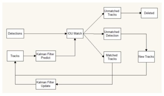
Figure 1.
Object tracking procedure of SORT [].
DeepSORT was developed from SORT. Information about the exterior of the objects was added in order to match objects in adjacent frames. The procedure of DeepSORT is as follows: first, the Kalman filter is used to predict the trajectory. Then, the Hungarian algorithm is used to match the predicted trajectory with the detections in the current frame (cascade matching and IOU matching). Thereafter, the Kalman filter is updated. DeepSORT can be applied in Multiple Object Tracking (MOT), which can assign each vehicle with different IDs. The object tracking procedure of DeepSORT is shown in Figure 2.
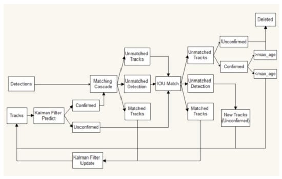
Figure 2.
Object tracking procedure of DeepSORT [].
Z. Wang et al. proposed a multiple object tracking system that has a detection model for target localization and an appearance embedding model for data association []. A. Fedorov et al. applied a faster R-CNN detector and a SORT tracker in traffic flow estimation with data from a camera []. The application of YOLO and DeepSORT can be used in many multiple object tracking scenarios other than just traffic [], including crowd control [] and detecting and tracking moving obstacles [].
This study applied artificial intelligence to improve traffic flow monitoring methods. Traffic flow prediction is one of the most important topics for self-driving cars, and various methods and algorithms have been developed in the past decade to improve route guidance for cars and assist traffic management and control. Neural network models have also been developed for traffic flow prediction. By identifying vehicles from traffic videos with artificial neural networks (ANNs), the methods proposed herein can help to improve highway traffic jams in Taiwan.
3. Methods
3.1. Process and Flow Chart
The complete process is shown as a flow chart in Figure 3. After inputting the video, our system detects the vehicles using YOLO v4, and then tracks the vehicles using DeepSORT. Finally, the number of vehicles that passed through each lane and the velocity of each vehicle are calculated.
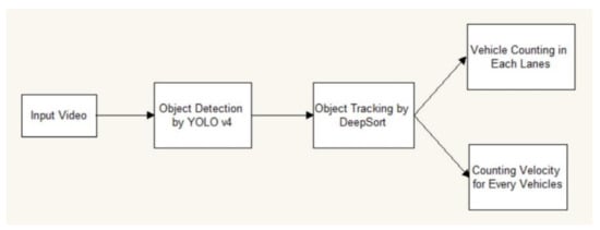
Figure 3.
Flow chart of the whole process.
3.2. Traffic Flow Calculation Model
Here are some fundamental quantities for traffic flow []: density is defined as the number of vehicles per unit length. The speed and positions of the n-th vehicle are denoted as and , respectively. Flow rate f is the number of vehicles passing a fixed position per unit time (for example, 1 h). Time mean speed is the average vehicle speeds in the fixed position over time, and space mean speed is the average vehicle speeds over a hot zone in a fixed time. Bulk velocity is defined as the ratio of flow rate to density, i.e., .
The traffic flow can be described microscopically and macroscopically, as proposed by B. Seibold []. The microscopic description of traffic flow was used to characterize each vehicles’ behavior, was applied in many car-following models (e.g., the intelligent driving model), and was used to facilitate a self-driving car’s decision of keeping in the same lane or switching to other lanes, to avoid backing up.
For the microscopic description, there are individual trajectories: the vehicle position equation:, the vehicle velocity equation: v1(t), v2(t), …, vn(t), and the acceleration equation: [].
For microscopic traffic models, two models are required: the “follow the leader” model: accelerate/decelerate towards the velocity of the vehicle ahead of the self-driving car itself. If the position and velocity of the vehicle ahead is p2 and v2, then according to the “follow the leader” model [] the acceleration is expressed as:
The “optimal velocity” model: accelerate/decelerate towards an optimal velocity that depends on your distance to the vehicle ahead. Then, the acceleration according to this model should be:
By combining both models, the acceleration of the self-driving car can be obtained in the following equation:
On the other hand, the macroscopic description of traffic flow is usually lane aggregated; however, multi-lane models can also be formulated. The macroscopic description of traffic flow is also good for estimation and prediction, and for the mathematical analysis of emergent features. It can examine larger portions of highway, judge whether the traffic in each section is convenient or heavy, and assist navigation and determine the path planning for a car.
Macroscopic descriptions are based on field quantities, including the vehicle density , velocity field , and flow-rate field , where p is the position on the road and t is time [].
To set up macroscopic traffic models, the following equations are needed: the number of vehicles in the section interval c to d can be obtained from vehicle density as follows:
Traffic flow rate (flux):
Change in the number of vehicles equals inflow f(c) minus outflow f(d) dynamically as follows:
This equation holds for any choice of c and d:
The microscopic view of traffic flow was studied in this study, and the macroscopic view of traffic flow will be studied in the future. Both descriptions have their own significance and usage.
3.3. Object Identification and Vehicle Tracking
3.3.1. Pretrain and Retrain for Object Identification
Our inputs were obtained from the MP4 videos taken at several fixed points on the National Freeway No.1 from the Freeway Bureau, MOTC in Taiwan. In the process of object detection, we used YOLO v4 to identify objects in every frame (with approximately 2000 to 9000 frames per video). The model was pretrained using the Coco dataset, and then retrained with our own picture data from classified vehicles, whose categories corresponded to the Coco dataset [,]. In each frame, the bounding boxes of all vehicles were labelled and classified. In addition, the centers of each vehicle were identified and the distances between them were measured. Through a visual inspection of the outcome, the vehicles were correctly identified and correctly classified into cars, buses, and trucks: the three relevant categories of vehicles for the Taiwanese freeway.
3.3.2. Object Tracking by Drawing Virtual Lines and Hot Zones
In this study, we used DeepSORT to track the objects (vehicles) identified by YOLO v4. In brief, DeepSORT first uses the Kalman filter to predict the trajectories of objects from previous frames. Then, it uses the Hungarian algorithm to match the predicted trajectories with the detected objects in the current frame (using cascade matching and IOU matching). Thereafter, it updates the Kalman filter for further predictions []. By executing DeepSORT, we were able to calculate the similarities between the apparent features and/or motion features of objects in adjacent frames, link the same objects together, assign different IDs to different objects, and track the objects throughout the video.
In order to calculate lane-specific traffic flows, we drew a virtual line in each direction of the highway (Figure 4) in the images and counted the number of vehicles (as defined by the centers of their bounding boxes) passing the lines in each lane. As a result, a vehicle that changed lanes in the video would only be counted in one of the lanes, as determined by its location while passing through the virtual line. There are six lanes on the sections of National Freeway No.1 in which the videos were taken (Figure 5). The input video’s resolution was 1920 × 1080 pixels, with 30 frames per second.
During object tracking, the system sometimes lost track of an object for a few frames and then recaptured it; sometimes it was identified as a different object and reassigned with a different ID. Such object tracking inconsistencies can cause the system to become unreliable, as a result of repeated counting of vehicles and confusion in speed calculations (in Section 3.3.3). Therefore, we modified the algorithm by adding hot zones in the vicinity of virtual lines (Figure 4), and only performed object tracking when the center was within the hot zones. The introduction of hot zones improved the accuracy of vehicle tracking and the subsequent calculations.

Figure 4.
Virtual lines and hot zones of the inner lanes of both directions (conceptualization).

Figure 5.
Sample image of the video taken on National Freeway No.1.
3.3.3. Estimation of Velocities of Each Vehicle
As shown in Figure 6, when drawing two virtual lines separated by a fixed distance (e.g., 20 m) in a bigger hot zone and obtaining the two time points through which a vehicle passes the two virtual lines (t1 and t2) using the aforementioned object tracking technique, the velocity of the vehicle can be calculated as follows:
where d is the fixed distance.
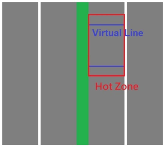
Figure 6.
Two virtual lines and hot zone for the velocity calculation (conceptualization).
The parameters can be acquired as follows:
p1, p2, …, pn: the positions of vehicles;
v1, v2, …, vn: the velocities of vehicles.
After inputting these data, the velocities of vehicles could be classified into five levels as defined by the Freeway Bureau, MOTC, Taiwan (Table 2):
Table 2.
Levels of speed classification.
Similarly, we were able to classify each lane into different speed levels from the average speed of vehicles, and color-code the lanes for visualization.
4. Experiments
The results from digital image processing, object detection, and object tracking were as follows: we obtained accurate vehicle counts for both the northbound and southbound directions, and for each lane separately. Moreover, the velocities of all vehicles were estimated.
4.1. Digital Image Processing
The video taken on National Freeway No.1 was processed into an MP4 video and was used as the input for our system.
4.2. Object Detection Results
Our model using YOLO v4, trained with the Coco dataset and our own picture dataset, was able to identify all the vehicles on the freeway and perform accurate classifications (Figure 7).
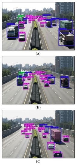
Figure 7.
Object detection results on the video taken on National Freeway No.1 (a–c). The identified vehicles were wrapped with their respective bounding boxes. The colors of the bounding boxes represent the categories of the vehicles: cars (magenta), trucks (blue), and buses (green).
4.3. Vehicle Counting in Both Northbound and Southbound Directions
By adding virtual lines and hot zones to both the northbound and southbound sides of the freeway, the vehicles that entered into the hot zones could be tracked accurately and, thus, we were able to correctly count the number of vehicles passing through the virtual line (Figure 8), which in turn yielded the flow rate (the number of vehicles passing through per unit time) of the section of the freeway in any given time interval.
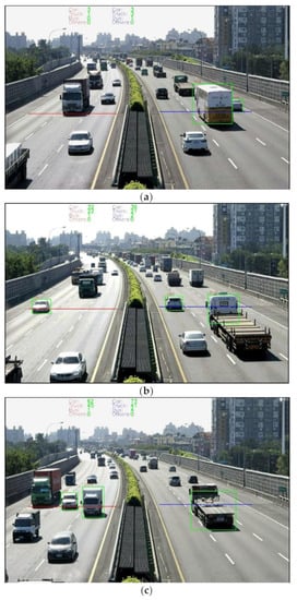
Figure 8.
The results of vehicle counting in both the northbound and southbound lanes from the video taken on National Freeway No.1 (a–c). The red line represents the virtual line in the northbound direction, while the blue line represents the virtual line in the southbound direction. Note that only the vehicles approaching the virtual lines were tracked (marked with green boxes).
4.4. Vehicle Counting in Each Lane in Both Northbound and Southbound Directions
The hot zones and virtual lines that we introduced also allowed us to calculate the vehicle count and the flow rate for each lane individually (Figure 9). Each vehicle was only counted once, in the lane in which it passed through the virtual line.
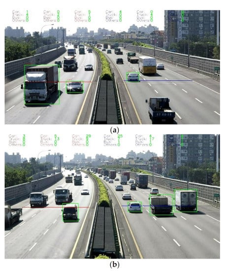
Figure 9.
The results of vehicle counting in both the northbound and southbound lanes from the video taken on National Freeway No.1 (a,b). The red line represents the connected virtual lines in the three northbound lanes, while the blue line represents the connected virtual lines in the three southbound lanes. The green boxes mark the vehicles tracked in the hot zones.
The vehicle counting results were illustrated in Table 3. We compared the vehicle counts in each lane using a visual inspection and the object detection of our system for three min. The errors were caused by double-labeling large trucks (e.g., trailer trucks, container cars), erroneously counting vehicles in the adjacent lane (Lane 2 to Lane 1; Lane 5 to Lane 6), and large trucks blocking small cars from the camera.
Table 3.
Vehicle counting results (in three min).
4.5. Velocity Estimation
The velocity of each vehicle on the freeway was calculated using Equation (8), the results are shown in Figure 10.
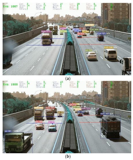
Figure 10.
Velocity estimation in the video taken on National Freeway No.1 (a,b).
4.6. Velocity Level
As the velocities of the vehicles passing through the lane were calculated, the color of the virtual line changes to represent the velocity level of the lane according to Table 2, the results are shown in Figure 11. The colors representing Level 1 to 5 are purple, red, orange, yellow, and green, respectively.
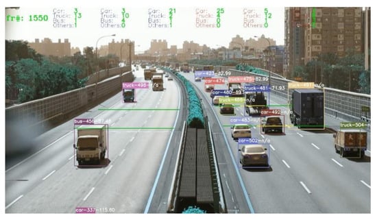
Figure 11.
The velocity level of each lane in the video taken on National Freeway No.1.
5. Discussion
In this study, we trained a YOLO v4 model for object detection. It was able to successfully identify all vehicles in the input video, and classify them into cars, buses, and trucks. Thereafter, we used DeepSORT for multi-object tracking. It was able to track these vehicles frame-to-frame and trace their individual trajectories.
Furthermore, we introduced virtual lines and hot zones into our DeepSORT-based tracking system, which improved the accuracy of lane-specific vehicle counts (mostly as a result of avoiding duplicates) and facilitated the calculation of individual vehicle velocities. These improvements, in turn, enabled the accurate estimation of the lane-specific flow rate and average speed. The visualization of the color-coded velocity level in each lane indicated the condition of each lane.
There are several potential applications for our system. First of all, if our system is linked to the Traffic Control Center, we can obtain real-time information, such as the number of different types of vehicles, the lane-specific flow rate, the lane-specific average speed, etc., which will be able to provide detailed real-time monitoring and analysis of traffic conditions throughout the highway system, and play an important part in decision-making or even law-enforcement processes for the authorities. In Taiwan, video cameras are set at most sections in our National Highway System. Therefore, our system could be implemented at a low cost and provide more accurate and detailed traffic monitoring than the Freeway Bureau’s (MOTC) current ETC-based monitoring system, which can only provide the overall flow rate for ETC-enabled vehicles. The Freeway Bureau, MOTC, spent considerable funds on assembling ETC for vehicle counting; however, our object detection and tracking system can be simply implemented using a camera, which will both save funds for vehicle counting and enhance the system by adding the function of vehicle speed estimation. Since our system is less costly and requires less maintenance than ETC-based or induction-based traffic monitoring systems, it would also be more feasible for developing countries that lack the adequate infrastructure.
In addition, the real-time information acquired from our system could be transmitted to individual drivers or self-driving cars in order to help them make decisions, such as staying in the same lane or switching to another lane if approaching a partially congested section of the freeway. When integrated with navigation systems, it would aid in recommending the optimal route to each vehicle.
Moreover, if our system were set up throughout the entire freeway, the abundant data concerning individual vehicles obtained by our system, such as their type, speed, time in a section, and the lanes used, would be helpful for the analysis of road occupants’ habits and could be used to build traffic and prediction models.
In this study, we further simplified the classifications of detected objects to cars, buses, and trucks (any other object would be classified as “others”), because these are the only three types of vehicles that appear on a Taiwanese freeway. In fact, it is well within YOLO’s ability to provide a more detailed and broader range of classifications. When coupled with our real-time lane-specific traffic statistics, this extended system is capable of both congestion detection and identifying the cause of congestion (e.g., if an animal appeared on the freeway, or if a scooter illegally entered the freeway).
This paper is concerned with vehicle detection, vehicle tracking, and speed estimation. The proposed approach improves upon existing approaches. For example, two papers in our literature review concerning the applications of YOLO and DeepSORT [,,,] were related to traffic flow estimation. In these, A. Federov et al. only counted vehicles passing the crossroad in different directions, [] and A. Santos et al. only counted vehicles on Brazilian roads []. In this study, we not only counted vehicles passing on the freeway in each lane, but also calculated the velocity of these vehicles, and the velocity level in each lane. Therefore, our system has more functional applications for traffic monitoring and control. In addition, our system used YOLO v4 for object detection, which has a higher accuracy and efficiency than YOLO v3, which A. Santos et al. used. Our system used DeepSORT for object tracking, which added the Deep Association Metric to SORT and enabled objects with different IDs to be assigned. Thus, our system can perform Multiple Object Tracking (MOT) better than SORT, which A. Federov et al. used.
Because we defined the position of a vehicle as the center of its bounding box, if the curvature of the road surface is too large or the size of the vehicle is too large, that center point can sometimes fall in the adjacent lane, and the vehicle is erroneously counted. This problem only affected the lane-specific estimations, but not the estimations of the overall direction.
6. Conclusions and Future Work
In recent years, deep learning techniques for optimizing object detection and tracking have developed rapidly and have been applied to human and vehicle traffic flows [,]. To our knowledge, this study was the first to introduce virtual lines and hot zones to a deep learning object detection and tracking system for lane-specific vehicle counting and velocity estimation.
Our contributions to traffic flow estimation are detailed in the third to fifth paragraph of the Discussion Section. Briefly, the contributions are as follows: the system proposed in this paper can provide detailed real-time information including the number of vehicles passing in each lane of the section of freeway, the vehicle types, and the velocities of these vehicles. Such information can be provided to the authorities for traffic monitoring and control, shared with individual vehicles (including self-driving cars) for navigation, and analyzed by official or academic institutions for traffic modeling and prediction. Since the system proposed in this paper can be simply implemented using video cameras set on the freeway, its efficiency, low cost, and high data quality are superior to ETC-based traffic monitoring systems for traffic counting and analysis.
In the future, we will continue to improve the prediction accuracy, especially that of lane-specific counting. We will also study techniques concerning the macro-view of traffic flow, and we hope to develop an attention model that can automatically describe the complete traffic situation on a larger scale.
The wireless sensor networks (WSNs) are widely applied, and security has become a major concern for WSN protocol designers []. All detection schemes are subject to cybersecurity attacks. Main cyber vulnerabilities include internet exposition, interface/password breaches, update lack, low segregation, weakness of Cyber Physical System (CPS) protocols, weakness of CPS applications, and leak of sensitization []. Since our system is related to traffic monitoring and control, it might face some potential cybersecurity attacks. The attacks might occur during data transmission and database access, including interruption interception and modification. The data used in this paper were sourced from an authorized organization (MOTC, Taiwan), which we do not believe to be vulnerable. In the future, this issue will be further investigated.
Author Contributions
Conceptualization, J.-C.J. and C.-M.L.; methodology, J.-C.J. and C.-M.L.; software, C.-M.L.; data curation, C.-M.L.; writing—original draft preparation, C.-M.L.; writing—review and editing, J.-C.J.; supervision, J.-C.J. All authors have read and agreed to the published version of the manuscript.
Funding
This work was supported by the Ministry of Science and Technology (MOST), Taiwan, under grant MOST 109-2218-E-006-032.
Institutional Review Board Statement
Not Applicable.
Informed Consent Statement
Not Applicable.
Data Availability Statement
The data are available at https://drive.google.com/drive/folders/1Sf8wmSIY5CEodwnNN2Xzb6wF_qZwcV2Z?usp=sharing.
Conflicts of Interest
The authors declare no conflict of interest.
References
- Li, B.; Zhang, T.; Xia, T. Vehicle detection from 3d lidar using fully convolutional network. arXiv 2016, arXiv:1608.07916. [Google Scholar]
- Tian, B.; Yao, Q.; Gu, Y.; Wang, K.; Li, Y. Video processing techniques for traffic flow monitoring: A survey. In Proceedings of the 2011 14th International IEEE Conference on Intelligent Transportation Systems (ITSC), Washington, DC, USA, 5–7 October 2011; pp. 1103–1108. [Google Scholar]
- Lv, Y.; Duan, Y.; Kang, W.; Li, Z.; Wang, F.-Y. Traffic flow prediction with big data: A deep learning approach. IEEE Trans. Intell. Transp. Syst. 2015, 16, 865–873. [Google Scholar] [CrossRef]
- Polson, N.G.; Sokolov, V.O. Deep learning for short-term traffic flow prediction. Transp. Res. Part C Emerg. Technol. 2017, 79, 1–17. [Google Scholar] [CrossRef]
- McCulloch, W.S.; Pitts, W. A logical calculus of the ideas immanent in nervous activity. Bull. Math. Biophys. 1943, 5, 115–133. [Google Scholar] [CrossRef]
- Mnih, V.; Kavukcuoglu, K.; Silver, D.; Rusu, A.A.; Veness, J.; Bellemare, M.G.; Graves, A.; Riedmiller, M.; Fidjeland, A.K.; Ostrovski, G. Human-level control through deep reinforcement learning. Nature 2015, 518, 529. [Google Scholar] [CrossRef] [PubMed]
- Redmon, J.; Divvala, S.; Girshick, R.; Farhadi, A. You only look once: Unified, real-time object detection. In Proceedings of the IEEE Conference on Computer Vision and Pattern Recognition, Las Vegas, NV, USA, 27–30 June 2016; pp. 779–788. [Google Scholar]
- Russakovsky, O.; Deng, J.; Su, H.; Krause, J.; Satheesh, S.; Ma, S.; Huang, Z.; Karpathy, A.; Khosla, A.; Bernstein, M. Imagenet large scale visual recognition challenge. Int. J. Comput. Vision 2015, 115, 211–252. [Google Scholar] [CrossRef]
- Redmon, J.; Farhadi, A. Yolov3: An incremental improvement. arXiv 2018, arXiv:1804.02767. [Google Scholar]
- Bochkovskiy, A.; Wang, C.-Y.; Liao, H.-Y.M. Yolov4: Optimal speed and accuracy of object detection. arXiv 2020, arXiv:2004.10934. [Google Scholar]
- Wang, C.-Y.; Liao, H.-Y.M.; Wu, Y.-H.; Chen, P.-Y.; Hsieh, J.-W.; Yeh, I.-H. CSPNet: A new backbone that can enhance learning capability of CNN. In Proceedings of the IEEE/CVF Conference on Computer Vision and Pattern Recognition Workshops, Seattle, WA, USA, 14–19 June 2020; pp. 390–391. [Google Scholar]
- Ciaparrone, G.; Sánchez, F.L.; Tabik, S.; Troiano, L.; Tagliaferri, R.; Herrera, F. Deep learning in video multi-object tracking: A survey. Neurocomputing 2020, 381, 61–88. [Google Scholar] [CrossRef]
- Wojke, N.; Bewley, A.; Paulus, D. Simple online and realtime tracking with a deep association metric. In Proceedings of the 2017 IEEE International Conference on Image Processing (ICIP), Beijing, China, 17–20 September 2017; pp. 3645–3649. [Google Scholar]
- Bewley, A.; Ge, Z.; Ott, L.; Ramos, F.; Upcroft, B. In Simple online and realtime tracking. In Proceedings of the 2016 IEEE International Conference on Image Processing (ICIP), Phoenix, AZ, USA, 25–28 September 2016; 2016; pp. 3464–3468. [Google Scholar]
- Wang, Z.; Zheng, L.; Liu, Y.; Wang, S. Towards real-time multi-object tracking. arXiv 2019, arXiv:1909.12605. [Google Scholar]
- Fedorov, A.; Nikolskaia, K.; Ivanov, S.; Shepelev, V.; Minbaleev, A. Traffic flow estimation with data from a video surveillance camera. J. Big Data 2019, 6, 1–15. [Google Scholar] [CrossRef]
- Santos, A.M.; Bastos-Filho, C.J.; Maciel, A.M.; Lima, E. Counting Vehicle with High-Precision in Brazilian Roads Using YOLOv3 and Deep SORT. In Proceedings of the 2020 33rd SIBGRAPI Conference on Graphics, Patterns and Images (SIBGRAPI), Porto de Galinhas, Brazil, 7–10 November 2020; pp. 69–76. [Google Scholar]
- Punn, N.S.; Sonbhadra, S.K.; Agarwal, S. Monitoring COVID-19 social distancing with person detection and tracking via fine-tuned YOLO v3 and Deepsort techniques. arXiv 2020, arXiv:2005.01385. [Google Scholar]
- Qiu, Z.; Zhao, N.; Zhou, L.; Wang, M.; Yang, L.; Fang, H.; He, Y.; Liu, Y. Vision-Based Moving Obstacle Detection and Tracking in Paddy Field Using Improved Yolov3 and Deep SORT. Sensors 2020, 20, 4082. [Google Scholar] [CrossRef] [PubMed]
- Seibold, B. A mathematical introduction to traffic flow theory. In Proceedings of the Mathematical Approaches for Traffic Flow Management Tutorials, Los Angeles, CA, USA, 8–11 December 2015; Los Angeles, CA, USA, Institute for Pure and Applied Mathematics, UCLA: Los Angeles, CA, USA.
- Lin, T.-Y.; Maire, M.; Belongie, S.; Hays, J.; Perona, P.; Ramanan, D.; Dollár, P.; Zitnick, C.L. Microsoft coco: Common objects in context. In Proceedings of the European Conference on Computer Vision, Zurich, Switzerland, 6–12 September 2014; Springer: Cham, Switzerland, 2014; pp. 740–755. [Google Scholar]
- Kavitha, T.; Sridharan, D. Security vulnerabilities in wireless sensor networks: A survey. J. Inf. Assur. Secur. 2010, 5, 31–44. [Google Scholar]
- Djenna, A.; Harous, S.; Saidouni, D.E. Internet of Things Meet Internet of Threats: New Concern Cyber Security Issues of Critical Cyber Infrastructure. Appl. Sci. 2021, 11, 4580. [Google Scholar] [CrossRef]
Publisher’s Note: MDPI stays neutral with regard to jurisdictional claims in published maps and institutional affiliations. |
© 2021 by the authors. Licensee MDPI, Basel, Switzerland. This article is an open access article distributed under the terms and conditions of the Creative Commons Attribution (CC BY) license (https://creativecommons.org/licenses/by/4.0/).