
Comparison of Six Machine-Learning Methods for Predicting the Tensile Strength (Brazilian) of Evaporitic Rocks


1
Department of Statistics, College of Business, United Arab Emirates University, Al Ain P.O. Box 15551, United Arab Emirates
2
Geosciences Department, College of Science, United Arab Emirates University, Al Ain P.O. Box 15551, United Arab Emirates
*
Authors to whom correspondence should be addressed.
Appl. Sci. 2021, 11(11), 5207; https://doi.org/10.3390/app11115207
Submission received: 8 April 2021
/
Revised: 27 May 2021
/
Accepted: 29 May 2021
/
Published: 3 June 2021
Abstract
:Featured Application
Determination of rock tensile strength (TS) is an important task, especially during the initial design stage of engineering applications such as tunneling, slope stability, and foundation. Owing to its simplicity, the Brazilian tensile strength (BTS) test is widely used to assess the TS of rocks indirectly. Powerful regularization techniques such as the Elastic Net, Ridge, and Lasso; and Keras sequential models based on TensorFlow neural networks can be successfully used to predict BTS.
Abstract
Rock tensile strength (TS) is an important parameter for the initial design of engineering applications. The Brazilian tensile strength (BTS) test is suggested by the International Society of Rock Mechanics and the American Society for Testing Materials and is widely used to assess the TS of rocks indirectly. Evaporitic rock blocks were collected from Al Ain city in the United Arab Emirates. Samples were tested, and a database of 48 samples was created. Although previous studies have applied different methods such as adaptive neuro-fuzzy inference system and linear regression for BTS prediction, we are not aware of any study that employed regularization techniques, such as the Elastic Net, Ridge, and Lasso, and Keras based sequential neural network models. These techniques are powerful feature selection tools that can prevent overfitting to improve model performance and prediction accuracy. In this study, six algorithms, namely, the classical best subsets, three regularization techniques, and artificial neural networks with two application-programming interfaces (Keras on TensorFlow and Neural Net) were used to determine the best predictive model for the BTS. The models were compared through ten-fold cross-validation. The obtained results revealed that the model based on Keras on TensorFlow outperformed all the other considered models.
1. Introduction
The TS of a rock is a critical variable for geotechnical, mining, and geological engineering applications in designing foundations, tunneling, ensuring slope stability, rock blasting, underground excavation, and mining [1,2,3,4]. Two types of methods, direct and indirect, are available for predicting the TS of rocks. The direct methods are difficult, expensive, time-consuming, and require high-quality core samples. Alternatively, the TS of rocks can be estimated using empirical equations [2,4,5,6,7,8,9]. Indirect methods are preferred because they are simple, economical, and faster at predicting the TS of rocks and reduce the burden on the laboratory facilities incurred by direct TS testing or limitations on laboratory facilities for direct TS testing. The BTS test suggested by the International Society of Rock Mechanics is widely used, as it is a simple and easy-to-perform test [10]. In addition, various empirical relationships between the BTS and point load index (PLI), Shore hardness index, Schmidt hammer rebound number, ultrasonic pulse velocity, second cycle of slake durability tests (Id2), porosity (n), etc., are usually employed to estimate the BTS of different rock types, including evaporitic rocks [2,5,8,9,10,11,12,13,14].
However, there are few direct studies on the BTS estimation of evaporitic rocks. Heidari et al. [12] collected 40 evaporitic rock blocks of the Early Miocene Gachsaran Formation from various locations in Iran. They prepared disk-shaped specimens from cylindrical core samples, which were drilled from evaporitic rock blocks for the BTS test, and the test specimens were tested under air-dry and saturated conditions. They reported that a strong correlation existed between BTS and PLI, but the saturated state (R2 = 0.77) exhibited a weaker correlation compared to the air-dry state (R2 = 0.87). In particular, they stressed that the provided empirical equations could be used only for evaporitic rocks of the Gachsaran Formation and not for evaporitic rocks in other areas. Arman et al. [2] performed detailed studies on the strength estimation of evaporitic rocks from the Early Miocene Lower Fars (Gachsaran) Formation from Al Ain city in the United Arab Emirates (UAE). They prepared over 210 core specimens from the 48 evaporitic rock blocks collected from south of the Jabal Hafit mountain in Al Ain city and used some of these samples to prepare BTS disk specimens. BTS tests were conducted on 124 test samples as per the American Society for Testing and Materials (ASTM) standards [15]. They estimated the correlation coefficient, i.e., R-values between BTS and PLI and between BTS and Id2 tests as 0.53 and 0.59, respectively. They highlighted that the textural and compositional characteristics of evaporitic rocks considerably affect their strength and recommended caution when dealing with evaporitic rocks in engineering applications owing to the effect of textural variations in test samples on the strength values.
As alternatives to empirical modeling, various intelligent methods, such as artificial neural networks (ANNS), firefly algorithm, and neuro-fuzzy interface system (ANFIS), have been widely accepted in geoengineering disciplines. These methods are used for predicting rock properties (e.g., strength, elasticity modulus, and slope stability) and are applied in tasks such as tunneling and blasting [16,17,18,19,20,21,22,23,24,25,26,27,28,29,30,31,32,33,34,35,36,37,38]. However, there are no studies on the use of alternative intelligent methods for predicting the TS of evaporitic rocks. Yilmaz and Yuksek [19] predicted the strength and modulus of elasticity of gypsum through multiple regression, ANN, and ANFIS models. Among these models, the ANFIS model provided better prediction performance for the uniaxial compressive strength and elastic modulus of gypsum and was more reliable.
The present study aims to predict the BTS of evaporitic rocks using two simple index properties, namely, Id2 and specific gravity (Gs). Testing for these properties is easy, fast, and cost-effective owing to the application of various machine-learning algorithms such as Elastic Net, least absolute shrinkage and selection operator (Lasso), and Ridge Regressions, Keras on TensorFlow sequential ANN model, and non-sequential ANN models. These methods were employed to find the improvement in the correlation and to determine the most reliable model for predicting the BTS of evaporitic rocks.
2. Sampling, Experimental Work, and Data Collection
A total of 48 evaporitic rock blocks of various sizes were obtained from the Early Miocene age (23–16 Myr) Lower Fars Formation. This formation comprised gypsiferous layers interbedded with 3–5-m-thick, highly fragile mudstone, and marl. The blocks were collected from a quarry located on the eastern side of Hafit mountain, Al Ain City, UAE (Figure 1) [2,4]. To avoid possible anisotropy effects of thinly bedded rocks along the gypsiferous layers, rock blocks were carefully selected by visual inspections (macro level-naked eyes) during the field studies. All evaporitic rock blocks were brought to the laboratory for shaping them into NX-sized cylindrical core samples (approximately 54 mm), which were then used to prepare test samples for the BTS tests. In the laboratory, all test specimens for the BTS were carefully inspected with naked eyes for defects of surface failures due to preexisting veins, macro cracks, and fissures, as such defects can cause measurement bias. Then, 124 test samples were prepared and tested according to the ASTM standards [15]. In addition, index tests, namely, the Id2 and Gs tests [39,40], as well as the BTS test, were performed. The partial test results of this study are listed in Table 1. Id2 (%) values were in the range of 8.42–60.77% with a mean value of 36.42%. BTS was in the range of 1.47–4.39 MPa with a mean value of 2.58 MPa. The Gs values were in the range of 2.06–2.36 with a mean value of 2.16. For the analysis, the BTS was defined as the target variable and Id2 and Gs were the input variables.
3. Methodology
After the evaporitic rock samples were tested, qualitative and quantitative assessments were conducted. Figure 2 shows the scatterplot and probability plots of the 3 variables—BTS, Id2, and Gs—along with their correlations. The probability plots show that BTS and Gs were unimodal whereas Id2 is bimodal with modes at 20.7 and 45.7. Figure 3 shows the normal probability plot of the BTS. A Darling–Anderson normality test was conducted, and it had produced a p-value of 0.278, which was clearly indicating the symmetrical distribution of the BTS.
Quantitative summary statistics of the data are presented in Table 2; the means of the three variables, BTS, Id2, and Gs, are 2.58, 36.29, and 2.16, respectively, whereas their medians were 2.52, 42.9, and 2.15, respectively. In addition, 95% confidence intervals for their true means are listed in the same table.
4. Model Development
The aim of this study was to compare the effectiveness of four regression models in a machine-learning setup and ANN models to explain and predict BTS. Statistical relationships between the response variable, BTS, and Id2 and Gs were established to estimate the BTS. The predictive performances of multiple linear regression (MLR), ANN, and panelized regression models, including Ridge regression, Lasso, and Elastic Net were compared.
4.1. A. ANN
ANN is one of the most commonly used supervised machine-learning methods. These computational models have been applied to a variety of problems in many fields. ANN comprise three main parts: input layers, hidden layers, and an output layer. The structure of an ANN plays a major role in determining its performance [41]: the choice of the number of hidden layers and neurons is crucial. Many software packages, including deepnet, neuralnet, mxnet, h2o, keras, and tensorflow, implement ANN. In this study, two of the most commonly used packages in R, namely, Neural Net and Keras on TensorFlow were employed. A Keras sequential model with two hidden layers with three and two neurons respectively, was found to be the optimal ANN model. Details about the limiting number of hidden layers and neurons that can be used for any given set of input layers are available in the literature [42,43,44,45,46].
4.2. B. Regularization
Ridge, Lasso, and Elastic Net belong to a family of regression techniques that use L1-norm and L2-norm regularization penalty terms; a tuning parameter λ controls the strengths of these penalty terms. These techniques were used as an alternative to the best subsets. Ridge regression was introduced by [47,48] to improve the prediction accuracy of the regression model by minimizing the following loss function:
If λ = 0, the resulting estimates are the ordinary least squares of the MLR. In Ridge regression, the L2-norm penalty term was used to shrink regression coefficients to nonzero values to prevent overfitting, but it did not play the role of feature selection.
Lasso regression was developed in the field of geophysics in 1986 and 1996 [49,50,51,52]. Lasso regression performs both feature selection and regularization penalty to improve prediction accuracy. It combats multicollinearity by selecting the most important predictor from any group of highly correlated independent variables and removing all the others. An L1-norm penalty term was used to shrink regression coefficients, some to zero, thereby guaranteeing the selection of the most important explanatory variables. Another advantage of Lasso is that if a dataset of size n is fitted to a regression model with p parameters and p > n, the Lasso model can select only n parameters [53]. The following loss function is minimized to obtain estimates of the regression:
Elastic Net is a variant of Ridge and Lasso and was introduced by [54]; its penalty term contains a mixture of the Ridge and Lasso penalty terms and has the following loss function:
where 0 ≤ α ≤ 1; α = 0 denotes Lasso whereas α = 1 denotes Ridge regression [54]. Some of the coefficients can be shrunk as in Ridge, and some coefficients can be set to zero as in Lasso.
5. Results and Discussion
After the data were collected, they were randomly split into training and test sets with an 80:20 ratio (80% training and 20% testing; [55]), and the ranges of the independent variables in the training data were normalized by subtracting their means and dividing them by their standard deviations. In machine learning, data normalization in the preprocessing stage replaces the actual values of each independent variable into z-scores with a mean of zero and a unit variance to reduce the variability among the different variables. The normalization method is widely used to improve the convergence of the machine-learning algorithms [56,57,58]. After data normalization, cross-validation (CV) techniques are used to choose the best model. Similar to the bootstrap procedure, CV is a resampling method used to validate the performance of a fitted model. In K-fold CV, the data are divided into K subsamples. (K − 1)/K proportion of the data are used to build the model, and the remaining 1/K proportion of the data are used as a test; this procedure is repeated K times.
In this study, CV was used to compare the performances of the six competing models to identify the best model for BTS prediction. The root mean square (RMSE), mean absolute error (MAE), and coefficient of determination (R2) were used to determine the best model for predicting BTS.
5.1. A. ANN Model
Two R packages, namely, Keras on TensorFlow and neuralnet, were used to build the ANN model. Keras is a high-level neural network application-programming interface (API) written in Python, and neuralnet is a well-known ANN package written in R. Keras runs on TensorFlow for the development and implementation of deep-learning models. TensorFlow is an open-source platform for machine learning developed by the Google Brain Team. A Keras sequential model with the rectified linear unit (Relu) activation function and neuralnet were used to determine the best model for predicting BTS.
Loss function (MSE), epochs, batch size, and learning rate are the training parameters for the ANN sequential (ANNS) model. The epochs indicate the number of times the dataset is passed through the network. The best ANNS model identified by the accuracy measurement results was the model with a learning rate of 0.01%, a hidden-dim value of 2 with three and two neurons, respectively, the number of epochs as 100, a batch size of 16, and a validation split of 0.20. The model had 20 parameters—9 for the first hidden layer, 8 for the second hidden layer, and 3 for the output layer. The model was trained very well with the data, and the training error rate decreased very sharply, as seen in Figure 4; both MSE and MAE decreased exponentially before 60 epochs and stabilized thereafter.
The best ANN Neural net (ANNN) model had the same number of hidden layers as ANNS. The coefficients of determination (R2) for the two models, ANNN and ANNS, were 62% and 69%, respectively.
5.2. B. Regression Model
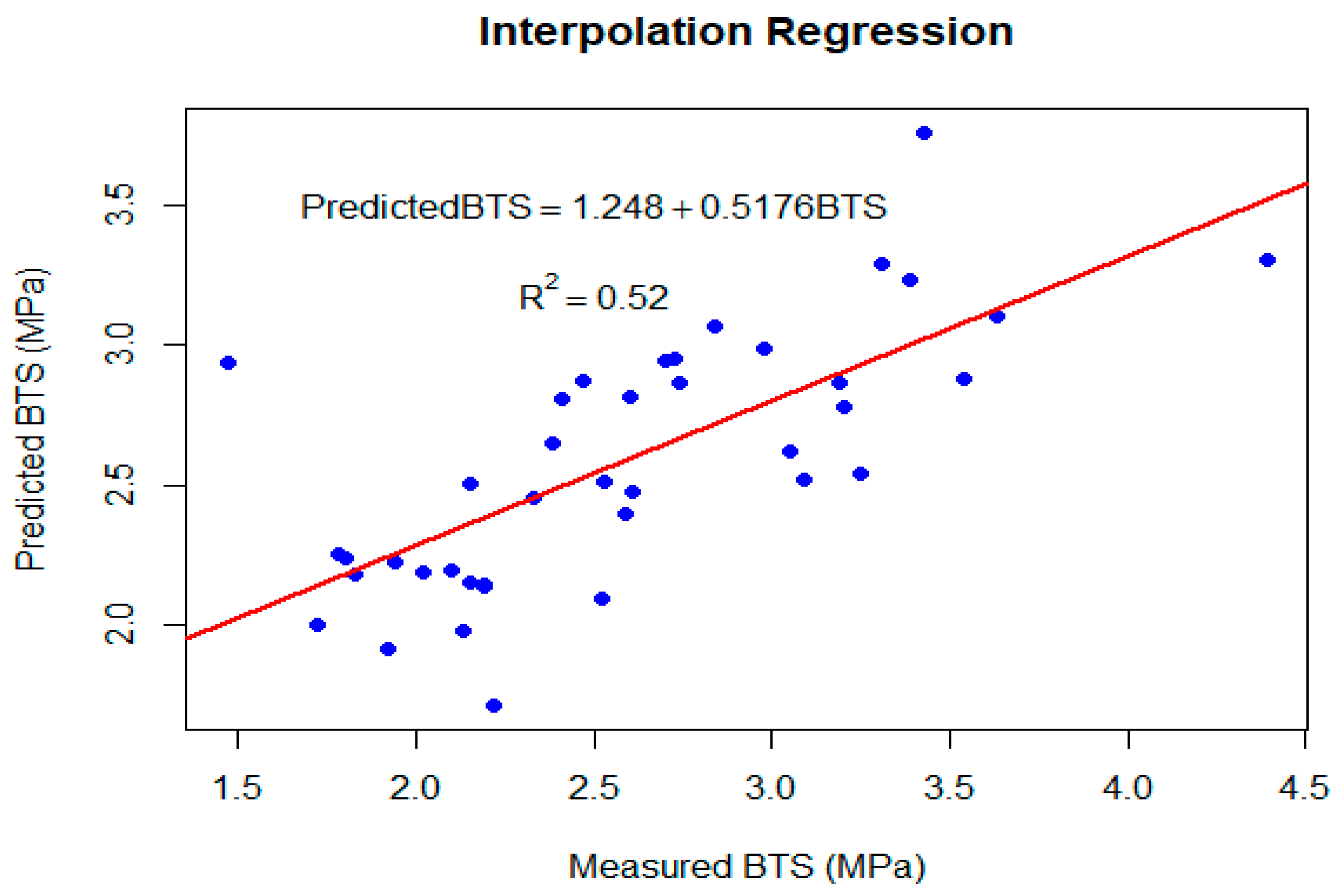
To determine the best regression model for the normalized training set, we used regression feature selection methods such as forward selection, backward elimination, and the best subsets. All these methods unanimously selected the second-order regression model with two explanatory variables, Id2 and Gs. All the parameters were highly significant (see Table 3), and the coefficient of determination R2 and adjusted R2 were 51.8% and 50.5%, respectively. Figure 5 shows the predicted values from the interpolated regression model.
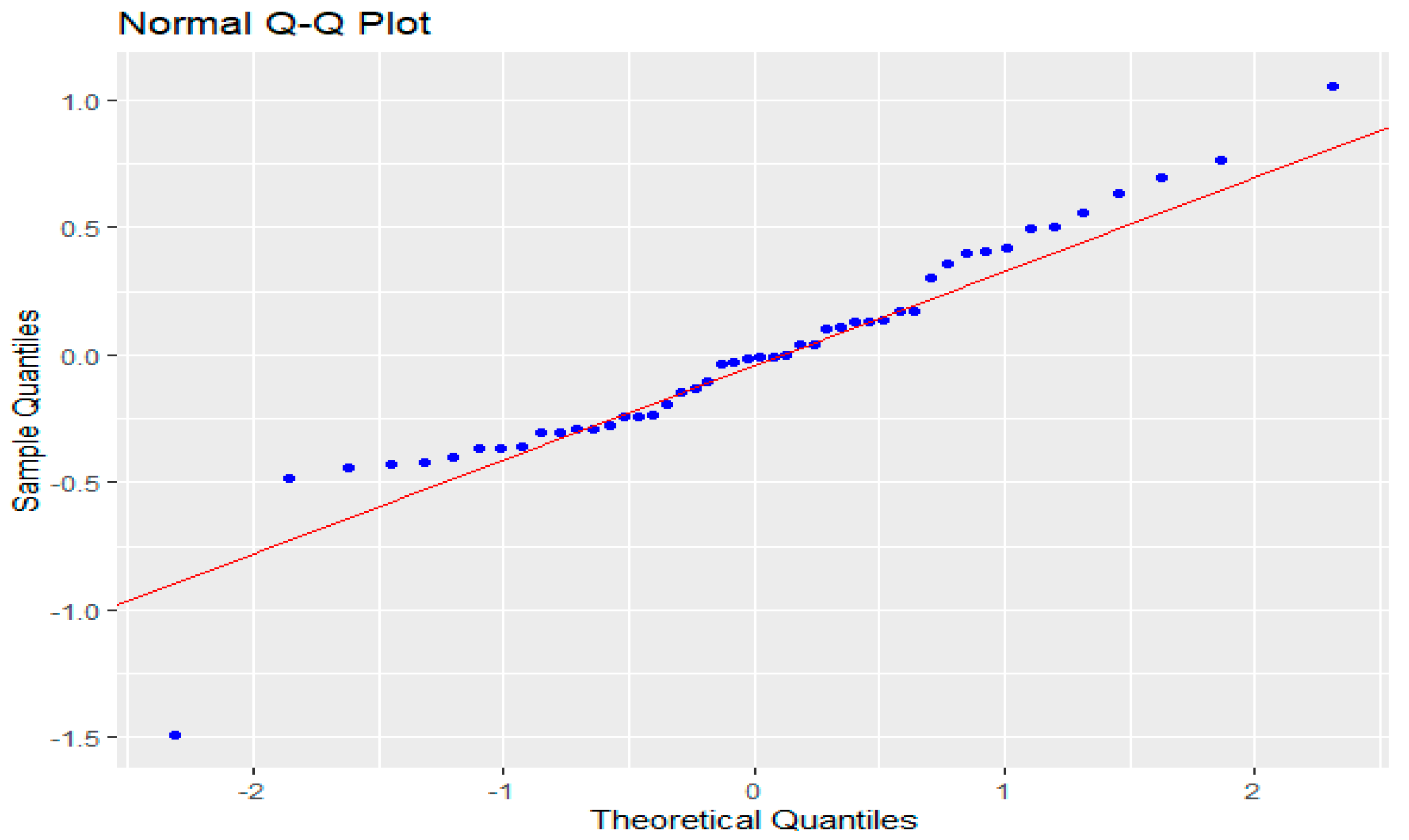
The normality test of the residuals is shown in Figure 6. The p-value of the Kolmogorov–Smirnov test exceeded 15%, which clearly shows that there was no deviation from normality. Besides, the variance inflation factor (VIF) was very low (1.14), indicating that multicollinearity was not detected. VIF values exceeding 10 were regarded as indicative of multicollinearity.
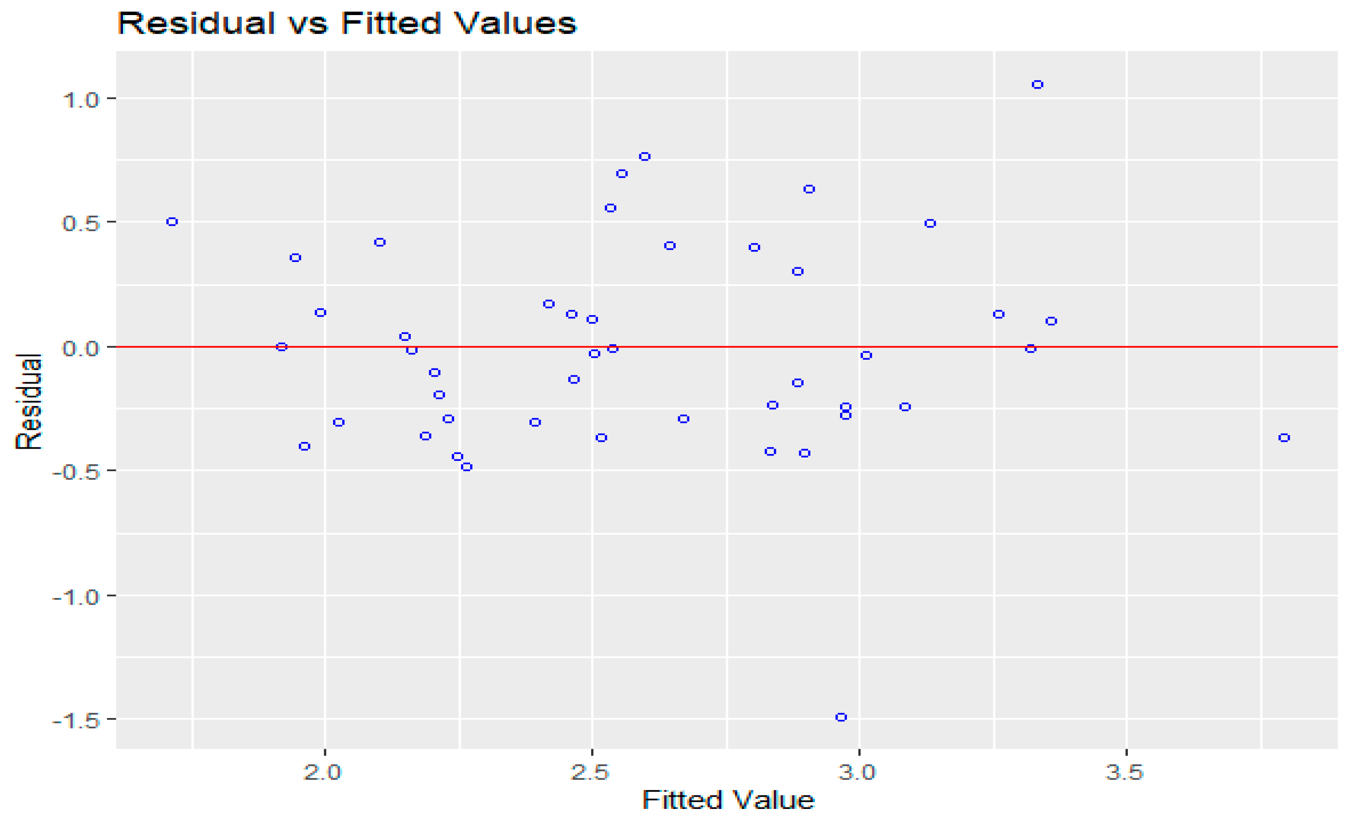
Figure 7 shows a diagnostic plot for the residuals of the model. The residual plot in Figure 7 did not show any pattern of heteroscedasticity in the “nonconstant error variance”. To test the correlation among the residuals, the Durbin–Watson test was performed, and a test statistic of d = 2.50 was obtained. At the 5% significance level, the upper critical value of the test was du, 0.025 = 1.51; clearly, the observed value of the test statistic was larger than both du, 0.025 and 4-du, 0.025, these critical values support the claim that those errors are not correlated.
The family of penalized regression techniques was an alternative to MLR models and examples of these family include Ridge, Lasso, and Elastic Net. Lasso and Elastic Net are feature selection tools as well as predictive modeling techniques. These models apply regularized constraints (λ, α) to the model coefficients and shrink some of them to zero. To determine the optimal regularization parameter λ for these models, the cv.glmnet, and glmnet R packages were used. These functions use penalized maximum likelihood method to fit generalized linear models. The Ridge, Lasso, and the Elastic Net model paths were fitted using the mean-squared error CV criterion. The workflow of the methodology of the study is summarized in Figure 8.
First, a sequence of n lambdas was generated, and the training dataset was divided into K = 10 folds. The model was cross-validated n times using nine subsamples as the training set and the remaining sample as the test set. Each time, as MSE was computed, a fold was removed and a different one was chosen. The lambda value with the smallest MSE was chosen, and the best model was fitted. The upper panels of Figure 9 show CV MSE as a function of log (λ). The vertical dashed lines in these plots represent the log (λ) value with the minimum MSE and the largest value of log (λ) within one standard error to that of log (λ) with the minimum MSE for the Ridge and Lasso models, respectively.
The plots in the lower panels of Figure 9 show the shrinking of the coefficients of the Ridge and Lasso models as a function of log (λ). All the coefficients of the Ridge and Lasso models approach zero at log (λ) = 4 and −1.5, respectively, whereas those of the Elastic Net approach zero at log (λ) = 1. For the Elastic Net, the best value of the regularization parameter estimate is λ = 0.007, corresponding to α = 0.1.
The mean square error of each model was calculated, and the (λ, α) values with the minimum mean square error were chosen to build the best model. The estimates of these parameters for the four competing regression models with their root mean squares (RMSE) are listed in Table 4.
The results of the information criteria for the 10-fold CV for the four regression models are listed in Table 5. These results show no apparent differences among the four regressions models; all the accuracy measurement results are close.
Figure 10 shows the performances of the compared models. The R2 values of the models indicate that the ANNS outperformed all the other models.
The results of the accuracy measurements, i.e., RMSE, MAE, and R2, are listed in Table 6 for comparing the performances of the six models. The R2 and MAE values indicate that the ANNS model outperformed all the other fitted models. With regard to RMSE, the Lasso and MLR models have a slight advantage over the other models. Penalized regression methods work very well when the number of explanatory variables is large, whereas ANNS performs best when the sample size is large.
6. Conclusions
In this study, six methods, namely, ANNS, ANNN, Ridge regression, Lasso regression, MLR, and Elastic Net regression, were examined to build a model that can be used to predict BTS. Most of these methods perform variable selection, which is the process by which a reduced number of independent variables is chosen, as well as prediction. Both ordinary least squares and maximum likelihood methods were used to fit the BTS data to these models. Those are well-known methods that can provide highly accurate predictions. The limitations of those methods were investigated using 10-fold CV criteria, and the results have demonstrated all the methods are useful and competitive for use along with the other existing modeling methods. Another key limitation of this study is the size of the data. However, these samples were the averages of large sample sizes with unequal lengths. Such cases are more common when the cost of the extraction is very high or it is difficult to obtain enough samples. Prediction results from the six best models produced by the above techniques are compared by using Root Mean Square Error (RMSE), Absolute Mean Error (MAE), and the coefficient of determination (R2). Based on the results of the RMSE, the accuracy of the predictions for the BTS values obtained from all the competing models are very close, but the results of the MAE and R2 have shown that the Keras sequential model outperformed the other competing models. Although this dataset indicated the simplicity and the potential superiority of the ANNS model, but ANNS is closely adapted to the training data, and exploiting its broad flexibility demands ingenuity in choosing the estimation method to achieve high accuracy prediction. Besides, Elastic Net and Lasso play an important role in the studies with small sample sizes that have large number of parameters. In such cases, those techniques, which are mainly used for the analysis of small samples, are the best candidates to be employed for the modeling and the prediction of such data types.
Author Contributions
Conceptualization, H.A. and M.Y.H.; methodology, M.Y.H.; software, M.Y.H.; investigation, H.A.; data acquisition, H.A. and M.Y.H.; validation, M.Y.H.; Formal Analysis, M.Y.H.; supervision, writing—original draft, writing—review and editing, H.A. and M.Y.H. All authors have read and agreed to the published version of the manuscript.
Funding
The field and laboratory studies of this study were supported by a grant from the United Arab Emirates University, Research Affairs, under the title of UPAR 2016–31S252 program. The obtained data were used to prepare this paper.
Acknowledgments
The authors would like to thank their research associates, technicians, and students who were involved in various stages of this study.
Conflicts of Interest
The authors declare no conflict of interest.
References
- Baykasoglu, A.; Güllü, H.; Çanakçi, H.; Özbakir, L. Prediction of compressive and tensile strength of limestone via genetic programming. Expert Syst. Appl. 2008, 35, 111–123. [Google Scholar] [CrossRef]
- Arman, H.; Abdelghany, O.; Saima, M.A.; Aldahan, A.; Mahmoud, B.; Hussein, S.; Fowler, A.; AlRashdi, S. Strength estimation of evaporitic rocks using different testing methods. Arab. J. Geosci. 2019, 12, 1–9. [Google Scholar] [CrossRef]
- Hasanipanah, M.; Zhang, W.; Armaghani, D.J.; Rad, H.N. The potential application of a new intelligent based approach in predicting the tensile strength of rock. IEEE Access 2020, 8, 57148–57157. [Google Scholar] [CrossRef]
- Arman, H. Correlation of uniaxial compressive strength with indirect tensile strength (Brazilian) and 2nd cycle of slake durability index for evaporitic rocks. Geotech. Geol. Eng. 2021, 39, 1583–1590. [Google Scholar] [CrossRef]
- Altindag, R.; Guney, A. Predicting the relationships between brittleness and mechanical properties (UCS, TS and SH) of rocks. Sci. Res. Essays 2010, 5, 2107–2118. [Google Scholar]
- Farah, R. Correlations between index properties and unconfined compressive strength of weathered Ocala limestone. Univ. Tech. Rep. Master’s Thesis, University of North Florida, Jacksonville, FL, USA, 2011; p. 142.
- Kahraman, S.; Fener, M.; Kozman, E. Predicting the compressive and tensile strength of rocks from indentation hardness index. J. S. Afr. Inst. Min. Metall. 2012, 112, 331–339. [Google Scholar]
- Nazir, R.; Momeni, E.; Armaghani, D.J.; Amin, M.F.M. Correlation between unconfined compressive strength and indirect tensile strength of limestone rock samples. Electron. J. Geotech. Eng. 2013, 18, 1737–1746. [Google Scholar]
- Kallu, R.; Roghanchi, P. Correlations between direct and indirect strength test methods. Int. J. Min. Sci. Technol. 2015, 25, 355–360. [Google Scholar] [CrossRef]
- ISRM. Suggested Methods, Rock characterization testing and monitoring. In International Society of Rock Mechanics. Commission on Testing Methods; Brown, E.T., Ed.; Pergamon Press: Oxford, UK, 1981; pp. 113–114. [Google Scholar]
- Kilic, A.; Teymen, A. Determination of mechanical properties of rocks using simple methods. Bull. Eng. Geol. Environ. 2008, 67, 237–244. [Google Scholar] [CrossRef]
- Heidari, M.; Khanlari, G.R.; Torabi Kaveh, M.; Kargarian, S. Predicting the uniaxial compressive and tensile strengths of gypsum rock by point load testing. Rock Mech. Rock Eng. 2012, 45, 265–273. [Google Scholar] [CrossRef]
- Arman, H.; Hashem, W.; El Tokhi, M.; Abdelghany, O.; El Saiy, A. Petrographical and geomechanical properties of the Lower Oligocene Limestones from Al Ain city, United Arab Emirates. Arab. J. Sci. Eng. 2014, 39, 261–271. [Google Scholar] [CrossRef]
- Karaman, K.; Kesimal, A.; Ersoy, H. A comparative assessment of indirect methods for estimating the uniaxial compressive and tensile strength of rocks. Arab. J. Geosci. 2015, 8, 2393–2403. [Google Scholar] [CrossRef]
- ASTM D Standards. 3967–08, Standard Test Method for Splitting Tensile Strength of Intact Rock Core Specimens; ASTM International: West Conshohocken, PA, USA, 2008. [Google Scholar]
- Singh, T.N.; Verma, A.K.; Sharma, P.K. A neuro-genetic approach for prediction of time dependent deformational characteristic of rock and its sensitivity analysis. Geotech. Geol. Eng. 2007, 25, 395–407. [Google Scholar] [CrossRef]
- Yilmaz, I.; Yuksek, A.G. An example of artificial neural network (ANN) application for indirect estimation of rock parameters. Rock Mech. Rock Eng. 2008, 41, 781–795. [Google Scholar] [CrossRef]
- Yilmaz, I.; Yuksek, G. Prediction of the strength and elasticity modulus of gypsum using multiple regression, ANN, and ANFIS models. Int. J. Rock Mech. Min. Sci. 2009, 46, 803–810. [Google Scholar] [CrossRef]
- Majdi, A.; Beiki, M. Evolving neural network using a genetic algorithm for predicting the deformation modulus of rock masses. Int. J. Rock Mech. Min. Sci. 2010, 47, 246–253. [Google Scholar] [CrossRef]
- Rajesh Kumar, B.; Vardhan, H.; Govindaraj, M. Prediction of uniaxial compressive strength, tensile strength and porosity of sedimentary rocks using sound level produced during rotary drilling. Rock Mech. Rock Eng. 2011, 44, 613–620. [Google Scholar] [CrossRef]
- Monjezi, M.; Khoshalan, H.A.; Razifard, M. A neuro-genetic network for predicting uniaxial compressive strength of rocks. Geotech. Geol. Eng. 2012, 30, 1053–1062. [Google Scholar] [CrossRef]
- Momeni, E.; Jahed Armaghani, D.; Hajihassani, M.; Mohd Amin, M.F. Prediction of uniaxial compressive strength of rock samples using hybrid particle swarm optimization-based artificial neural networks. Measurement 2015, 60, 50–63. [Google Scholar] [CrossRef]
- Hajihassani, M.; Armaghani, D.J.; Marto, A.; Mohamad, E.T. Ground vibration prediction in quarry blasting through an artificial neural network optimized by imperialist competitive algorithm. Bull. Eng. Geol. Environ. 2015, 74, 873–886. [Google Scholar] [CrossRef]
- Mohamad, E.T.; Jahed Armaghani, D.; Momeni, E.; Alavi Nezhad Khalil Abad, S.V. Prediction of the unconfined compressive strength of soft rocks: A PSO-based ANN approach. Bull. Eng. Geol. Environ. 2015, 74, 745–757. [Google Scholar] [CrossRef]
- Faradonbeh, R.S.; Armaghani, D.J.; Monjezi, M. Development of a new model for predicting fly rock distance in quarry blasting: A genetic programming technique. Bull. Eng. Geol. Environ. 2016, 75, 993–1006. [Google Scholar] [CrossRef]
- Khandelwal, M.; Armaghani, D.J. Prediction of drillability of rocks with strength properties using a hybrid GA-ANN technique. Geotech. Geol. Eng. 2016, 34, 605–620. [Google Scholar] [CrossRef]
- Hasanipanah, M.; Noorian-Bidgoli, M.; Jahed Armaghani, D.; Khamesi, H. Feasibility of PSO-ANN model for predicting surface settlement caused by tunneling. Eng. Comput. 2016, 32, 705–715. [Google Scholar] [CrossRef]
- Gordan, B.; Jahed Armaghani, D.; Hajihassani, M.; Monjezi, M. Prediction of seismic slope stability through combination of particle swarm optimization and neural network. Eng. Comput. 2016, 32, 85–97. [Google Scholar] [CrossRef]
- Hasanipanah, M.; Jahed Armaghani, D.; Bakhshandeh Amnieh, H.; AbdMajid, M.Z.; Tahir, M.M.D. Application of PSO to develop a powerful equation for prediction of fly rock due to blasting. Neural Comput. Appl. 2017, 28, 1043–1050. [Google Scholar] [CrossRef]
- Guha Roy, D.; Singh, T.N. Regression and soft computing models to estimate Young’s modulus of CO2 saturated coals. Measurement 2018, 129, 91–101. [Google Scholar] [CrossRef]
- Bejarbaneh, B.Y.; Bejarbaneh, E.Y.; Amin, M.F.M.; Fahimifar, A.; Armaghani, D.J.; Majid, M.Z. Intelligent modelling of sandstone deformation behavior using fuzzy logic and neural network systems. Bull. Eng. Geol. Environ. 2018, 77, 345–361. [Google Scholar] [CrossRef]
- Armaghani, D.J.; Faradonbeh, R.S.; Rezaei, H.; Rashid, A.S.; Amnieh, H.B. Settlement prediction of the rock-socketed piles through a new technique based on gene expression programming. Neural Comput. Appl. 2018, 29, 1115–1125. [Google Scholar] [CrossRef]
- Alavi Nezhad Khalil Abad, S.V.; Yilmaz, M.; Jahed Armaghani, D.; Tugrul, A. Prediction of the durability of limestone aggregates using computational techniques. Neural Comput. Appl. 2018, 29, 423–433. [Google Scholar] [CrossRef]
- Mohamad, E.T.; Armaghani, D.J.; Momeni, E.; Yazdavar, A.H.; Ebrahimi, M. Rock strength estimation: A PSO-based BP approach. Neural Comput. Appl. 2018, 30, 1635–1646. [Google Scholar] [CrossRef]
- Koopialipoor, M.; Jahed Armaghani, D.; Haghighi, M.; Ghaleini, E.N. A neuro-genetic predictive model to approximate over break induced by drilling and blasting operation in tunnels. Bull. Eng. Geol. Environ. 2019, 78, 981–990. [Google Scholar] [CrossRef]
- Mahdiyar, A.; Armaghani, D.J.; Marto, A.; Nilashi, M.; Ismail, S. Rock tensile strength prediction using empirical and soft computing approaches. Bull. Eng. Geol. Environ. 2019, 78, 4519–4531. [Google Scholar] [CrossRef]
- Saedi, B.; Mohammadi, S.D.; Shahbazi, H. Prediction of uniaxial compressive strength and elastic modulus of migmatites using various modeling techniques. Arab. J. Geosci. 2018, 11, 574. [Google Scholar] [CrossRef]
- Saedi, B.; Mohammadi, S.D.; Shahbazi, H. Application of fuzzy inference system to predict uniaxial compressive strength and elastic modulus of migmatites. Environ. Earth Sci. 2019, 78, 208. [Google Scholar] [CrossRef]
- ASTM. D4644–16, Standard Test Method for Slake Durability of Shales and Other Similar Weak Rocks; ASTM International: West Conshohocken, PA, USA, 2016. [Google Scholar]
- ASTM. C97–2, Standard Test Method for Absorption and Bulk Specific Gravity of Dimension Stone; ASTM International: West Conshohocken, PA, USA, 2002. [Google Scholar]
- Chester, D.L. Why two hidden layers are better than one. In Proceedings of the International Joint Conference on Neural Networks, San Diego, CA, USA, 17-21 June 1990; CRC Press: Boca Raton, FL, USA, 1990; Volume 1, pp. 265–268. [Google Scholar]
- Lippmann, R.P. An introduction to computing with neural nets. IEEE ASSP Mag. 1987, 4–22. [Google Scholar] [CrossRef]
- Bishop, C.M. Neural Networks for Pattern Recognition; Oxford University Press: Oxford, UK, 1995. [Google Scholar]
- Ripley, B.D. Pattern Recognition and Neural Networks; Cambridge University Press: Cambridge, UK, 1996. [Google Scholar]
- Sontag, E.D. Feedback stabilization using two-hidden-layernets. IEEE Trans. Neural Netw. 1992, 3, 981–990. [Google Scholar] [CrossRef] [PubMed]
- Hornik, K.; Stinchcombe, M.; White, H. Multilayer feedforward networks are universal approximators. Neural Netw. 1989, 2, 359–366. [Google Scholar] [CrossRef]
- Hoerl, A.E.; Kennard, R.W. Ridge Regression: Biased Estimation for Nonorthogonal Problems. Technometrics 1970, 12, 55–67. [Google Scholar] [CrossRef]
- Hoerl, A.E.; Kennard, R.W. Ridge Regression: Applications to Nonorthogonal Problems. Technometrics 1970, 12, 69–82. [Google Scholar] [CrossRef]
- Santosa, F.; Symes, W. Linear inversion of band-limited reflection seismograms. SIAM J. Sci. Stat. Comp. 1986, 7, 1307–1330. [Google Scholar] [CrossRef]
- Tibshirani, R. Regression Shrinkage and Selection via the Lasso. J. R. Stat. Soc. B 1996, 58, 267–288. [Google Scholar] [CrossRef]
- Tibshirani, R. The Lasso Method for Variable Selection in the Cox Model. Stat. Med. 1997, 16, 385–395. [Google Scholar] [CrossRef] [Green Version]
- Breiman, L. Better Subset Regression Using the Nonnegative Garrote. Technometrics 1995, 37, 373–384. [Google Scholar] [CrossRef]
- Zou, H.; Hastie, T. Regularization and Variable Selection via the Elastic Net. J. R. Stat. Soc. B 2005, 67, 301–320. [Google Scholar] [CrossRef] [Green Version]
- Hastie, T.; Tibshirani, R.; Friedman, J.H. The Elements of Statistical Learning: Data Mining, Inference, and Prediction; Springer: Berlin/Heidelberg, Germany, 2001. [Google Scholar]
- Swingler, K. Applying Neural Networks: A Practical Guide; Academic Press: New York, NY, USA, 1996. [Google Scholar]
- LeCun, Y.; Bottou, L.; Genevieve, O.; Klaus-Robert, M. Efficient backprop in neural networks: Tricks of the trade. Lect. Notes Comput. Sci. 1998, 1524. [Google Scholar]
- Santurkar, S.; Tsipras, D.; Ilyas, A.; Madry, A. How does batch normalization help optimization? Adv. Neural Inf. Process. Syst. 2018, 31, 2488–2498. [Google Scholar]
- Jayalakshmi, T.; Santhakumaran, A. Statistical normalization and back propagation for classification. Int. J. Comput. Theory Eng. 2011, 3, 89–93. [Google Scholar] [CrossRef]
Figure 1.
Geological map of the study area and sampling location [4].
Figure 1.
Geological map of the study area and sampling location [4].

Figure 2.
Scatterplot and the probability plots of the three variables.

Figure 3.
Probability plot of the BTS.

Figure 4.
MSE and MAE as a function of number of epochs.

Figure 5.
BTS values predicted from interpolation.

Figure 6.
Residuals normality plot.

Figure 7.
Regression residual plots.

Figure 8.
Methodology workflow.

Figure 9.
Ridge and Lasso plots as a function of log (λ).

Figure 10.
BTS predicted values.


Table 1.
Partial data used in the study.
| Id2 (%) | Gs | BTS (MPa) |
|---|---|---|
| 34.9 | 2.18 | 2.59 |
| 19.0 | 2.11 | 1.78 |
| 28.0 | 2.14 | 2.59 |
| 17.0 | 2.10 | 1.80 |
| 54.1 | 2.20 | 2.70 |
| 51.9 | 2.36 | 2.02 |
| 20.3 | 2.09 | 2.09 |
| 44.6 | 2.35 | 1.72 |
| 48.8 | 2.18 | 2.47 |
| 8.4 | 2.16 | 2.22 |
| 35.1 | 2.15 | 3.36 |
| 51.1 | 2.09 | 3.46 |
| 53.5 | 2.13 | 3.39 |
| 20.7 | 2.13 | 1.94 |
| 45.7 | 2.16 | 3.19 |
Table 2.
Descriptive statistics of the BTS.
| Variable | Mean | Median | Range | 95% CI for M |
|---|---|---|---|---|
| BTS (MPa) | 2.5819 | 2.5250 | 2.9200 | (2.40, 2.762) |
| Gs | 2.1619 | 2.1500 | 0.3000 | (2.142, 2.181) |
| Id2 (%) | 36.29 | 42.90 | 52.40 | (31.93, 40.64) |
Table 3.
MLR Parameter Estimates.
| Variable | Coeff. | T-Value | p-Value | VIF |
|---|---|---|---|---|
| Constant | 2.5878 | 36.39 | p < 0.001 | |
| Id2 | 0.4622 | 6.00 | p < 0.001 | 1.14 |
| Gs | 0.3006 | −3.91 | p < 0.001 | 1.14 |
Table 4.
Estimates of regularization parameters.
| Model | RMSE | ||
|---|---|---|---|
| MLR | 0 | 0 | 0.435 |
| Ridge | 0.035 | 1 | 0.434 |
| Lasso | 0.009 | 0 | 0.435 |
| Elastic Net | 0.007 | 0.1 | 0.435 |
Table 5.
Comparison of the regression models.
| Model | R2 | MAE | RMSE |
|---|---|---|---|
| MLR | 0.669 | 0.351 | 0.435 |
| Ridge | 0.670 | 0.348 | 0.434 |
| Lasso | 0.670 | 0.349 | 0.435 |
| Elastic Net | 0.670 | 0.348 | 0.435 |
Table 6.
Performance comparison of the models.
| Model | R2 | MAE | RMSE |
|---|---|---|---|
| ANNS | 0.689 | 0.281 | 0.370 |
| ANNN | 0.623 | 0.300 | 0.388 |
| MLR | 0.674 | 0.288 | 0.364 |
| Ridge | 0.672 | 0.295 | 0.368 |
| Lasso | 0.673 | 0.291 | 0.365 |
| Elastic Net | 0.670 | 0.294 | 0.367 |
Publisher’s Note: MDPI stays neutral with regard to jurisdictional claims in published maps and institutional affiliations. |
© 2021 by the authors. Licensee MDPI, Basel, Switzerland. This article is an open access article distributed under the terms and conditions of the Creative Commons Attribution (CC BY) license (https://creativecommons.org/licenses/by/4.0/).
Share and Cite
MDPI and ACS Style
Hassan, M.Y.; Arman, H. Comparison of Six Machine-Learning Methods for Predicting the Tensile Strength (Brazilian) of Evaporitic Rocks. Appl. Sci. 2021, 11, 5207. https://doi.org/10.3390/app11115207
AMA Style
Hassan MY, Arman H. Comparison of Six Machine-Learning Methods for Predicting the Tensile Strength (Brazilian) of Evaporitic Rocks. Applied Sciences. 2021; 11(11):5207. https://doi.org/10.3390/app11115207
Chicago/Turabian StyleHassan, Mohamed Yusuf, and Hasan Arman. 2021. "Comparison of Six Machine-Learning Methods for Predicting the Tensile Strength (Brazilian) of Evaporitic Rocks" Applied Sciences 11, no. 11: 5207. https://doi.org/10.3390/app11115207
Note that from the first issue of 2016, this journal uses article numbers instead of page numbers. See further details here.