Inter-turn Short Circuit Diagnosis Using New D-Q Synchronous Min–Max Coordinate System and Linear Discriminant Analysis


1
Department of Electrical & Automation, Suncheon Jeil College, Suncheon 57997, Korea
2
Department of Electrical and Semiconductor Engineering, Chonnam National University, Yeosu 59626, Korea
*
Author to whom correspondence should be addressed.
Appl. Sci. 2020, 10(6), 1996; https://doi.org/10.3390/app10061996
Submission received: 3 February 2020
/
Revised: 3 March 2020
/
Accepted: 10 March 2020
/
Published: 14 March 2020
(This article belongs to the Special Issue Machine Fault Diagnostics and Prognostics)
Abstract
:In this paper, a direct-quadrature (D-Q) synchronous min–max coordinate system is proposed (as a new method) for diagnosing the occurrence of inter-turn short circuits (ITSC) of three-phase induction motors, and it was found that this method can linearly diagnose such short circuits using only the maximum value of the d-axis current component from the heavy load to the full load. In the diagnosis of ITSC, a method to perform linear discriminant analysis (LDA) efficiently was applied owing to the difficulty of linear separation under light load conditions. In the aforementioned method, time burden is generated because operations are performed for the entire data and between classes. However, the proposed method is useful even when it is applied to the entire load with only the LDA eigenvector of the minimum light load. This is proved by the graphical evaluation of the interaction between the false acceptance rate (FAR) and false recognition rate (FRR), and the results demonstrate that the proposed method is more efficient than existing LDA application methods.
1. Introduction
Induction motors are used in many industrial sites because of their simple structure, good durability, and low cost. However, when the induction motor breaks down owing to certain reasons, it causes extensive damage to the industry. Therefore, a system for managing the induction motor is needed. The main causes of induction motor failure can be classified into mechanical and electrical failures. Electrical failures include stator failure and mechanical failures include rotor and bearing failures [1].
In [2], the incidence of failures of induction motors was analyzed, and it was revealed that stator failure, rotor failure, and bearing failure account for 46%, 26%, and 11%, respectively. Among these types of failures, stator failure can lead to critical failures, which are the focus of diagnosis [3]. In particular, quick detection of inter-turn short circuit (ITSC) is the main research objective [4,5,6,7].
The diagnosing methods are classified into a sensor-based method and a motor electrical signature analysis (MESA) method.
The sensor-based method is divided into wired and wireless methods, according to the development of information and communications technology (ICT).
Although the wired method involves direct coupling, recent developments in wireless communication technology have enabled diagnosis without direct coupling. Furthermore, many research studies have been conducted based on the aforementioned developments [8,9,10]. Typically, amplitudes of frequencies ratio 50 s frequency coefficient (MSAF-RATIO-50-SFC), MSAF-RATIO-50-SFC-EXPANDED, MSAF-RATIO-24-MULTIEXPANDED-FILTER-8, and the shortened method of frequencies selection (SMoFS-15) are normally used, but the analysis is somewhat complicated [11,12].
Since 1989, FFT has been used for the diagnosis of a stator using MESA [13]. Later, Park’s vector approach (PVA) was studied to diagnose in a rotating state [14,15,16]. PVA transformed three phases into two-phase orthogonal equations to diagnose failures in a rotating state in a circular pattern. However, due to the power factor problem of the induction motor, there is no difference between the degree of distortion of the normal state and the degree of distortion of the ITSC, which makes it difficult to detect the ITSC. To visualize the PVA, EPVA was studied to analyze the PVA in the form of an ellipse by applying the square root; however, it is difficult to detect the ITSC perfectly [17,18,19].
As the previous studies of MESA only considered the size, simplified methods such as the method using the change of phase angle [20], the one representing the distortion index of the circle by the distortion rate [21], and the half-period frequency analysis method were proposed [22]. However, there is difficulty in the direct diagnosis of ITSC.
In addition, the three-phase source of voltage and current of the MESA is used for voltage total harmonic distortion (VTHD) of IEEE Std. 519, current unbalance factor (CUF) of IEC60034-1, voltage total harmonic distortion (VTHD), each voltage harmonic distortion (EVHD), current total harmonic distortion (CTHD), and each current harmonic distortion (ECHD) of IEEE Std. 519 [23,24,25,26].
While such various characteristic diagnostic methods exist, complete diagnosis is difficult even if the diagnosis is performed using the MESA and the sensors. Particularly at light loads, it is difficult to diagnose using these methods. To solve this problem, AI technology can be used.
It was proven that Neural Network (NN) classifier is a good approach in terms of classification speed, accuracy, and suitability for hardware implementation. In the application of this technology, the approach using the motor current signature analysis(MCSA), the sensor, and the complex method was used, and it depends on the sampling and fast fourier transform(FFT) methods, according to the current of each phase and the measured values of the sensors [27].
The PVA method, which was described above, is inefficient because it is difficult to apply; furthermore, it is inefficient owing to the influence of noise, according to [28]. For the direct sampling method, it is difficult to extract samples for a time variation; therefore, samples are artificially extracted. Although the FFT method uses kurtosis, skewness, crest factor, clearance, and shape factor as feature values, steady-state induction motors also exhibit three harmonic characteristics, which add some time burden to the NN [29].
Many papers on artificial intelligence (AI) technology have been reported to classify stator failures, rotor failures, and bearing failures, and studies on changes in speed or load should be conducted.
Meanwhile, in order to minimize the time burden of AI learning and recognition, feature extraction methods such as LDA and PCA have been studied. [30] showed that the LDA method is superior to the stator failure diagnosis method and proved its usefulness. In [29], LDA is used for FFT as a diagnostic method according to the speed change, but in the method of LDA calculation, the LDA should be recalculated for each speed in the entire LDA operation. Furthermore, it causes a time burden on the application and recognition of AI’s learning data. In addition, as many papers depend on FFT to apply LDA, a new method is needed.
In this paper, a new method using the direct-quadrature (D-Q) synchronous min–max coordinate system is proposed for ITSC diagnosis, through which the effective LDA application method is explained. To demonstrate the performance of this method, the interaction between false acceptance rate (FAR) and false recognition rate (FRR) was verified graphically. This is a method for determining whether linear separation is well performed through the relational analysis of FAR and FRR; the effectiveness of this method can be proved when it is applied to future AI diagnosis technologies [31,32].
The organization of this paper is as follows. The turn short, D-Q transformation, and min–max coordinate system are defined in Section 2, LDA is described in Section 3, and the FAR-FRR interaction graph is described in Section 4 to demonstrate the efficiency. Finally, experiments and results are discussed in Section 5.
2. Turn Short and D-Q Transformation
2.1. Stator Failure
In Figure 1, the short circuit in phase A indicates an event where a short circuit occurs in a turn that is distant from the first turn, and in the case of phase B, the short circuit between coils is shown. In the case of phase C, a minute short circuit in which the adjacent turns (first and second turns) are shorted is shown.
As such, a short circuit that may occur in the stator can cause a short circuit between coils and a short circuit between turns. When this fault occurs, induction motors are subject to severe vibrations and heat generation.
However, it is difficult to diagnose a fine turn short circuit because no significant difference is observed between the steady state and the pulsation due to losses such as iron loss and copper loss of the induction motor. Nevertheless, when ITSC occurs, it is necessary to detect ITSC because local heating and breakdown conduction cause a serious failure.
On the other hand, although a three-phase induction motor should be able to diagnose in the on-line state of rotation, the analysis is difficult in the time-varying state. Therefore, the D-Q transformation method is converted from three-phase to two-phase for easier analysis.
2.2. D-Q Transformaion
Computation is complex for direct control of three-phase voltage currents, and it is difficult to apply control algorithms. Therefore, the D-Q transformation technique is commonly used for accessing three-phase voltage and current as a direct current voltage. Although in this D-Q transformation, when the ideal three-phase power is supplied, the peak value of the phase voltage and zero are produced as outputs, actual phase power includes noise and harmonics, and phase unbalance exists. The D-Q transformation is divided into a static coordinate system, which converts three-phase current or voltage into two-phase current or voltage as shown in Figure 2a and a synchronous coordinate system, which rotates the stationary coordinate system according to angular speed to produce a DC output as shown in Figure 2b.
These can be expressed in equations as follows.
where is the current in phase a, is the current in phase b, is the current in phase c, is the d-axis current by D-Q transformation, and is the current in phase q, which is called the static coordinate system. If the three phases are in parallel, .
At this time, to find the position of the rotor, or the reference magnetic flux θ and match the magnetic flux component to it, it must be rotated about the origin by θ, and this can be calculated using Equation (2).
and , which are obtained by Equation (2), are called d-q synchronous coordinate systems. Ideally, will show a DC component, and will always produce zero.
The output waveforms obtained through this process are shown in Figure 3.
Figure 3 shows the change in the current owing to D-Q transformation. Figure 3a shows a three-phase input current, Figure 3b shows a D-Q stationary coordinate system from three-phase to two-phase, and Figure 3c shows a D-Q synchronous coordinate system. As shown in Figure 3c, the synchronous coordinate system can be expressed by DC components when it is ideal.
However, the actual waveforms are irregular and have periodic pulses instead of producing outputs with DC components due to noise and harmonics.
2.3. D-Q Transformation Analysis According to Turn Short
When turn short circuits occurs in one phase as shown in Figure 4a, an independent closed circuit is created through , and as shown in Figure 4b, the independent closed loop is also created during D-Q transformation. If the number of turns with the short circuit is , the number of turns with no short circuit is , the total number of turns is , .
Shorted and unshorted windings have the same inductance, resulting in direct interference.
This interference generates an induced electromotive force in the shorted windings when it is present in inductances with the same magnetic flux, and this induced electromotive force generates a short circuit current, . When a turn short occurs, is large; therefore, the induced electromotive force becomes large. As the short-circuit resistance becomes small, the short-circuit current becomes large.
As shown in Figure 5a, two inductances exist in the inductance on one phase due to the occurrence of , as shown in Figure 5b. Between two inductances, the magnetic flux is interlinked with each other.
In this case, if the inductance on one phase according to the number of turns is and the inductance by a short circuit is , the interlinked magnetic flux can be defined as Equations (3) and (4).
where is the interlinked magnetic flux in one phase, is the interlinked magnetic flux of a fault inductance generated at the turn short circuit, is the flux in one phase, is the magnetic flux of a fault inductance, and is the steady current in one phase.
When a turn short occurs, the two magnetic fluxes behave like a transformer, and the two interlinked magnetic fluxes generate leakage flux. Accordingly, the sum of the magnetic flux leakage by a short circuit, , is given by Equation (5).
In Equation (5), the total flux decreases as a result of . The generated short circuit current becomes , and the total magnetic flux is further reduced. If is term A, is term B, is the case when the first short circuit occurs, and is negligible because it is small for a negligible turn short circuit, then the variation of current can be confirmed by the relational analysis of . In this case, it can be found that in term B is reduced by compared to in term A. Furthermore, it can be found that the total magnetic flux becomes smaller when the first short circuit occurs.
On the other hand, if the case where the short circuit becomes significant is . As increases, the value of becomes smaller than that of . In other words, when the short circuit becomes significant, term B becomes smaller, and the change in the magnetic flux increases than when the first short circuit occurs.
It can also be found from the cyclic solenoid equation in Equation (6) that the relationship between the inductance L and the number of turns N is not linear.
where is the conductor dielectric constant, is the cross-sectional area of the stator core, and is the average length of the coil. From a cyclic solenoid’s perspective, it has a relationship of , and thus when occurs, changes as . The difference in the decrease in term A from B is insignificant.
In other words, it can be found that when the short circuit occurs, the total magnetic flux decreases, but as the short circuit becomes significant, the magnetic flux increases again.
However, ITSC shows a different case.
In Equation (5), is very small; thus, the value of can be assumed to be 1. In the case of , it can also be ignored by insulation resistance; thus, the result of the steady-state interlinked magnetic flux is obtained and only the inductance component is changed by a minute short circuit. Therefore, and can be obtained from Equation (7).
The schematic is shown in Figure 6.
In Figure 6, the x-axis and y-axis represent the increasing turn short circuits and magnitude of the current, respectively. The ITSC is a minute turn short circuit, which implies that only two windings are shorted for the total number of turns, and the four-turn, six-turn, eight-turn, and twelve-turn short circuits are the cases when four, six, eight, and 12 windings are shorted, respectively. It is classified into classes as shown in Figure 6.
However, in general, the current of the DC component pulsates due to the efficiency of the motor, and the amplitude becomes larger when the turn short is increased. In this study, the D-Q min–max coordinate system was applied to the diagnosis of ITSC by considering the maximum and minimum values of the amplitude in order to apply the D-Q synchronous coordinate system.
3. LDA
Although the method presented in Section 2 can be applied to heavy and maximum loads, it is difficult to apply it directly to light loads with a small change. Therefore, it is necessary to apply AI to linearly separate it and to align feature patterns so that AI technology can be efficiently applied.
In general, the reason why LDA shows excellent performance by feature extraction is that the patterns in normal and fault condition are similar, and therefore, those can be applied to AI technology. LDA maps the dimension based on the main axis that maximizes class separation in the feature space to keep the classification information between classes in a maximum way by maximizing the ratio between between-class scatter (BCS) and within-class scatter (WCS).
First, the measured data are converted into column vectors, and then , which is a BCS matrix, and , which is a WCS matrix, are obtained by Equations (8) and (9).
where represents the number of data in the i-th class, , and represents the average value in the i-th class, . In Equation (8), m is an average value of all classes.
Equations (8) and (9) are used to calculate the Γ values in Equation (10) in the i-th frequency component, and then the frequency components are selected in the order of the higher ratio values. In other words, the value of Γ indicates that the BCS value is large and the WCS value is small. Therefore, it is a method of extracting the difference in the order of the fault by using Γ value.
On the other hand, many papers have obtained the data of normal operation and failure for each type of failure (stator failure, rotor failure, and bearing failure), and even if LDA is applied to the entire data, excellent results were obtained for AI technology.
However, the BCS of the total LDA, the WCS for each speed, and the BCS and WCS for the total change must also be considered to meet Equation (9). Therefore, the timing burden occurs to overall computation time.
The objective of this paper is to reduce the time burden on learning and diagnosis of AI diagnosis technology in the same failure. The failure characteristics of the D-Q synchronous coordinate system from light loads to full loads were analyzed by applying LDA, and an efficient LDA application method was proposed.
4. FAR–FRR Interaction Graph
FAR, which is generally used in biometrics, refers to a case where a fault state is recognized as a normal state, and FRR indicates a case where a false state is recognized as a fault state.
Figure 7 illustrates the FAR–FRR interaction graph.
In Figure 7, it can be found that FAR and FRR are independent and inversely proportional to each other. The lower the FAR, the higher the corresponding FRR. Conversely, the lower the FAR, the higher the FAR. In other words, FAR and FRR are inversely related, not interdependent. Higher FAR implies that the normal state is recognized as a failure state because the FRR is reduced, while higher FRR implies that the FAR is lowered to recognize the failure as normal, and this should be close to 0 for high performance. In this regard, the point where FAR and FRR become identical is used as a threshold, and this is called an equal error rate (ERR).
The reason for evaluating based on this recognition method is that AI technology can improve the performance and reduce computation time depending on how well the normal and fault data are separated. Furthermore, the separation between the two data can be confirmed without applying AI.
5. Experiment and Discussion
5.1. Experimental Conditions
In this experiment, a 3-phase induction motor with the specifications as in Table 1 was used.
In addition, the experiment was performed under the following conditions to consider changes in the load conditions.
- Operation of an induction motor by using inverter;
- Adjustment of the motor operation speed by using dynamometer;
- The initial speed—the rated speed 1690 (rpm);
- Operating time—turn short per 30 (s);
- Sampling rate and the number of samplings: 10,000 (S/s), 10,000 (s).
The current was measured using an i5s AC current clamp by Fluke, and data were collected using a USB-DAQ 9215A with BNC by National Instruments.
Figure 8 shows the structure of the total system.
The measurement result of the input stage showed that the input power contained noise, as shown in Figure 9a. Thus, the cut-off frequency was set at 100 Hz by Butterworth third-order IIR filtering, and the filtering was processed as shown in Figure 9b.
Furthermore, the short of the stator winding was configured artificially as shown in Figure 10a, and the winding was connected to an external tab as shown in Figure 10b.
Table 2 shows a turn-to-turn short circuit according to the tab connection. It shows the ITSC when turns no. 1–3 were connected. When turn no. 5 was connected, the turn-to-turn short circuit increased to a 4-turn short.
5.2. D-Q Synchronous Min–Max Coordinate System
The reason why the diagnosis of ITSC using the PVA method is difficult is that the maximum and minimum values based on the vector scalar sum of the d-axis and the q-axis are expressed as ratios. This is based on the pulsation of the current based on the interlinked magnetic flux analysis described above.
In this paper, a change in the magnitude of the short-circuit current is generated for linear diagnosis of ITSC. To apply it to the experiment, the D-Q synchronous min–max coordinate system over time was proposed.
Figure 11 shows the results of monitoring the steady-state (black line), ITSC (red line), 4-turn short circuit (green line) and 6-turn short circuit (blue line) under full load using the proposed D-Q synchronous coordinate system. As shown in Figure 11, the induction motor in steady state contains irregular AC component pulsating due to a loss. It can be found that the amplitude in the ITSC state is not significantly different from that in the steady state. However, it can be found that the overall value of the current increases, and from the 4-turn short circuit, the amplitude becomes larger.
Figure 12 shows the results of monitoring the no-load condition using the D-Q synchronous coordinate system. As shown in Figure 12, a short circuit over 4-turn can be diagnosed as the characteristic point as the amplitude becomes larger. In the case of ITSC, however, the pulse width is similar to that in the normal state, making diagnosis difficult.
Figure 13 shows the maximum and minimum values of AC components pulsating from no load to full load by extracting 90 samples per second in the min–max coordinate system.
In the 1690 rpm region in Figure 13, the results described in Figure 6 can be observed. Through this, it can be found that linear separation is possible through the max value of id and the min–max coordinate system in the region up to heavy load or full load and that the ITSC can also be linearly separated. However, under no-load and light load conditions, more than 6-turn short circuits may be linearly separated, but it is difficult to separate ITSC and 4-turn short circuits. Therefore, they will need diagnostic techniques combined with AI technology.
5.3. Efficient LDA Application Method
In the existing papers, the method of applying LDA is used to obtain the entire data and to project it with the eigenvector through LDA and to align it with AI technology. Even in the general short-circuit situation of the stator, excellent performance can be observed.
If LDA is applied to D-Q synchronous min–max coordinate system, which was proposed in this paper, as shown in Figure 13, eigenvector w = [−0.704105, 0.710096] can be obtained as shown in Figure 14, and an optimal rotation direction of LDA was −45.243° to obtain optimal direction information. In this case, since the general turn short was assumed, the ITSC was excluded.
In Figure 14, the red dotted line shows the eigenvector w line obtained by LDA, and the red solid line shows the optimal critical line when the rotation angle is transformed according to the eigenvector. As shown in Figure 14, a general turn short circuit enables stable diagnosis even at a light load.
However, if LDA is used to diagnose ITSC, it can be found from Figure 15 that diagnosis is difficult not only at light load but also at full load.
In Figure 15, the blue solid line indicates the critical line when only the max value of is used at full load, the blue box on the upper right indicates the class of full load at 1690 rpm, black dots indicate the steady state, the red dots in the blue box on the upper right indicate the ITSC, and the red dots overlapping the class of the black dots indicates the ITSC class at 1700 rpm. As shown in Figure 15, it can be effectively applied to LDA at light load. Under full load, however, it can be found that the separation is not efficient compared to the method using the max value of Id, and the existing LDA application method is not efficient.
5.4. Light Load LDA Application Methods
The definition of the light load condition is required for efficient analysis at light loads. Generally, light loads are defined as light loads, but it is difficult to define exact numerical situations.
However, in this paper, the light load condition is defined based on the difference of BCS change. The result of analyzing the BCS difference between each class in the steady state and the ITSC state is shown in Figure 16.
In other words, a range between 1790 rpm and 1750 rpm can be defined as a light load, beyond which loads can be defined as heavy load and full load.
On the other hand, under light load conditions, the BCS is very smooth and shows no significant difference.
In general, for heavy LDA application, it is time-consuming to calculate LDA for the entire load and then LDA for each class. However, the BCS analysis shows that there is no significant change at light load. We believe that this can be effectively applied to all light loads with only one condition of light loads without having to calculate each class. For example, even if the LDA eigenvector for 1790 rpm is applied to calculate LDA for 1760 rpm, an accurate diagnosis is possible and thus it is not necessary to perform a class analysis for 1760 rpm.
In order to prove this, the interaction graph of false acceptance rate (FAR) and false rejection rate (FRR), which are used as the identification tool of bio-recognition, is shown.
To demonstrate the efficient method at light load, eigenvector w = [−0.704105, 0.710096] for 1790 rpm can be obtained. −15.022° of rotation direction by LDA is obtained as optimal direction information. Table 3 shows the LDA direction information for each speed.
Figure 17 is a FAR–FRR graph that compares the normal class and the ITSC class that were measured at 1790 rpm.
In Figure 17, the black line is the result of analyzing FAR–FRR without changing the angle, the red line is the result of applying an angle of −15.022°, and the green line is the result of applying an angle of −45.243°, which is the angle from 1790 rpm to 1690 rpm, to the class for 1790 rpm. This shows that when the LDA was calculated from the entire data to be applied to a specific class (green), the performance was lower than when each class was analyzed (red).
The FAR–FRR interaction graph is shown in Figure 18.
In Figure 18, the black line indicates the result without an angle conversion, the red line indicates the result when only the LDA of 1790 rpm class was applied, and the green line indicates the result when the LDA of 1790–1690 rpm was applied to the angle at 1790 rpm.
As shown in Figure 18, it is better to apply to one class than to the class in the whole data, and the performance is slightly better compared to the case without the angle conversion.
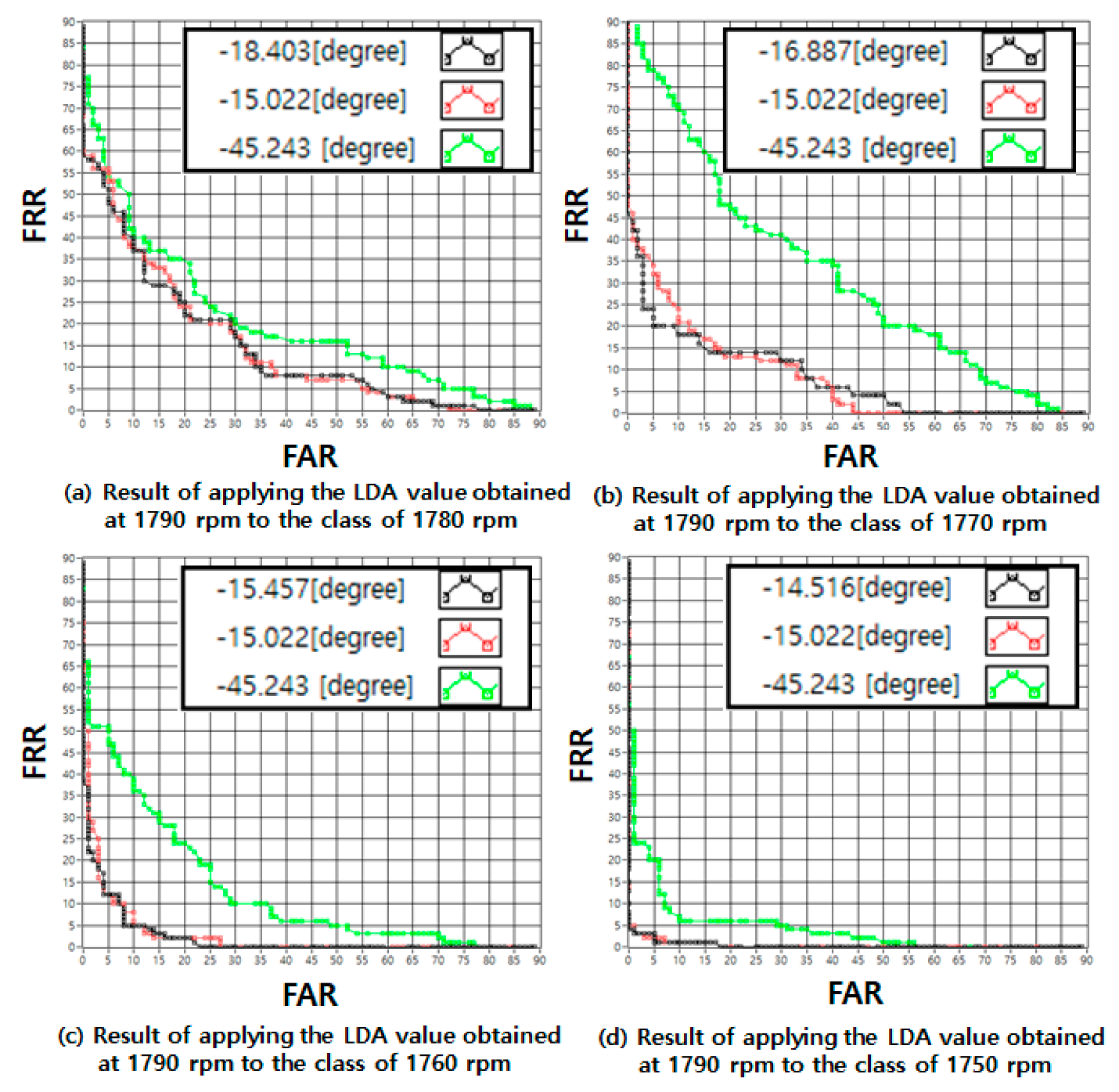
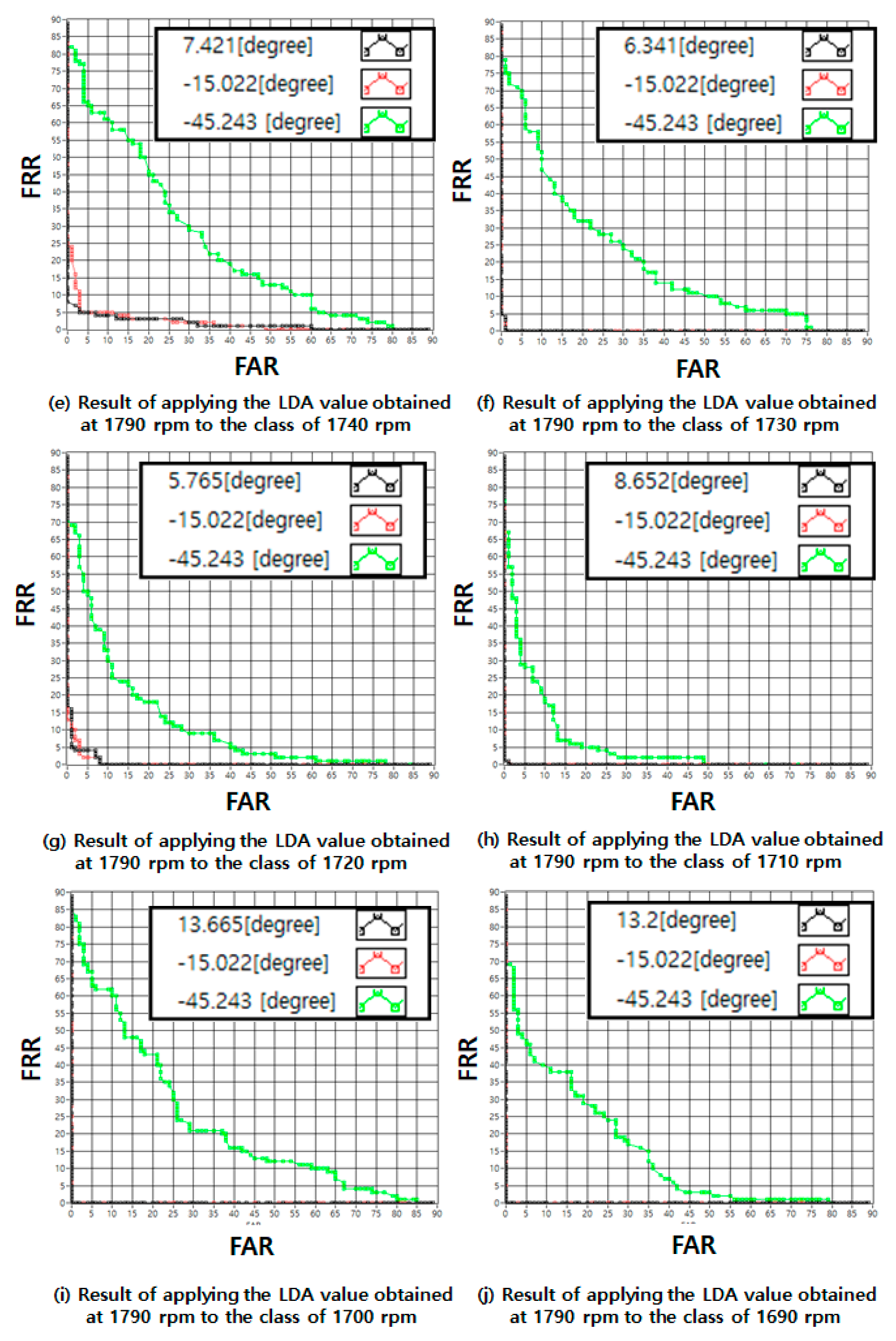
Figure 19 shows the result of the FAR–FRR interaction graph when only −15.022° at the minimum light load speed of 1790 rpm was applied to each speed class.
Figure 19a shows the result of applying the LDA degree value obtained at 1790 rpm to the class of 1780 rpm, and Figure 19j shows the result of applying the class to 1690 rpm. Here, the black line is the result of applying LDA degree by each class (e.g., in Figure 19a, black line is FAR–FRR interaction graph by LDA degree of 1780 rpm), the red line is the result of applying LDA degree of 1790 rpm, and the green line is the result of applying the LDA degree value of 1790–1690 rpm to the class of the corresponding speed.
As shown in Figure 19, even if the LDA is not recalculated for each class, the LDA value of the minimum light load speed shows good performance or similar performance at all speeds. In general, the separation performance is better than the applied method (green line).
Furthermore, starting from 1730 rpm, it can be found that the black line and the red line are approaching zero, which means that they are linearly separated.
Therefore, in order to apply AI technology for ITSC diagnosis using the DQ synchronous min–max coordinate system, if only LDA of minimum light load speed is obtained and applied to each speed, instead of the conventional LDA technique, it is expected to reduce the burden.
6. Conclusions
In this paper, a new D-Q synchronous min–max coordinate system and an efficient LDA application method for stator ITSC diagnosis were proposed. Using the proposed D-Q min–max coordinate system, it was found that linear separation can be conducted in ITSC diagnosis up to heavy load and full load.
The existing LDA application methods are classified into two methods: a method using the eigenvectors of the entire class and a method obtaining the eigenvectors of the entire class by computing each class.
When operating the first LDA application method, the eigenvector shows that the D-Q min–max coordinate transformation is −45.243°, which is efficient not only at light load but also at full load. This is because ITSC only considering the change of self-inductance as the interlinked magnetic flux is insignificant. As a result, although the variance of the whole class has the eigenvector directionality of LDA, the efficiency is low due to dispersion characteristics that are different from typical turn short circuits.
If the second LDA method is used, the best LDA eigenvectors can be obtained for each class but it causes operation time burden since each class must be operated. Therefore, in order to reduce the computation time for LDA, when the LDA of the minimum light load was applied to the entire speed change (or load change), it was found that the results are similar to those of the existing method. Therefore, providing initial LDA data can be an efficient LDA method for the entire diagnosis.
Recently, a method of pursuing safety with AI diagnostic technology has been proposed, and the proposed method will enable an efficient operation of AI technology.
Author Contributions
Conceptualization, Y.-J.G.; data curation, K.-M.K.; formal analysis, Y.-J.G.; funding acquisition, K.-M.K.; investigation, K.-M.K.; methodology, Y.-J.G.; project administration, K.-M.K.; resources, K.-M.K.; software, Y.-J.G.; supervision, K.-M.K.; validation, K.-M.K.; visualization, K.-M.K.; writing—Original draft, Y.-J.G.; writing—Review & editing, K.-M.K. All authors have read and agreed to the published version of the manuscript.
Funding
This research was respectfully supported by the Technology development Program of MSS [S2666839] and the Ministry of Trade, Industry & Energy (MOTIE) [P036700022].
Conflicts of Interest
The authors declare no conflict of interest.
References
- Waide, P.; Brunner, C. Energy-Efficiency Policy Opportunities for Electric Motor-Driven Systems; IEA Energy Papers; OECD Publishing: Paris, France, 2011; pp. 1–132. [Google Scholar] [CrossRef]
- O’Donnell, P. Report of large motor reliability survey of industrial and commercial installations: Part I and II. IEEE Trans. Appl. 1985, IA-21, 853–872. [Google Scholar] [CrossRef]
- Radja, N.; Rachek, M.; Larbi, S.N. Non-Destructive Testing for Winding Insulation Diagnosis Using Inter-Turn Transient Voltage Signature Analysis. Machines 2018, 6, 21. [Google Scholar] [CrossRef] [Green Version]
- Wang, L.; Li, Y.; Li, J. Diagnosis of Inter-Turn Short Circuit of Synchronous Generator Rotor Winding Based on Volterra Kernel Identification. Energies 2018, 11, 2524. [Google Scholar] [CrossRef] [Green Version]
- Dybkowski, M.; Bednarz, S. Modified Rotor Flux Estimators for Stator-Fault-Tolerant Vector Controlled Induction Motor Drives. Energies 2019, 12, 3232. [Google Scholar] [CrossRef] [Green Version]
- Chen, Y.; Zhao, X.; Yang, Y.; Shi, Y. Online Diagnosis of Inter-turn Short Circuit for Dual-Redundancy Permanent Magnet Synchronous Motor Based on Reactive Power Difference. Energies 2019, 12, 510. [Google Scholar] [CrossRef] [Green Version]
- Goh, Y.J.; Kim, O. Linear Method for Diagnosis of Inter-Turn Short Circuits in 3-Phase Induction Motors. Appl. Sci. 2019, 9, 4822. [Google Scholar] [CrossRef] [Green Version]
- Glowacz, A. Recognition of acoustic signals of induction motor using FFT, SMOFS-10 and LSVM. Eksploat. I Niezawodn. 2015, 17, 569–574. [Google Scholar] [CrossRef]
- Duan, Z.; Wu, T.; Guo, S.; Shao, T.; Malekian, R.; Li, Z. Development and trend of condition monitoring and fault diagnosis of multi-sensors information fusion for rolling bearings: A review. Int. J. Adv. Manuf. Technol. 2018, 96, 803. [Google Scholar] [CrossRef] [Green Version]
- Stief, A.; Ottewill, J.R.; Baranowski, J.; Orkisz, M. A PCA and Two-Stage Bayesian Sensor Fusion Approach for Diagnosing Electrical and Mechanical Faults in Induction Motors. IEEE Trans. Ind. Electron. 2019, 66, 9510–9520. [Google Scholar] [CrossRef] [Green Version]
- Glowacz, A.; Głowacz, Z. Recognition of rotor damages in a DC motor using acoustic signals. Bull. Pol. Acad. Sci. Tech. Sci. 2017, 65, 187–194. [Google Scholar] [CrossRef] [Green Version]
- Glowacz, A.; Glowacz, W. Vibration-Based Fault Diagnosis of Commutator Motor. Shock Vib. 2018, 2018, 10. [Google Scholar] [CrossRef]
- Thomson, W.T.; McRae, C.J. On-Line Current Monitoring to Detect Inter-Turn Stator Winding Faults in Induction Motors. In Proceedings of the 24th Universities Power Engineering Conference, Belfast, UK, 19–20 September 1989. [Google Scholar]
- Cardoso, A.J.M.; Cruz, S.M.A.; Fonseca, D.S.B. Inter-Turn Stator Winding Fault Diagnosis in Three-Phase Induction motors, by Park’s Vector Approach. IEEE Trans. Energy Convers. 1999, 14, 595–598. [Google Scholar] [CrossRef]
- Cruz, S.M.A.; Cardoso, A.J.M. Stator winding fault diagnosis in three-phase synchronous and asynchronous motors, by the extended Park’s vector approach. IEEE Trans. Ind. Appl. 2001, 37, 1227–1233. [Google Scholar] [CrossRef]
- Jung, J.H.; Lee, J.J.; Kwon, B.H. Online Diagnosis of Induction Motors Using MCSA. IEEE Trans. Ind. Electron. 2006, 53, 1842–1852. [Google Scholar] [CrossRef]
- Cruz, S.M.A.; Cardoso, A.J.M. Rotor cage fault diagnosis in three-phase induction motors by Extended Park’s Vector Approach. Electr. Mach. Power Syst. 2000, 28, 289–299. [Google Scholar] [CrossRef]
- Parra, A.P.; Enciso, M.C.A.; Ochoa, J.O.; Peñaranda, J.A.P. Stator fault diagnosis on squirrel cage induction motors by ESA and EPVA. In Proceedings of the 2013 Workshop on Power Electronics and Power Quality Applications (PEPQA), Bogota, CO, USA, 6–7 July 2013; pp. 1–6. [Google Scholar] [CrossRef]
- Skowron, M.; Wolkiewicz, M.; Kowalska, T.O.; Kowalski, C.T. Application of Self-Organizing Neural Networks to Electrical Fault Classification in Induction Motors. Appl. Sci. 2019, 9, 616. [Google Scholar] [CrossRef] [Green Version]
- Go, Y.J.; Lee, B.; Song, M.H.; Kim, K.M. A Stator Fault Diagnosis of an Induction Motor based on the Phase Angle of Park’s Vector Approach. J. Inst. Control Robot. Syst. 2014, 20, 408–413. [Google Scholar] [CrossRef] [Green Version]
- Yang, C.O.; Park, G.N.; Song, M.H. Study on distortion ratio calculation of park’s vector pattern for diagnosis of stator winding fault of induction motor. Trans. Korean Inst. Electr. Eng. 2012, 61, 643–649. [Google Scholar] [CrossRef]
- Go, Y.J.; Song, M.H.; Kim, J.Y.; Choi, W.R.; Lee, B.; Kim, K.M. A New Algorithm for Analyzing Method of Electrical Faults of Three-Phase Induction Motors Using Duty Ratios Half-Period Frequencies According to Phase Angle Changes. Mechatronics and Robotics Engineering for Advanced and Intelligent Manufacturing. In Lecture Notes in Mechanical Engineering; Zhang, D., Wei, B., Eds.; Springer International Publishing: Cham, Switzerland, 2017; Volume 36, pp. 303–317. [Google Scholar]
- IEC 60034-1. Rotating Electrical Machines—Part 1: Rating and Performance; IEC: Geneva, Switzerland, 2010. [Google Scholar]
- ANSI/IEEE Std. IEEE Recommended Practice for Electric Power Distribution for Industrial Plants; ANSI/IEEE Std.: New York, NY, USA, 1993. [Google Scholar]
- IEEE Std. 519. IEEE Recommended Practices and Requirements for Harmonic Control in Electrical Power Systems; IEEE Std.: New York, NY, USA, 1992. [Google Scholar]
- Chang, H.C.; Jheng, Y.M.; Kuo, C.C.; Hsueh, Y.M. Induction Motors Condition Monitoring System with Fault Diagnosis Using a Hybrid Approach. Engergies 2019, 12, 1471. [Google Scholar] [CrossRef] [Green Version]
- Juan, G.B.; Juan, R.C.; José, R.M.; Pilar, G.G.; Hayde, P.B.; Vicente, A.A. An Approach on MCSA-Based Fault Detection Using Independent Component Analysis and Neural Networks. IEEE Tran. Inst. Measurement 2019, 68, 1353–1361. [Google Scholar] [CrossRef]
- Jeon, B.S.; Lee, D.J.; Lee, S.H.; Ryu, J.W.; Chun, M.G. Fault Diagnosis of Induction Motor by Fusion Algorithm based on PCA and LDA. J. Korean Inst. Iiium. Electr. Install. Eng. 2005, 19, 152–159. [Google Scholar] [CrossRef]
- Mbo’o, C.P.; Hameyer, K. Fault Diagnosis of Bearing Damage by Means of the Linear Discriminant Analysis of Stator Current Features from the Frequency Selection. IEEE Trans. Ind. Appl. 2016, 52, 3861–3868. [Google Scholar] [CrossRef]
- Frosini, L.; Zanazzo, S.; Beccarisi, F. Linear Discriminant Analysis for an Automatic Detection of Stator Faults in Induction Motor Drives. In Proceedings of the 11th International Symposium on Diagnostics for Electrical Machines, Power Electronics and Drives (SDEMPED), Tinos, Greece, 29 August–1 September 2017; pp. 503–509. [Google Scholar] [CrossRef]
- Kim, K.M.; Park, J.J.; Lee, B.; Go, Y.J.; Jung, S.W. Efficient 1:N Fingerprint Matching Algorithm using Matching Score Distribution. J. Inst. Control Robot. Syst. 2012, 18, 208–217. [Google Scholar] [CrossRef]
- Goh, Y.J.; Kim, K.M. A New Matching Score and Threshold Setting Method using Data Mining of Existing Fingerprint Matching Scores Distribution. J. Korean Inst. Intell. Syst. 2019, 29, 170–175. [Google Scholar] [CrossRef]
Figure 1.
Short circuit in slots.
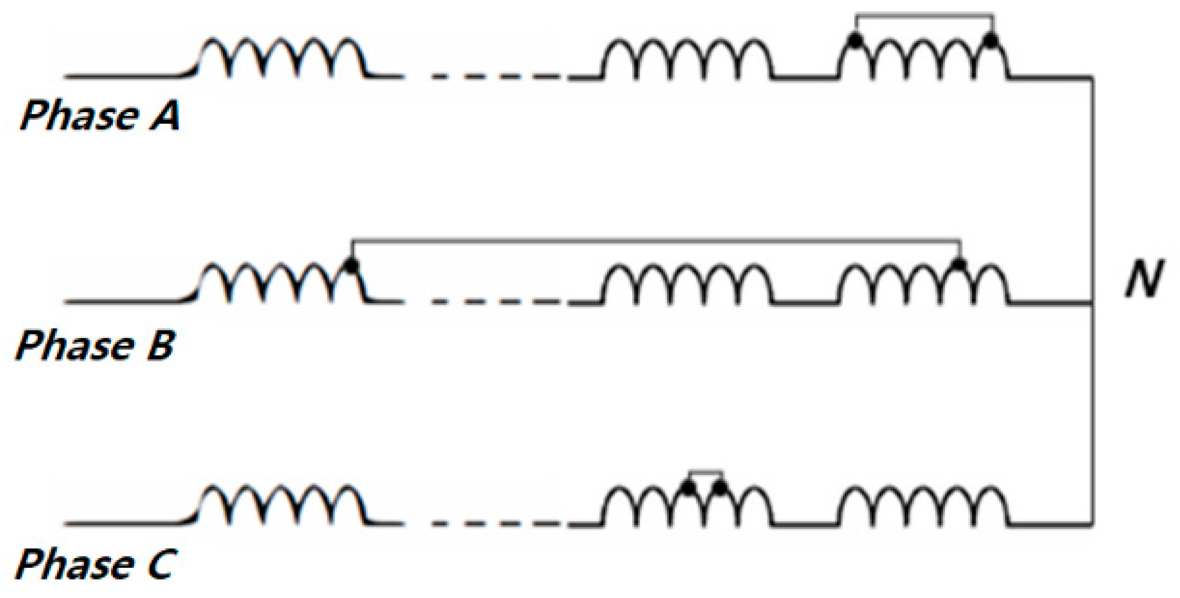
Figure 2.
Direct-quadrature (D-Q) transformation process: (a) D-Q stationary reference frame (b) D-Q synchronous reference frame.
Figure 2.
Direct-quadrature (D-Q) transformation process: (a) D-Q stationary reference frame (b) D-Q synchronous reference frame.
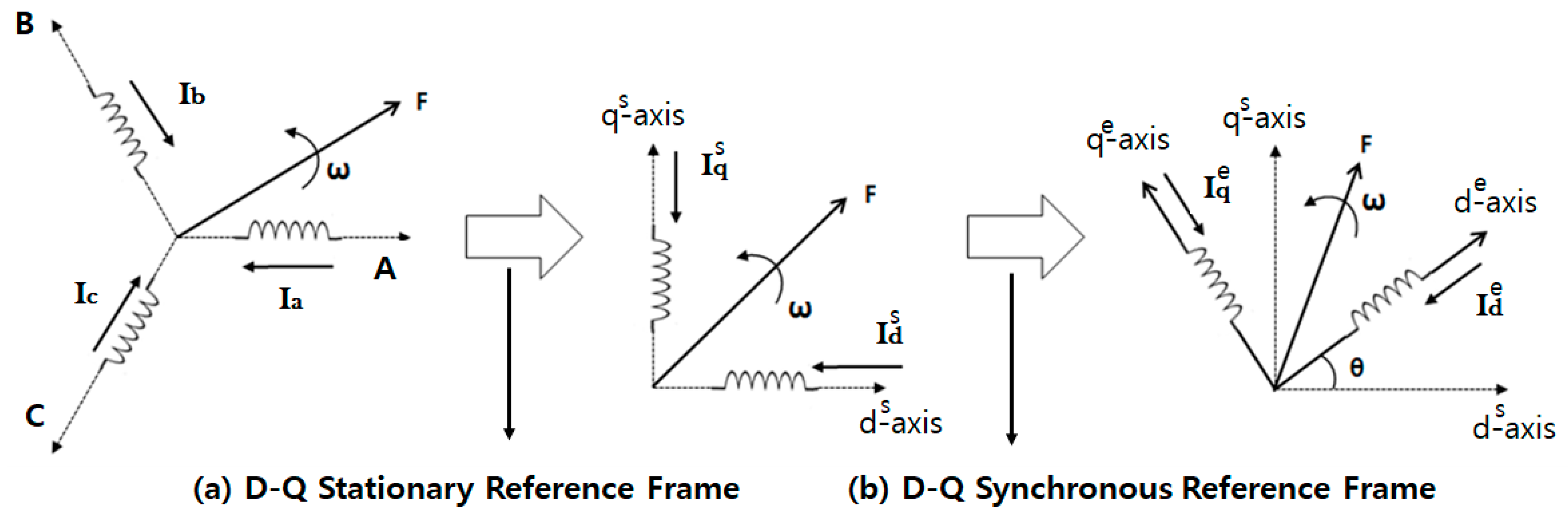
Figure 3.
Current change due to D-Q transformation (a) 3-phase input current, (b) D-Q stationary coordinate system, (c) D-Q synchronous coordinate system.
Figure 3.
Current change due to D-Q transformation (a) 3-phase input current, (b) D-Q stationary coordinate system, (c) D-Q synchronous coordinate system.
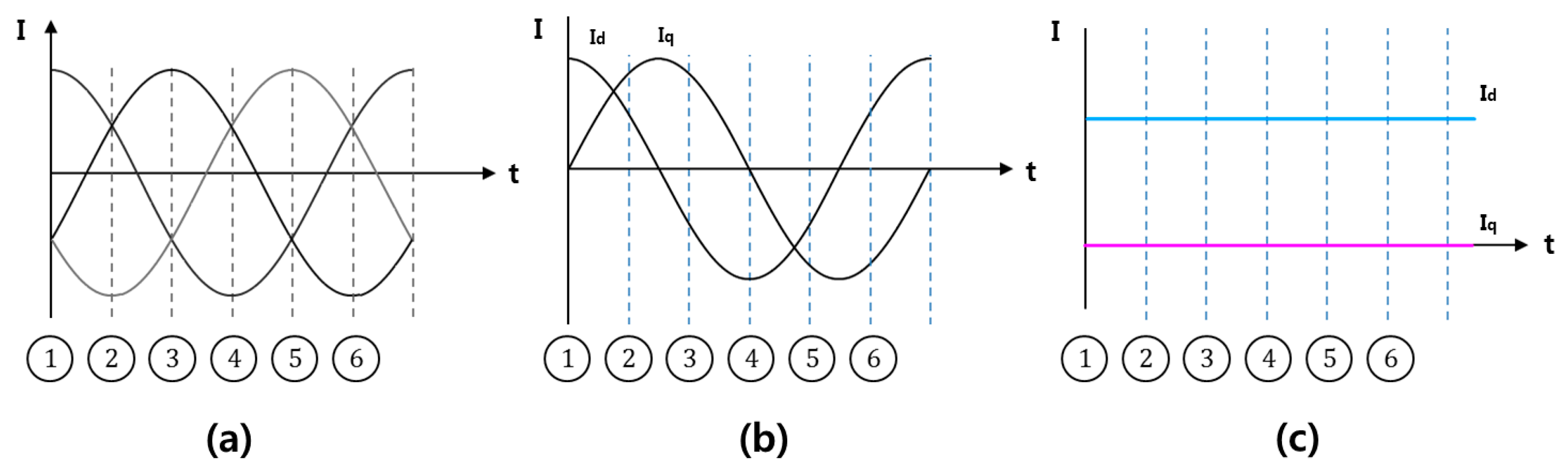
Figure 4.
(a) Turn short in phase A, (b) D-Q Transformation equivalent model by turn short circuit.

Figure 5.
(a) Definition of inductance and number of turns by turn short circuit and (b) two inductances due to turn short circuit.
Figure 5.
(a) Definition of inductance and number of turns by turn short circuit and (b) two inductances due to turn short circuit.
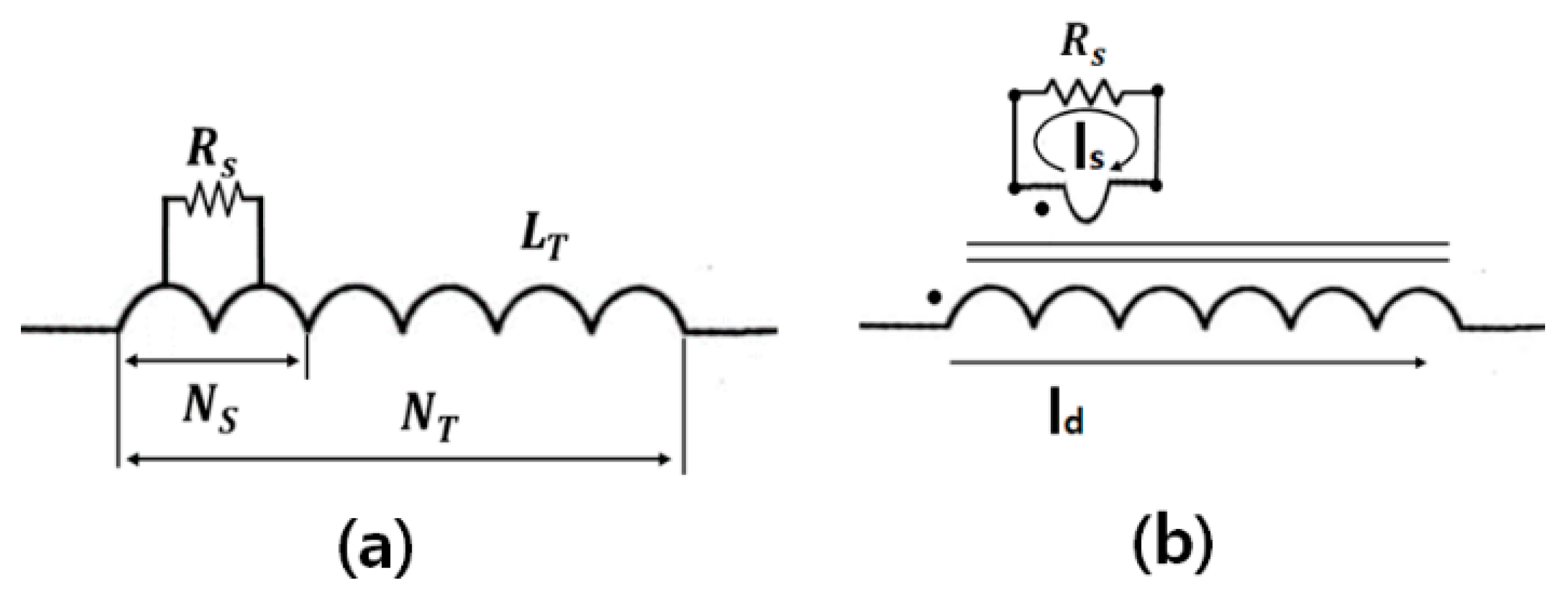
Figure 6.
Magnitude change of current with increasing turn short circuits.

Figure 7.
FAR–FRR interaction graph.
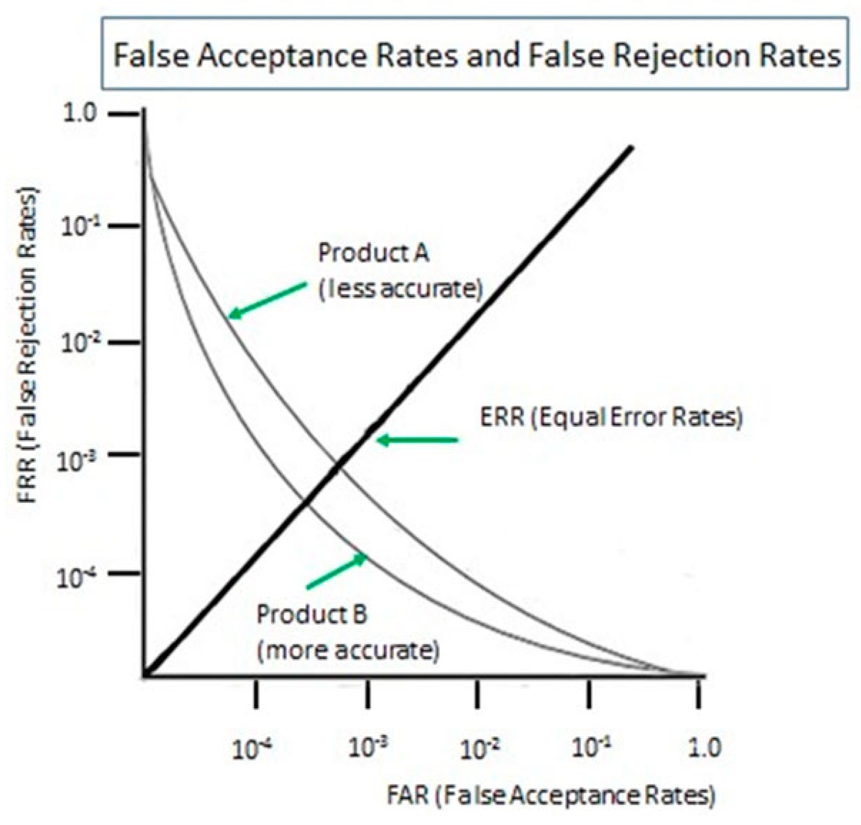
Figure 8.
Experimental device configuration.

Figure 9.
Filtering process for noise in the input power: (a) before filtering and (b) after filtering.
Figure 9.
Filtering process for noise in the input power: (a) before filtering and (b) after filtering.

Figure 10.
Method for configuring artificial turn short circuits: (a) short circuit of stator winding, (b) external tab of the turn short circuit motor.
Figure 10.
Method for configuring artificial turn short circuits: (a) short circuit of stator winding, (b) external tab of the turn short circuit motor.
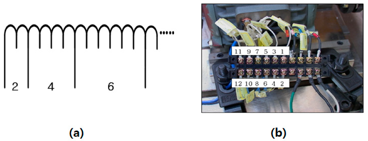
Figure 11.
D-Q synchronous coordinate system during the full short turn.
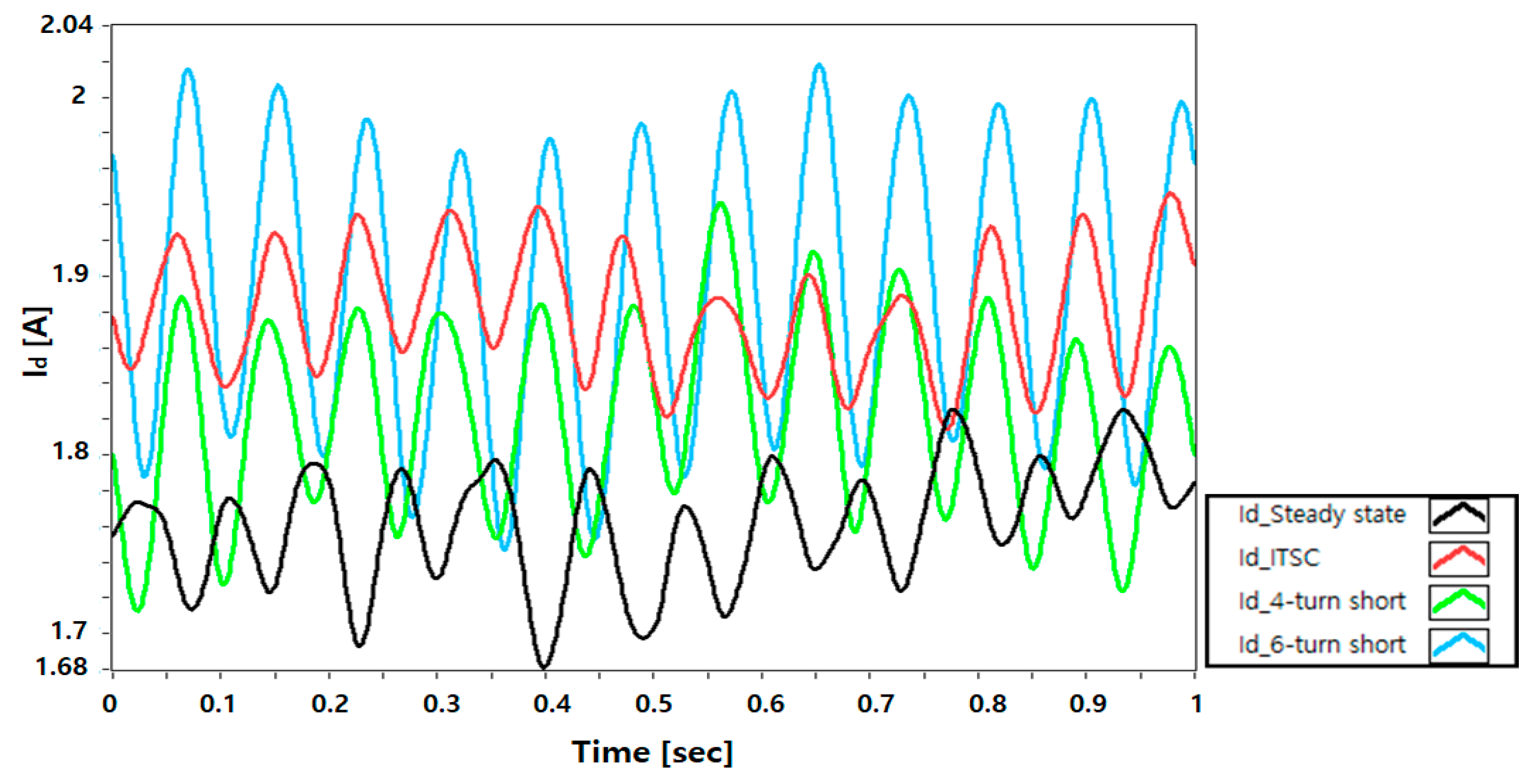
Figure 12.
D-Q synchronous coordinate system according to turn short circuit at no load.
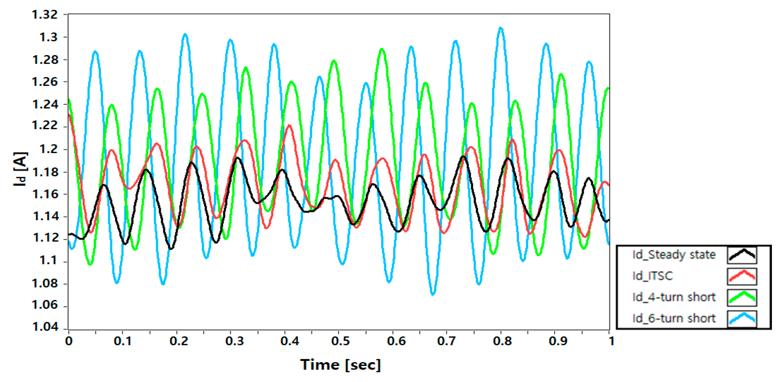
Figure 13.
D-Q min–max coordinate system according to the speed change.
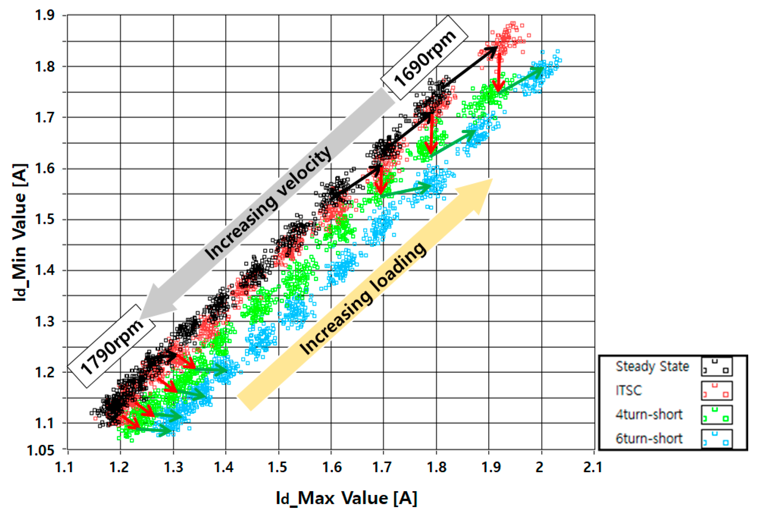
Figure 14.
Linear discriminant analysis (LDA) application and critical line according to general turn short.
Figure 14.
Linear discriminant analysis (LDA) application and critical line according to general turn short.

Figure 15.
LDA application and critical line according to inter-turn short circuits (ITSC).
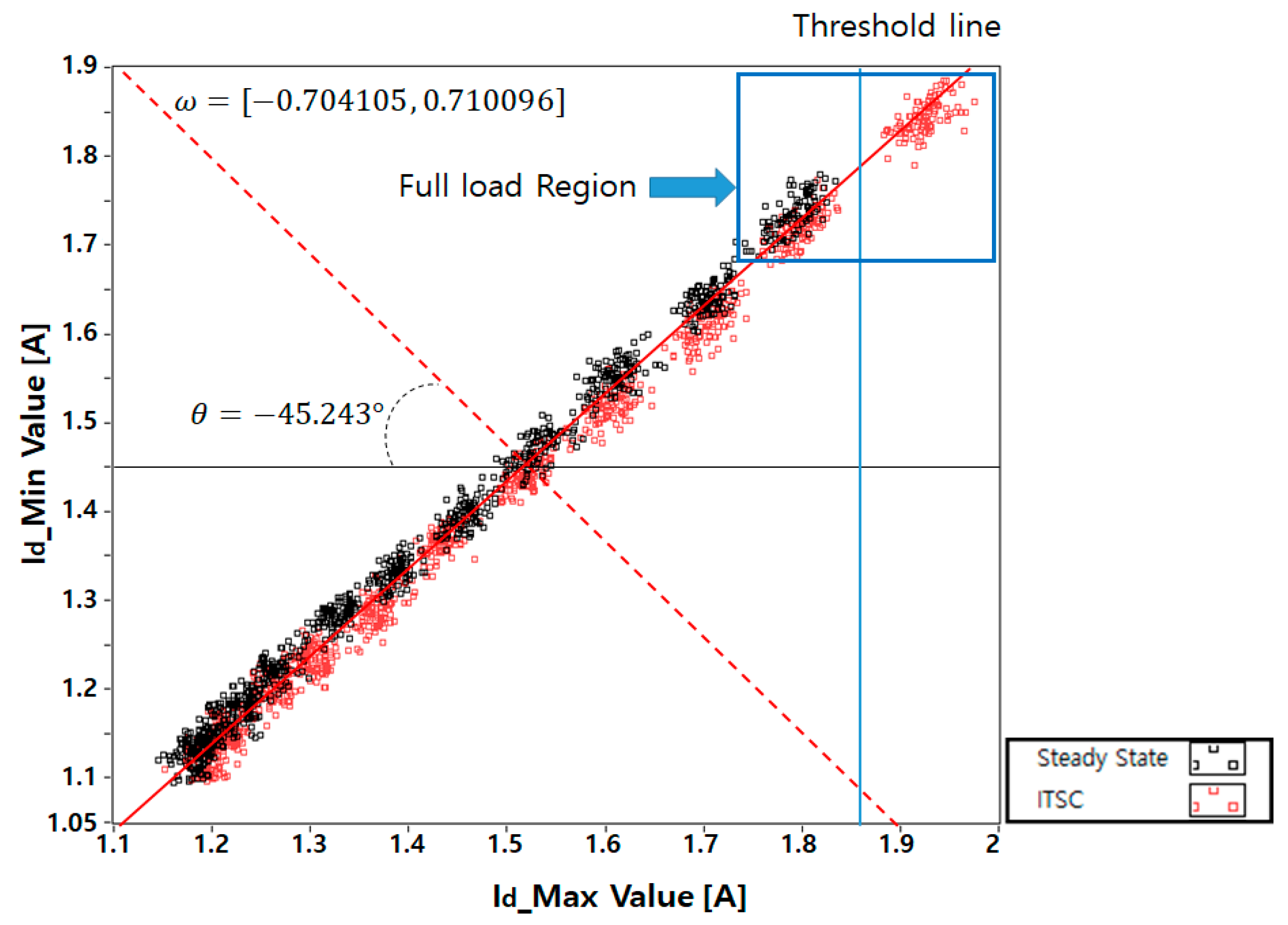
Figure 16.
Between-class scatter (BCS) in the steady-state and the ITSC state according to speed change.
Figure 16.
Between-class scatter (BCS) in the steady-state and the ITSC state according to speed change.
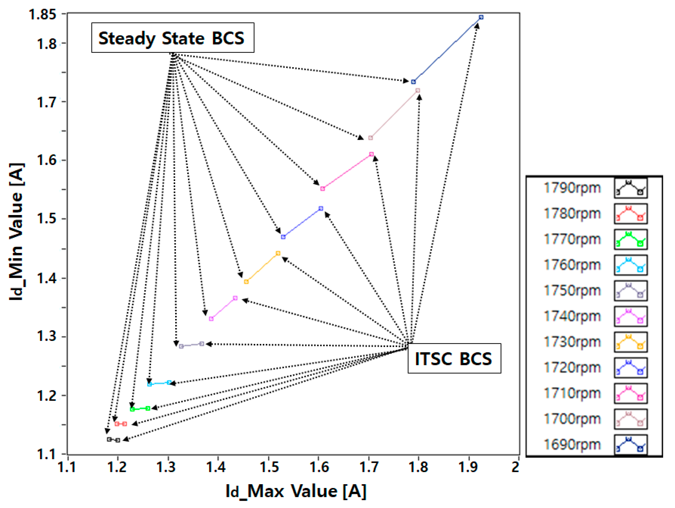
Figure 17.
False acceptance rate (FAR)–false rejection rate (FRR) graph at 1790 rpm.
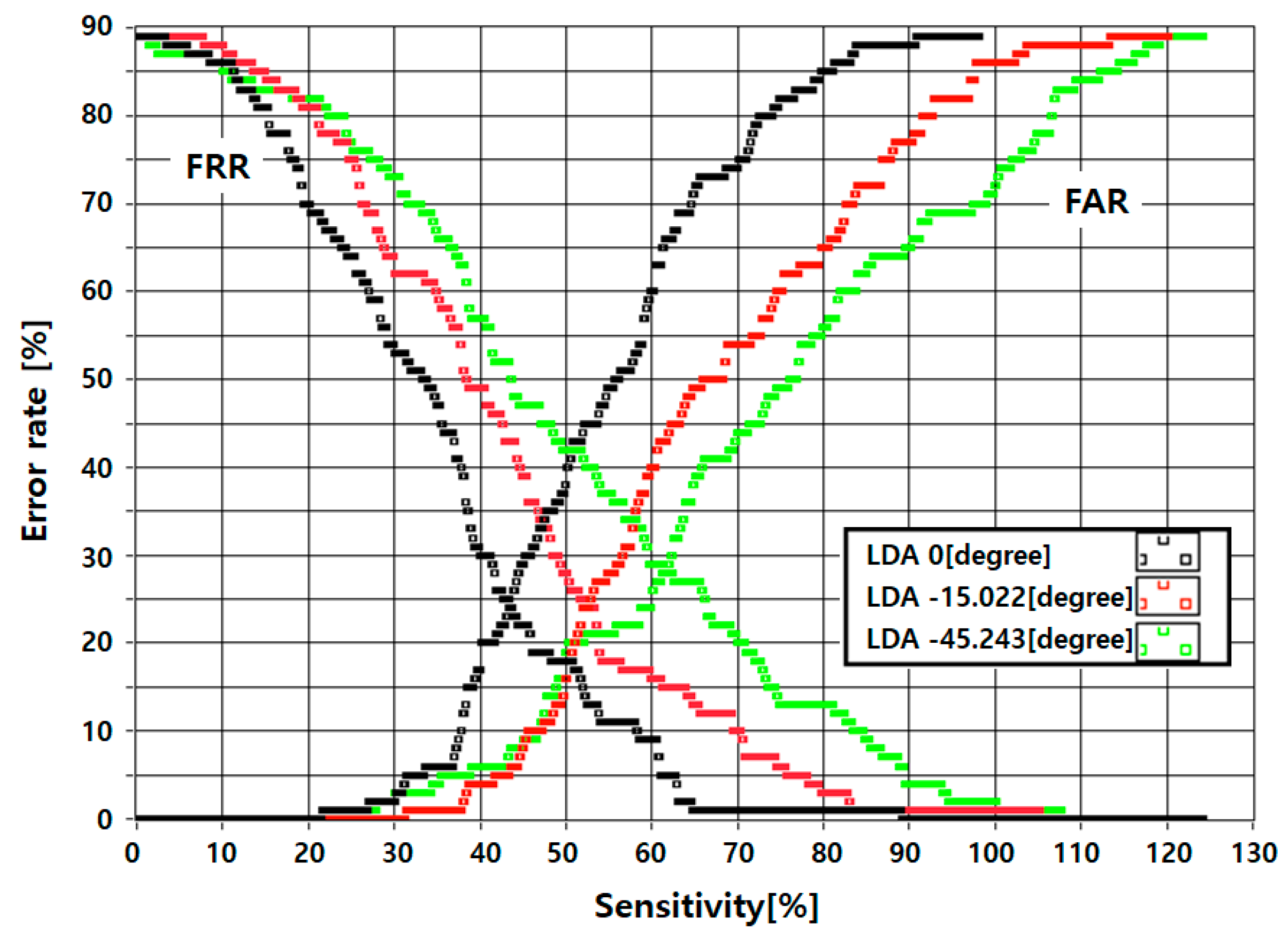
Figure 18.
FAR–FRR interaction graph at 1790 rpm.
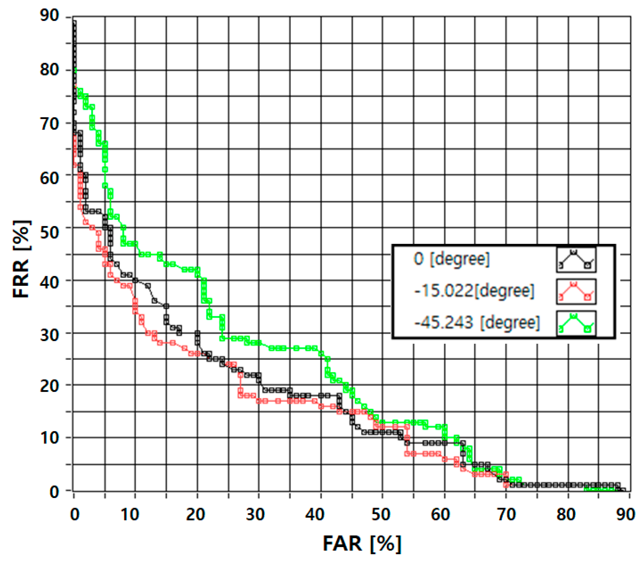
Figure 19.
FAR–FRR interaction graph when minimum light load LDA degree was applied to each speed.

Table 1.
Motor specifications.
| Description | Value |
|---|---|
| Power (kW) | 0.75 |
| Input Voltage (V) | 220/380 |
| Full Load Current (A) | 3.8/2.2 |
| Supply Frequency (Hz) | 60 |
| Number of Pole | 4 |
| Number of Rotor Slot | 44 |
| Number of Rotor Slot | 36 |
| Full Load Torque (kg·m) | 0.43 |
| Rated Speed (rpm) | 1690 |
Table 2.
Turn short fault.
| No. | 1–3 | 3–5 | 5–7 | 7–9 | 9–11 |
|---|---|---|---|---|---|
| Turn short | 2(ITSC) | 4 | 6 | 8 | 12 |
Table 3.
LDA direction information for each speed.
| Speed (rpm) | 1790 | 1780 | 1770 | 1760 | 1750 | 1740 | 1730 | 1720 | 1710 | 1700 | 1690 |
|---|---|---|---|---|---|---|---|---|---|---|---|
| Angle (Degree) | −15.02 | −18.40 | −16.88 | −15.45 | −14.51 | 7.421 | 6.341 | 5.765 | 8.652 | 13.66 | 13.2 |
© 2020 by the authors. Licensee MDPI, Basel, Switzerland. This article is an open access article distributed under the terms and conditions of the Creative Commons Attribution (CC BY) license (http://creativecommons.org/licenses/by/4.0/).
Share and Cite
MDPI and ACS Style
Goh, Y.-J.; Kim, K.-M. Inter-turn Short Circuit Diagnosis Using New D-Q Synchronous Min–Max Coordinate System and Linear Discriminant Analysis. Appl. Sci. 2020, 10, 1996. https://doi.org/10.3390/app10061996
AMA Style
Goh Y-J, Kim K-M. Inter-turn Short Circuit Diagnosis Using New D-Q Synchronous Min–Max Coordinate System and Linear Discriminant Analysis. Applied Sciences. 2020; 10(6):1996. https://doi.org/10.3390/app10061996
Chicago/Turabian StyleGoh, Yeong-Jin, and Kyoung-Min Kim. 2020. "Inter-turn Short Circuit Diagnosis Using New D-Q Synchronous Min–Max Coordinate System and Linear Discriminant Analysis" Applied Sciences 10, no. 6: 1996. https://doi.org/10.3390/app10061996
Note that from the first issue of 2016, this journal uses article numbers instead of page numbers. See further details here.