Porosity Prediction of Granular Materials through Discrete Element Method and Back Propagation Neural Network Algorithm


1
School of Highway, Chang’an University, South Erhuan Middle Section, Xi’an City 710064, Shaan Xi Province, China
2
Department of Civil and Environmental Engineering, Michigan Technological University, 1400 Townsend Drive, Houghton, MI 49931, USA
*
Author to whom correspondence should be addressed.
Appl. Sci. 2020, 10(5), 1693; https://doi.org/10.3390/app10051693
Submission received: 4 October 2019
/
Revised: 20 February 2020
/
Accepted: 26 February 2020
/
Published: 2 March 2020
(This article belongs to the Section Civil Engineering)
Abstract
:Granular materials are used directly or as the primary ingredients of the mixtures in industrial manufacturing, agricultural production and civil engineering. It has been a challenging task to compute the porosity of a granular material which contains a wide range of particle sizes or shapes. Against this background, this paper presents a newly developed method for the porosity prediction of granular materials through Discrete Element Modeling (DEM) and the Back Propagation Neural Network algorithm (BPNN). In DEM, ball elements were used to simulate particles in granular materials. According to the Chinese specifications, a total of 400 specimens in different gradations were built and compacted under the static pressure of 600 kPa. The porosity values of those specimens were recorded and applied to train the BPNN model. The primary parameters of the BPNN model were recommended for predicting the porosity of a granular material. Verification was performed by a self-designed experimental test and it was found that the prediction accuracy could reach 98%. Meanwhile, considering the influence of particle shape, a shape reduction factor was proposed to achieve the porosity reduction from sphere to real particle shape.
1. Introduction
Granular mixture is widely applied in industrial manufacturing, agricultural production and civil engineering, including powder metallurgy, food accumulation and building materials. For these mixtures, porosity is one of the most crucial factors that has a considerable impact on mixture structure and performance. However, due to the complex particle composition, it is hard to calculate or predict the mixture porosity without the help of lab experiments.
In order to solve the above problems, many researchers have proposed different methods to calculate and analyze the porosity of granular mixtures. In particuology, packing density calculation models based on the packing theory were derived, including the Furnas model [1], linear packing density model [2], compressible packing model [3] and other improved models [4,5]. All of them are analytical models which were used to analyze particle spatial distributions and mixture packing densities. However, some literature [6,7] confirmed that these models were not accurate enough for complex problems and where particles have a wide range of sizes. A typical mixture in pavement engineering, however, is mainly composed of mineral aggregates with a wide range of particles sizes. The fine aggregates are less than 2.36 mm while the large particles can be larger than 19.0 mm. Additionally, in pavement engineering, mixtures are formed through the lab or field compacting process which is dependent on the particle physical interactions. Evidently, these analytical models cannot consider the particle interactions during the compacting process. Based on the two considerations above, the authors believe that the conventional analytical models as discussed above are not applicable for predicting porosities of pavement mixtures.
In pavement engineering, experimental testing methods were popularly used for studying mixture porosities [8,9]. In the past decades, many research studies were conducted for building the relationship between porosities and compositions of mixtures, while most of them were applied to specific projects or limited conditions [10,11]. Since 2005, with the rapid development of the discrete element methods (DEM), virtual mixture models have been developed for studying mix porosities [12,13], where particle gradations and morphological features were considered. With the DEM-based study, the researchers tended to explore the relations between the mix porosity and its mix composition. However, in the existing literature, the research purposes were mainly focused on evaluating a limited number of mixtures instead of finding a universal model for predicting mixture porosities [14,15].
In the past decades, machine learning algorithms have been widely used to solve problems which have multiple variables with no clear relations. Various models have been developed in industrial design [16], disease diagnosis [17], engineering analysis [18], material optimization [19,20,21], etc., which validated the high accuracy and the universal application of machine learning algorithms. Back Propagation Neural Network algorithm (BPNN), which is a multilayer feedforward neural network trained according to the error back propagation algorithm, is one of the most widely used algorithms. There are some advantages to this method: strong nonlinear mapping ability, highly self-learning and adaptive ability, good generalization ability and certain fault-tolerant ability. In recent years, some research efforts have been made in asphalt pavement engineering to study asphalt mixture’s volumetric properties, gradations and asphalt contents with the BPNN [20,22,23]. Additionally, the BPNN-based methods were also used for the prediction of cement concrete compression strength [24,25,26]. As demonstrated in the literature, the BPNN was useful and efficient in solving asphalt or concrete pavement problems.
Obviously, the BP models have advantages for predicting mixture porosities. However, a reliable database which has enough data is one of the key requirements for using such a BP model. It is hard to obtain such a consistent database with the traditional experimental methods since their testing results are dependent on the testing methods, materials, specification and so on. One advantage of the DEM-based modeling approaches is lab-independent. First of all, with the DEM model, users can control one or a few key factors without effects from the other factors. For instance, it is possible to build a DEM model of mixture where all the particles have identical shapes if one wants to explore effects of gradations without influences of particle shapes. As a result, it is possible to obtain consistent results which stick to certain conditions. Secondly, limited by materials and testing conditions, it is very difficult to obtain a large amount of consistent experimental data. With the DEM model, however, it becomes possible to obtain a large amount of data as long as one has the DEM modeling techniques and computer facilities.
Against the background discussed above, the main objectives of this research are to explore the prediction of granular materials’ porosities by combining the DEM simulation and the BPNN methods. The granular materials in this research refer to mineral aggregates whose sizes range from 2.36 mm to 19 mm. They are key constituents of asphalt mixtures which take over 90% of the overall mass and their porosities may significantly impact mixture volumetric and mechanical properties [27,28]. Compared to aggregates, asphalt acts more like lubricant during the compaction stage and its impact to mixture porosity can be ignored in this article [12,29]. According to the Chinese specifications, mixtures whose maximum particle sizes are from 13.2 mm to 19.0 mm are popularly used as high-quality pavement construction. As demonstrated in the previous research [13,30], both gradations and particle shapes could have certain impacts on mixture volumetric properties. When both gradations and particle shapes are considered simultaneously, it is not easy to make a consistent conclusion. Therefore, in this article the aggregate gradations were selected as the major control parameters, while the particle shapes were considered as minor parameters by introducing a reduction factor.
2. Training Data Acquisition Based on Virtual Compacted Particle Mixtures
2.1. Coarse Aggregate Proportion Database
2.1.1. Determination of Possible Gradation Scope
In order to contain all possible proportions of coarse aggregates from 2.36 mm to maximum particle size, the recommended range of each particle size group was summarized on the basis of Chinese Construction Specification JTG F40-2004 [31], including various common gradation types: asphalt concrete (AC), asphalt macadam (AM), open graded friction course (OGFC) and stone mastic asphalt (SMA). In this way, the maximum possible gradation scopes of different maximum nominal particle sizes are obtained finally, as shown in Table 1 and Table 2.
It could be observed that the mineral mixtures had a large particle size polydispersity, but the particle size ratios in each sieving size group in pavement materials were relatively small. However, the particle size distribution of the mixture can be adjusted by changing the proportion of sieving groups.
2.1.2. Establishment of Coarse Aggregate Proportion Database
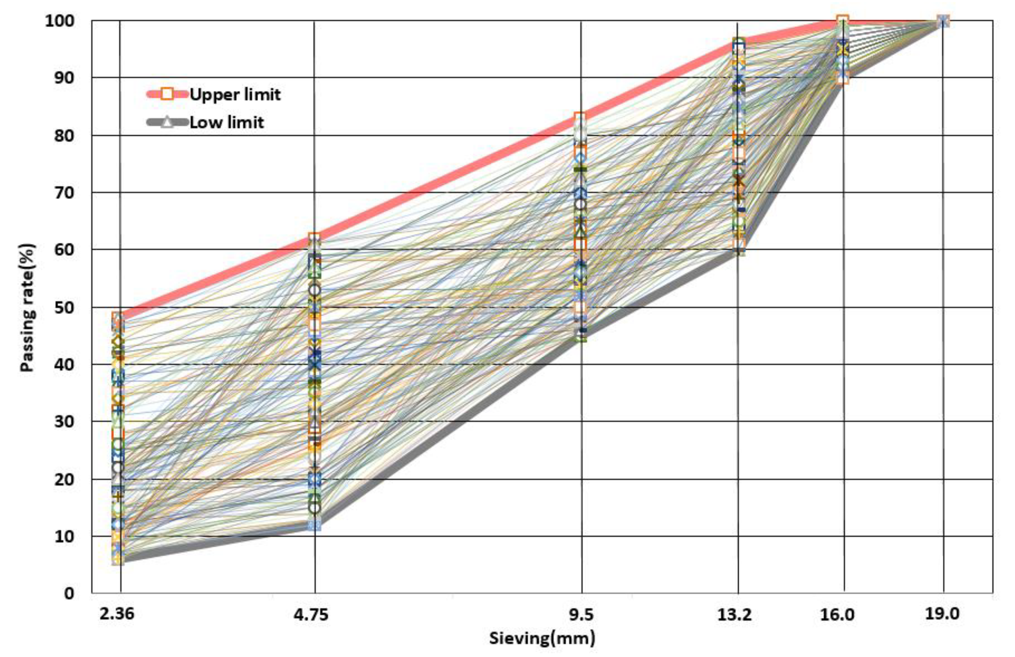
Machine learning algorithms require large sample size to ensure the stability and accuracy or prediction results. In order to obtain enough test data for training for both Gradation-13 and Gradation-16, 200 coarse aggregates’ proportions were randomly created by VBA within the upper and lower limit listed in Table 1 and Table 2. As shown in Figure 1 and Figure 2, 200 combinations cover almost all possible gradations between upper and lower limit for one gradation type.
In the above two figures, the upper and lower rough lines represent the upper and lower bounds of the gradation. Meanwhile, each fine line in the middle of upper and lower limits represents a particle combination. Although particle compositions cannot be listed completely, figures justify that the samples used for model training are representative.
2.2. Virtual Compacted Model Design
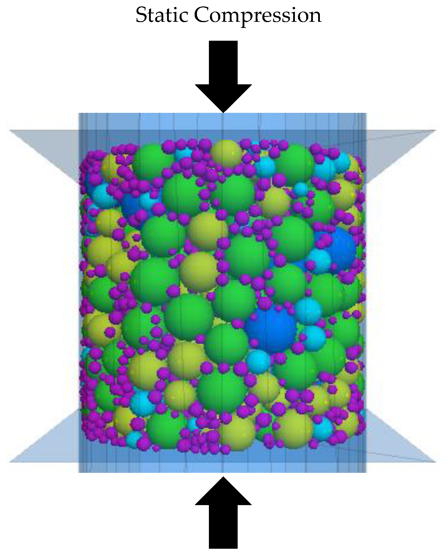
In this study, Particle Flow Code (PFC) was applied to carry out the virtual compaction test. Static compaction, as a commonly used compaction method in road material’s DEM modelling, was chosen, considering both compacting effect and computing efficiency. In addition, in order to determine a suitable static compaction pressure, the influence of static pressure applied for the compaction was tested in detail. It should be noted that all particles are ball shaped in order to control a single variable in this stage. Three gradations were selected randomly and their passing rates are shown in Table 3.
Since all the particle combinations were a coarse part of an entire gradation, the total mass of different mixtures may also be different. All elements were generated in accordance with passing rate and total volume of design specimen. The boundary condition for the container is simulated by a wall, which is similar to its counterpart steel container in the laboratory test. The compaction pressure only applied on top and bottom wall. The height of design cylindrical specimen is 100 mm and the diameter of the container is also 100 mm.
For each specimen, the virtual test mainly follows three steps:
- (1)
- The ball elements were generated without overlap in a random position in a cylindrical area;
- (2)
- Seven levels of hydrostatic pressure were applied to compact seven specimens, including 100 kPa, 200 kPa, 300 kPa, 400 kPa, 500 kPa, 600 kPa and 700 kPa;
- (3)
- Compression was performed until all elements become stable as shown in Figure 3. At that time, mixtures are considered to be in the most compact state.
Because there are only coarse aggregates in this model, linear contact model was applied to all particles. The density of aggregates was set as 2650 g/cm3 and effective modulus and friction coefficient were 50 GPa and 0.4, respectively. The results are shown in Table 4.
It can be observed that compaction pressure caused little effect on final porosity for same gradation mixture. Taking Gradation#1 as an example, the range of mixture porosity is from 0.328 to 0.334, which indicates the mixture with sphere particles can be well compacted at all above pressures. Meanwhile, a compaction pressure of 600 kPa is commonly used in laboratory tests in many countries’ specification, for instance, Superior Performing Asphalt Pavement (SUPERPAVE) specification. Therefore, a fixed compaction pressure of 600 kPa was chosen to carry out virtual compaction tests in this study. The particle number in each specimen varies from about 1000 to 17,000 for different gradations, and computing time changes from 10 min to nearly 2 h.
2.3. Data Recording
Through above virtual compaction models, the porosity of coarse aggregates (larger than 2.36 mm) mixtures were measured and recorded. In order to eliminate the impact of contingency, three gradations were randomly selected and five parallel virtual experiments were conducted. In each group of parallel virtual experiments, the particle size distributions were identical, but the initial positions of ball elements were different. The detailed results are shown in Table 5.
According to the results, it can be observed, that for the same gradation, the porosity measured by different parallel specimens is very close. However, there are great differences among different gradations, which shows that the results of the virtual compaction test were credible. Therefore, the porosity of Gradation-13 and Gradation-16 specimens were recorded respectively in the same way. The following Table 6 and Table 7 show the final results of two types of gradation.
Based on above data, the internal relationship between independent variables (retained percentage of each particle size group) and dependent variable (porosity) will be further analyzed in the next chapter.
3. Data analysis and BP Neural Network Model Building
MATLAB software included plenty of useful functions of neural network algorithm in the Neural Network Toolbox as shown in the literature [32]. These functions provide the possibility to build a basic model for those not professional at machine learning. Therefore, the BPNN models in this article were built with “newff” function in Neural Network Toolbox of MATLAB, which is easy for reference.
In general, the BP neural network model includes an input layer, an output layer and multiple hidden layers. The previous research shows that the three layer BP neural network with one hidden layer can approximate any non-linear function [32]. Hence, the model in this article was established with one hidden layer and the model structure is shown in Figure 4.
In the BP model, there are three kinds of key parameters: (1) input and output variables; (2) transfer function; (3) the number of hidden layer nodes and their corresponding weight thresholds. Through the above three parameters, a complete BP neural network prediction model can be obtained and calculated through Equation (1).
where (1) represents model input variables (particle volume fraction of different particle size groups); represents model output result; k represents the number of input variables in the range of 1 to m; m represents the total number of input variables, four for Gradation-13 and five for Gradation-16; (2) refers to transfer function; (3) i represents the number of hidden layer nodes in the range of 1 to n; n refers to the total number of hidden layer nodes; represents weight from input layer to hidden layer; refers to weight from hidden layer to output layer; represents threshold from input layer to hidden layer; represents threshold from hidden layer to output layer.
In addition, in order to evaluate model training accuracy, Mean Square Error (MSE) and coefficient of determination () of the output results are applied and MSE can be calculated according to Equation (2).
where represents the test value and represents the real value. Meanwhile, n refers to the test set sample number.
In “newff” function, there are not too many parameters to be determined. Hence, all of them are listed in the following Table 8.
Because of the high relativity between gradation and mixture porosity, the prediction accuracy was great enough when the default functions were applied. In order to simplify the procedures of building the prediction model, the default transfer functions were finally determined. It should be noted that the determination of other key parameters is illustrated in the following Chapter 3.1, Input and output variables processing.
3.1. Input and Output Variables Processing
For the model in this article, the input layer contains four variables (i.e., particle volume fraction of 13.2–16.0 mm, 9.5–13.2 mm, 4.75–9.5 mm and 2.36–4.75 mm) for Gradation-13 and five variables for Gradation-16, and output layer includes the only dependent variable, porosity, for both gradation types.
The first and foremost step in BP neural network modeling is to process the original input data. Because the recorded data are relatively close to each other in the whole range of 0.30–0.45, it is necessary to standardize the original data and transfer variables into the range of [–1, 1] according to Equation (3). Meanwhile, the original gradation should also be processed through Equation (3). This procedure can achieve the best performance for modeling.
where and represent 1 and −1 respectively in this article, while and refer to the maximum and minimum value of recorded porosity and refers to original porosity, while refers to standardized porosity.
Through the above equation, the procedure for standardizing the input variables includes these three parts: (1) finding maximum and minimum values in the recorded porosity as and ; (2) calculating each standardized porosity () value through Equation (3); (3) recording standardized porosity () values.
The next step is to divide the available data set into two groups, one for training and another for testing the developed model. Meanwhile, the testing set will not be used in the model training process. It should be noted that grouping is done randomly. In this study, 200 particle compositions and corresponding porosity for both Gradation-13 and Gradation-16 were randomly divided into training and testing groups.
Finally, the output results still need to be anti-standardized in a similar way by following Equation (4):
where, and refer to the maximum and minimum value of recorded porosity and refers to prediction porosity, while refers to standardized prediction porosity.
The standardized and anti-standardized can be completed automatically by function “mapminmax” in MATLAB only if the original data is inputted.
3.2. Transfer Function Determination
There are three transfer functions commonly used in the BP neural network model and these functions are applied in the hidden and output layer. The default transfer functions in “newff” function include a hyperbolic tangent function(“tansig”) in hidden layer as shown in Equation (5) and a pure linear function(“purelin”) in the output layer in Equation (6).
The final prediction formula can be obtained by training the model to determine the appropriate parameters. Among these parameters, the number of hidden layer nodes should be tested by user. The other corresponding parameters could be determined automatically.
3.3. Hidden Layer Node Number Determination
Generally, the model accuracy will be improved by increasing the training sample size. However, when the sample size is large enough, even more data cannot improve the model performance. For the purpose of studying the relationship between original sample size and training model performance, different training sample sizes were tested and compared. The mean square error (MSE) and coefficient of determination (R2) between prediction value and virtual test value were calculated to evaluate the accuracy and stability of final prediction model. Seven models for Gradation-13 were built in this article with sample sizes of 25, 50, 75, 100, 125, 150 and 175 respectively. For all seven models, 25 samples were applied as the testing group to check the model performance by calculating R2.
For the BP model, except for training sample size, the hidden layer node number also plays a significant role in model training. According to empirical Equation (7), the range of node number is set as 3 to 13.
where, m and n refer to the number of input and output layer nodes respectively and a refers to a regulating constant in the range of 1 to 10. For each group, 10 parallel tests were carried out to determine the optimum node number. The detailed procedure is omitted in this article since it was introduced in another publication [32]. The following Figure 5 shows that coefficient of determination (R2) changes with node number.
It can be observed that: (1) the optimum node number can be different for different models; (2) with training sample size increasing, model performance is less sensitive to node number. The optimum hidden layer node number for all seven groups are shown in the following Table 9.
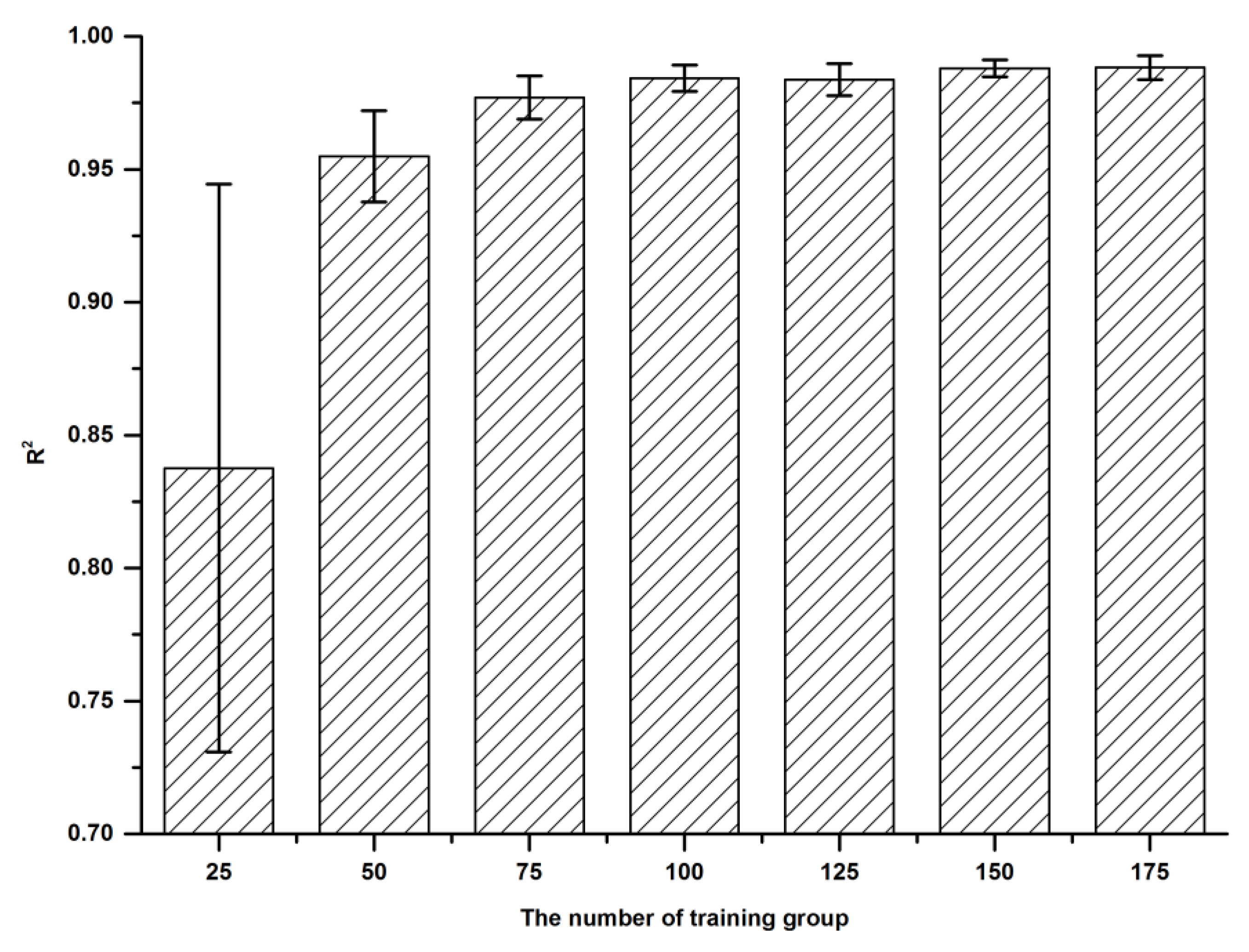
Meanwhile, the following Figure 6 shows the R2 for different models based on their optimum node number. The error bars here represent standard deviation.
From this figure, it is clear that with the increase of training group sizes, R2 rises sharply in the initial stage. After the number of training groups goes up to more than 75, the growth rate of R2 becomes very small. Meanwhile, for model accuracy, when the amount of training data is too small, the model error is very large. With the increase of training data size, the model tends to be more stable. In this state, a more accurate prediction model can be obtained.
Based on the above analysis, the number of training sets was recommended as 75 or 100, considering training accuracy and efficiency. Meanwhile, the best number of testing sets is about 1/2–1/3 of the training set.
3.4. Testing Results
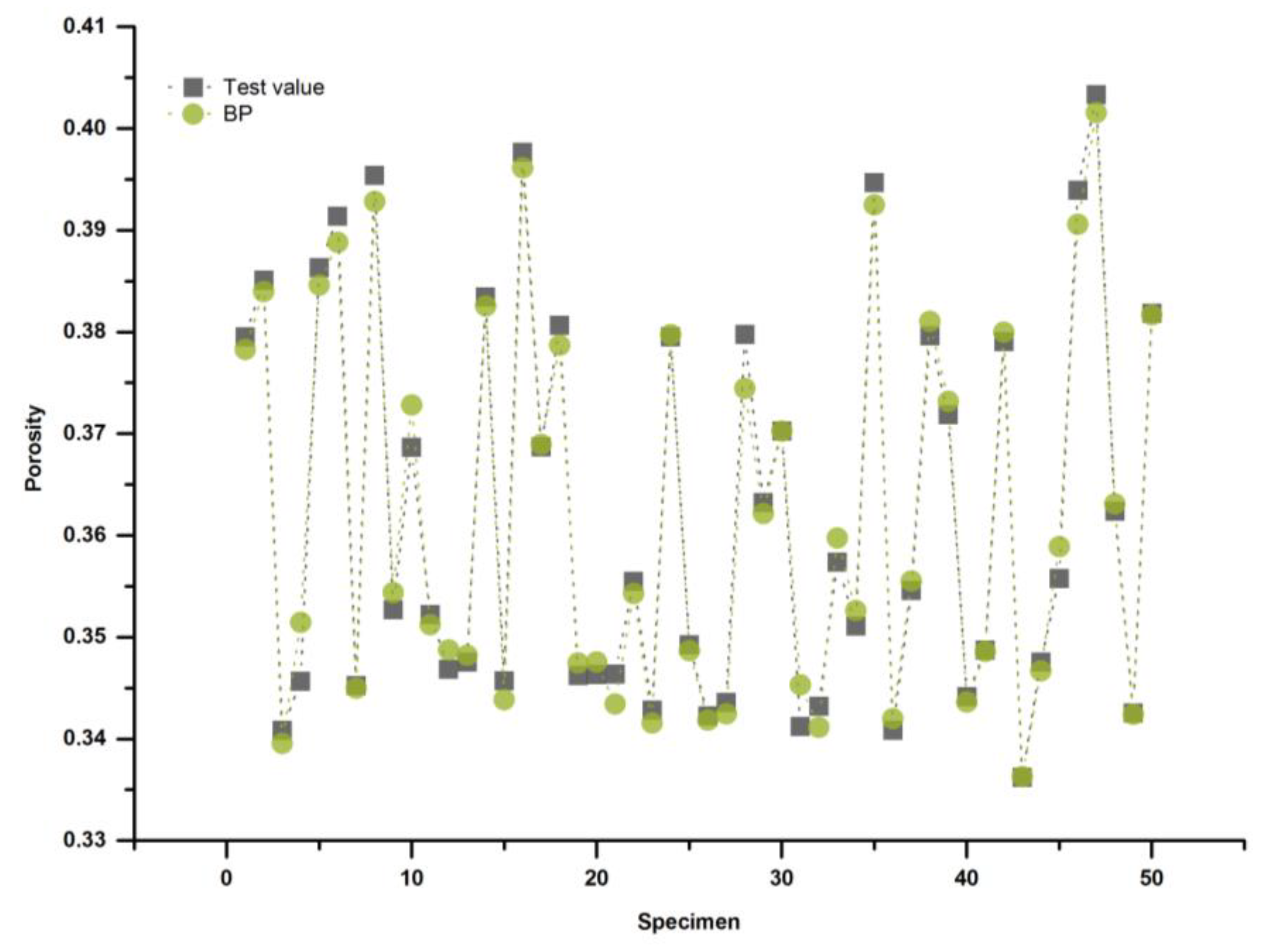
On the basis of the existing database, 150 groups were used as the training group and 50 groups were applied as the testing group to build the BP neural network model. The training results are shown in Figure 7 for Gradation-13 and Figure 8 for Gradation-16.
In the process of data transmission, through repeated training, four hidden layer nodes for Gradation-13 and five nodes for Gradation-16 were finally determined as the most suitable number of hidden layer nodes.
For two models, their coefficients of determination both achieve 99%, which means porosity prediction models have enough accuracy to provide reliable results.
In addition, all the related parameters applied in model training are listed in the following tables. Table 10 and Table 11 provide the gradation and porosity normalization parameters ( for Gradation-13 and Gradation-16. Through these parameters, the original gradation and porosity data could be normalized according to Equation (3). Then, the weights and thresholds used to transfer data from the input layer to the hidden layer are shown in Table 12, while those parameters from the hidden layer to the output layer are shown in Table 13.
The complete prediction calculation process is listed as follows:
- Step1: Original gradation and porosity data are recorded and inputted to MATLAB program.
- Step3: The values in hidden layer are calculated according to Equations (8).
- Step4: The values in output layer are calculated according to Equations (9).
- Step5: The calculated results are anti-normalized through Equation (4).
Through the above steps, the porosity of a certain kind of particulate mixture can be accurately predicted.
4. Verification and Application of Prediction Method
For the purpose of evaluating model validity and accuracy, a static compression test was also completed in laboratory. The steel balls were used to compare with the virtual ball element model. Meanwhile, the relationship among the measured porosity, the simulated porosity and the predicted value was compared. In order to simulate the real composition of granular particles applied in highway engineering, a great number of steel balls in different sizes were prepared and mixed in the same proportion as uniformly as possible, then sieved to several different size groups. The original particle size distribution and sieved results of the steel balls are shown in Table 14 and Figure 9.
According to Table 14 and Figure 9, every sieving group was mixed with several different particle size groups uniformly. For 9.5–13.2 mm group, 13.0 mm particles were not found, so 12.303 mm balls were added to keep a continuous and real size distribution in the steel balls.
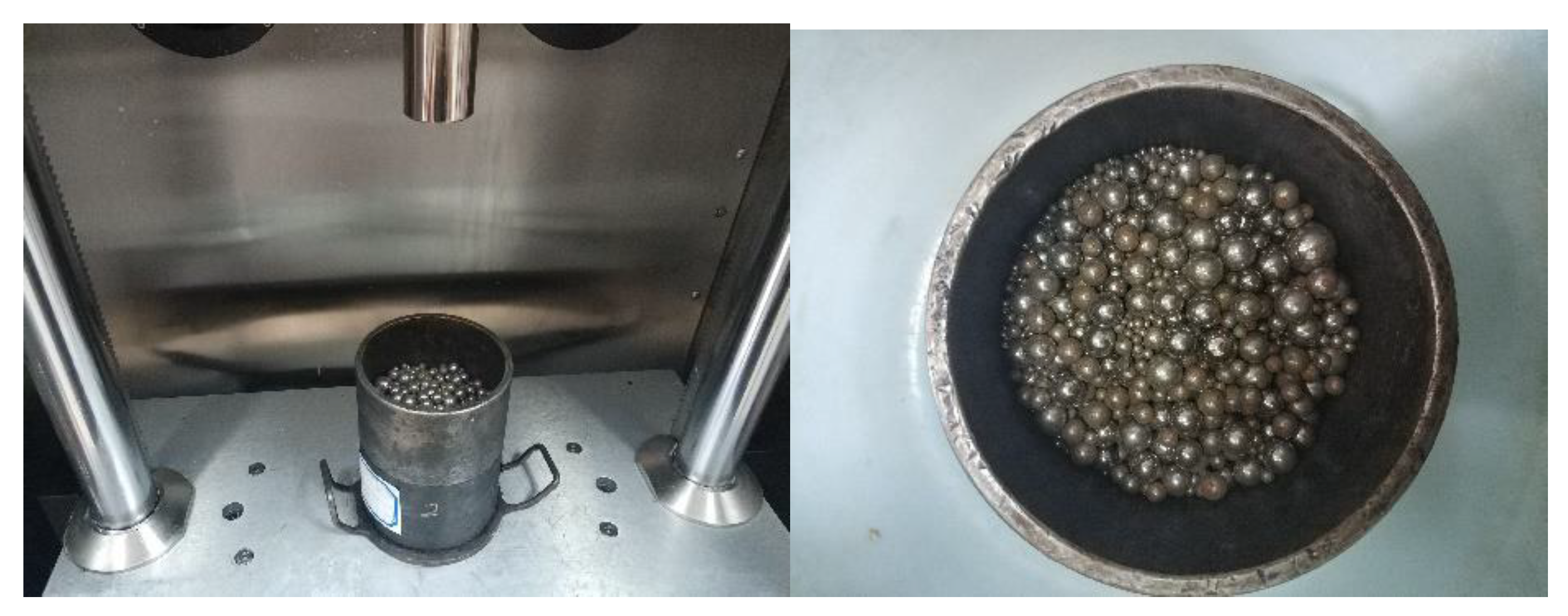
Then, in order to make the results of laboratory and DEM comparable, the size of steel ball experiments’ container was exactly the same as the DEM model. According to different gradations, the steel balls were mixed in a standard Marshall mold, whose diameter was 100 mm as shown in Figure 10. Because there was no filler or binder in this mixture, universal testing machine were applied to compact the mixed steel balls with a static pressure of 600 kPa. Meanwhile, particles’ total volume was measured by the displacement method. On the other hand, virtual compression tests on computer and porosity prediction on BP neural network model were completed at the same time. The detailed test data is shown in the following Figure 11.
As can be seen from the above figure, model prediction accuracy for the steel ball test was very high and model error was extremely slight. The maximum relative error of prediction was no more than 1.15%. This proved the credibility of the prediction model. Meanwhile, the results of lab tests and virtual tests were very close, which also proved that for the sphere element-based model, sufficient credible raw data could be obtained by DEM.
5. Reduction Factor Analysis Considering Particle Shape Effect on Mixture Porosity
From the above illustration, a porosity prediction model for sphere element has been established. However, as mentioned in the Introduction, paving materials in reality generally have complex but similar particle shape combinations, which indicate that shape effect is non-negligible but consistent. Therefore, a reduction factor to consider particle shape effect was introduced in this chapter.
A gradation was selected randomly for comparing the mixture porosity between sphere elements model and real aggregate shape model. The volume of each particle size group was:
A total number of 15 DEM models with different real aggregated shapes were built based on previous researches [33,34,35,36,37]. It should be noted that there is only one particle shape in each specimen to amplify its effect, as shown in Figure 12.
All the aggregate shapes used in this chapter were quite common. Although there are some special shapes in civil engineering, for instance, elongated particle, their volume percentages in mixture were generally low and strictly controlled, due to their poor engineering properties. The model parameters were identical with sphere element-based models. In this way, these mixtures’ porosities were recorded and plotted on the following Figure 13.
From Figure 13, the red line represents the mixture porosity of the sphere elements-based model, which was 0.381, while the green points refer to 15 mixture porosities in 15 real aggregate shapes respectively. It can be observed that there is an obvious difference between these two models. Nevertheless, this difference is quite stable and consistent among 15 green points. Detailed statistical analysis has been done as shown in the following Table 15.
From Table 15, 95% confidence interval has been determined and plotted as shown in Figure 13. Therefore, a shape reduction factor range was recommended considering the shape effect through Equations (10) and (11).
When the prediction results based on sphere element models are multiplied by shape reduction factor, a more accurate result could be obtained.
6. Summary and Conclusions
In this research, a porosity prediction model was established for granular mixtures through the DEM model and BPNN algorithm. A total of 400 mixes were simulated with the discrete element method to provide the database for BPNN training and testing. The prediction results were verified by steel ball experiments. Through this research, the following findings and conclusions were observed:
- This study provided an efficient and detailed method to build a porosity prediction model according to DEM model and BPNN algorithm. After model training, testing in MATLAB and verifying in lab experiments, the model’s coefficients of determination could achieve 99%.
- A suitable original database size was compared and recommended: prediction model accuracy could reach about 98% when the original data size was larger than 75. The amount of raw data can be determined according to different accuracy requirements.
- A shape reduction factor was proposed to achieve the porosity reduction from sphere to real particle shape, which made the porosity prediction results closer to reality and easy to use. In this research, particle shapes were not considered as the primary control parameters, which will be considered in a future study. Evaluation is recommended of particle shapes through combining the findings of this research with experimental testing methods.
Author Contributions
Conceptualization, Y.L.; Data curation, M.L.; Funding acquisition, Y.L.; Methodology, M.L.; Resources, B.M.; Software, P.S.; Supervision, Z.Y.; Validation, P.S.; Writing—original draft, M.L.; Writing—review & editing, Y.L. and P.S. All authors have read and agreed to the published version of the manuscript.
Funding
This research was funded by National Natural Science Foundation of China, grant number 51978074. The APC was funded by National Natural Science Foundation of China.
Conflicts of Interest
The authors declare no conflict of interest. The funders had no role in the design of the study; in the collection, analyses, or interpretation of data; in the writing of the manuscript, or in the decision to publish the results.
References
- Furnas, C.C. Grading aggregates, i. Mathematical relations for bed of broken solids of maximum density. Ind. Eng.Chem. 1931, 23, 1052–1058. [Google Scholar] [CrossRef]
- Stovall, T.; Larrard, F.D.; Buil, M. Linear packing density model of grain mixtures. Powder Technol. 1986, 48, 1–12. [Google Scholar] [CrossRef]
- Li, W.; Zhang, B.; Li, P. Application of particle packing model in concrete. J. Shenzhen Univ. Sci. Eng. 2017, 34, 63–74. [Google Scholar]
- Roquier, G. The 4-parameter Compressible Packing Model (CPM) for crushed aggregate particles. Powder Technol. 2017, 320, 133–142. [Google Scholar] [CrossRef]
- Roquier, G. A Theoretical Packing Density Model (TPDM) for ordered and disordered packings. Powder Technol. 2019, 344, 343–362. [Google Scholar] [CrossRef]
- Moutassem, F. Assessment of packing density models and optimizing concrete mixtures. Int. J. Civ. Mech. Energy Sci. 2016, 2, 29–36. [Google Scholar]
- Xiao, B.; Yang, Z.; Gao, Q.; Guo, X. Discussion on packing density models of combined aggregate and a new solution. Mater. Rep. 2018, 32, 2400–2406. [Google Scholar]
- Xu, X. Study on the voids in coarse aggregate by means of vibration molding based on the uniform experiment. J. Wuhan Univ. Technol. Transp. Sci. Eng. 2016, 40, 615–618. [Google Scholar]
- Chen, Q.; Li, Y. Test research on influence pattern of mineral aggregate’s gradation on volume properties of the exterior layer asphalt mixture. J. Wuhan Univ. Technol. Transp. Sci. Eng. 2011, 35, 71–75. [Google Scholar]
- Jiang, W.; Sha, A.; Xiao, J.; Li, R. Prediction model of air void content for porous asphalt concrete. J. Wuhan Univ. Technol. 2011, 33, 55–59. [Google Scholar]
- Jiang, W.; Sha, A.; Xiao, J.; Wang, Z. Gradation optimization of porous asphalt mixtures based on rutting resistance. J. South China Univ. Technol. Nat. Sci. Ed. 2012, 40, 127–132. [Google Scholar]
- Shen, S.H.; Yu, H.N. Analysis of aggregate gradation and packing for easy estimation of hot-mix-asphalt voids in mineral aggregate. J. Mater. Civ. Eng. 2011, 23, 664–672. [Google Scholar] [CrossRef]
- Li, J.; Zhang, J.H.; Qian, G.P.; Zheng, J.L.; Zhang, Y.Q. Three-dimensional simulation of aggregate and asphalt mixture using parameterized shape and size gradation. J. Mater. Civ. Eng. 2019, 31, 9. [Google Scholar] [CrossRef] [Green Version]
- Wang, T.; Liu, S.H.; Feng, Y.; Yu, J.D. Compaction characteristics and minimum void ratio prediction model for gap-graded soil-rock mixture. Appl. Sci. 2018, 8, 2584. [Google Scholar] [CrossRef] [Green Version]
- Mostofinejad, D.; Reisi, M. A new dem-based method to predict packing density of coarse aggregates considering their grading and shapes. Constr. Build. Mater. 2012, 35, 414–420. [Google Scholar] [CrossRef]
- Zhang, W.; Han, G.; Wang, J.; Liu, Y. A bp neural network prediction model based on dynamic cuckoo search optimization algorithm for industrial equipment fault prediction. IEEE Access 2019, 7, 11736–11746. [Google Scholar] [CrossRef]
- Zhang, X.; Yang, G.; Xia, B.; Wang, X.; Zhang, B. In Application of the rough set theory and bp neural network model in disease diagnosis. In Proceedings of the 2010 6th International Conference on Natural Computation (ICNC 2010), Yantai, China, 10–12 August 2010; IEEE Computer Society: Washington, DC, USA, 2010; pp. 167–171. [Google Scholar]
- Fang, C.; Zhang, X. In Bp neural network prediction model of rock surface displacement caused by anchor-hold change. In Proceedings of the 2011 3rd International Workshop on Intelligent Systems and Applications (ISA 2011), Wuhan, China, 28–29 May 2011; IEEE Computer Society: Washington, DC, USA, 2011. [Google Scholar]
- Wang, T.; Wang, J.; Zhao, D.; Liu, Y.; Hou, R. Life prediction of glass fiber reinforced plastics based on bp neural network under corrosion condition. Huagong Xuebao/Ciesc J. 2019, 70, 4872–4880. [Google Scholar]
- Dong, S.; Ding, l.; Sun, S.; Liu, M.; Zhang, W. Marshall test model based on principal component analysis and neural network. Highway 2019, 64, 220–226. [Google Scholar]
- Rao, Y.; Ding, Y.; Ni, Q.; Xu, W.; Liu, D.; Zhang, H. Prediction of permeability coefficients of coarse-grained soil based on ga-bp neural network. Hydro-Sci. Eng. 2018, 92–97. [Google Scholar]
- Sebaaly, H.; Varma, S.; Maina, J.W. Optimizing asphalt mix design process using artificial neural network and genetic algorithm. Constr. Build. Mater. 2018, 168, 660–670. [Google Scholar] [CrossRef] [Green Version]
- Qingfu, L.; Bo, L.; Chenhui, L. The application of artificial neural network in sma mixture ratio design. Henan Sci. 2008, 26, 208–211. [Google Scholar]
- Yimin, S.; Ming, Z.; Ling, X.; Weihua, J.; Kai, F. Design on asphalt mixture ratio based on neural networks. J. Highw. Transp. Res. Dev. 2012, 29, 40–45. [Google Scholar]
- Xiaohui, L.; Xin, H.; Junling, S.; Yali, S. Forecast model about compressive strength of recycle aggregate concrete base on bp neutral network. J. Nanjing For. Univ. Nat. Sci. Ed. 2010, 34, 105–108. [Google Scholar]
- Wei, W. The Influence Factors and Rules of Recycled Aggregate Concrete Strength Based on Neural Network. Master’s Thesis, Qingdao Technological University, Qingdao, China, 2014. [Google Scholar]
- Min, Z. Prediction of Strength for Recycled Aggregate Thermal Insulation Concrete Based on Ga-Bp Neural Network. Master’s Thesis, Taiyuan University of Technology, Taiyuan, China, 2018. [Google Scholar]
- Bozorgzad, A.; Lee, H.D. Consistent distribution of air voids and asphalt and random orientation of aggregates by flipping specimens during gyratory compaction process. Constr. Build. Mater. 2017, 132, 376–382. [Google Scholar] [CrossRef]
- Wang, J.; Gao, Y. Influence of spatial distribution on road performance of asphalt mixtures. J. Jiangsu Univ. Nat. Sci. Ed. 2018, 39, 604–610. [Google Scholar]
- Valdés-Vidal, G.; Calabi-Floody, A.; Miró-Recasens, R.; Norambuena-Contreras, J. Mechanical behavior of asphalt mixtures with different aggregate type. Constr. Build. Mater. 2015, 101, 474–481. [Google Scholar] [CrossRef]
- Zhou, C.; Zhang, M.; Li, Y.; Lu, J.; Chen, J. Influence of particle shape on aggregate mixture’s performance: Dem results. Road Mater. Pavement Des. 2019, 20, 399–413. [Google Scholar] [CrossRef]
- Gong, F.; Zhou, X.; You, Z.; Liu, Y.; Chen, S. Using discrete element models to track movement of coarse aggregates during compaction of asphalt mixture. Constr. Build. Mater. 2018, 189, 338–351. [Google Scholar] [CrossRef]
- Gong, F.; Liu, Y.; Zhou, X.; You, Z. Lab assessment and discrete element modeling of asphalt mixture during compaction with elongated and flat coarse aggregates. Constr. Build. Mater. 2018, 182, 573–579. [Google Scholar] [CrossRef]
- Ministry of Transport of the People’s Republic of China. Technical Specification for Construction of Asphalt Pavement (jtg f40-2004); China Communications Press: Beijing, China, 2004; p. 190.
- Feng, S.; Hui, W.; Lei, Y. Analysis of 30 Cases of Intelligent Algorithms in Matlab; Beijing University Press: Beijing, China, 2011; Volume 8. [Google Scholar]
- Liu, Y.; Zhou, X.D.; You, Z.P.; Ma, B.; Gong, F.Y. Determining aggregate grain size using discrete-element models of sieve analysis. Int. J. Geomech. 2019, 19, 04019014. [Google Scholar] [CrossRef]
- Liu, Y.; Zhou, X.; You, Z.; Yao, S.; Gong, F.; Wang, H. Discrete element modeling of realistic particle shapes in stone-based mixtures through matlab-based imaging process. Constr. Build. Mater. 2017, 143, 169–178. [Google Scholar] [CrossRef]
Figure 1.
200 coarse aggregate proportions of Gradation-13.

Figure 2.
200 coarse aggregate proportions of Gradation-16.

Figure 3.
Virtual compression model.

Figure 4.
BP neural network model structure.

Figure 5.
R2 in different node numbers and training group sizes.

Figure 6.
R2 for different training group sizes.

Figure 7.
Porosity comparison among testing value and predicted value for Gradation-13.

Figure 8.
Porosity comparison among testing value and predicted value for Gradation-16.

Figure 9.
Steel balls with different sizes.

Figure 10.
Steel balls in lab experiment.

Figure 11.
Porosity comparison among lab test, virtual test and BP neural network model for steel ball test.
Figure 11.
Porosity comparison among lab test, virtual test and BP neural network model for steel ball test.

Figure 12.
The compacted mixture with real aggregate shape and 15 aggregate shapes.

Figure 13.
Mixture porosity comparison between sphere elements model and real aggregate shape model.
Figure 13.
Mixture porosity comparison between sphere elements model and real aggregate shape model.


Table 1.
Possible gradation scope of Gradation-13.
| Sieving Size (mm) | Passing Rate (%) | |||||
|---|---|---|---|---|---|---|
| AC | AM | OGFC | SMA | Upper Limit | Low Limit | |
| 13.2–16.0 | 90–100 | 90–100 | 90–100 | 90–100 | 100 | 90 |
| 9.5–13.2 | 68–85 | 50–80 | 60–80 | 50–75 | 85 | 50 |
| 4.75–9.5 | 38–68 | 20–45 | 12–30 | 20–34 | 68 | 12 |
| 2.36–4.75 | 24–50 | 8–28 | 10–22 | 15–26 | 50 | 8 |
Table 2.
Possible gradation scope of Gradation-16.
| Sieving Size (mm) | Passing Rate (%) | |||||
|---|---|---|---|---|---|---|
| AC | AM | OGFC | SMA | Upper Limit | Low Limit | |
| 16.0–19.0 | 90–100 | 90–100 | 90–100 | 90–100 | 100 | 90 |
| 13.2–16.0 | 76–92 | 60–85 | 70–90 | 65–85 | 96 | 60 |
| 9.5–13.2 | 60–80 | 45–68 | 45–70 | 45–65 | 83 | 45 |
| 4.75–9.5 | 34–62 | 18–40 | 12–30 | 20–32 | 62 | 12 |
| 2.36–4.75 | 20–48 | 6–25 | 10–22 | 15–24 | 48 | 6 |
Table 3.
Passing rates of three gradations for static pressure test.
| Sieving Sizes (mm) | 19.0 | 16.0 | 13.2 | 9.5 | 4.75 | 2.36 | |
|---|---|---|---|---|---|---|---|
| Passing Rate (%) | Gradation#1 | 100 | 91 | 72 | 69 | 56 | 39 |
| Gradation#2 | 100 | 92 | 62 | 57 | 30 | 22 | |
| Gradation#3 | 100 | 93 | 91 | 77 | 20 | 19 | |
Table 4.
The mixture porosity of different compaction pressures.
| Compaction Pressure (kPa) | 100 | 200 | 300 | 400 | 500 | 600 | 700 | |
|---|---|---|---|---|---|---|---|---|
| Mixture Porosity | Gradation#1 | 0.334 | 0.334 | 0.332 | 0.330 | 0.329 | 0.329 | 0.328 |
| Gradation#2 | 0.363 | 0.366 | 0.361 | 0.359 | 0.357 | 0.354 | 0.354 | |
| Gradation#3 | 0.401 | 0.401 | 0.401 | 0.400 | 0.398 | 0.396 | 0.394 | |
Table 5.
Recorded porosity of parallel specimens.
| Test Number | Gradation#1 | Gradation#2 | Gradation#3 |
|---|---|---|---|
| 1 | 0.3885 | 0.3778 | 0.3516 |
| 2 | 0.3932 | 0.3781 | 0.3516 |
| 3 | 0.3934 | 0.3759 | 0.3524 |
| 4 | 0.3908 | 0.3816 | 0.3519 |
| 5 | 0.3895 | 0.3785 | 0.3527 |
| Mean value | 0.3911 | 0.3784 | 0.3520 |
| Variance | 0.0019 | 0.0018 | 0.0004 |
Table 6.
Recorded data of Gradation-13.
| Specimen | Independent Variable X-Retained Percentage of Each Particle Size Group | Dependent Variable Y-Porosity | |||
|---|---|---|---|---|---|
| 13.2–16.0 mm | 9.5–13.2 mm | 4.75–9.5 mm | 2.36–4.75 mm | ||
| #1 | 0.06 | 0.3 | 0.16 | 0.33 | 0.3408 |
| #2 | 0.06 | 0.25 | 0.12 | 0.27 | 0.3406 |
| #3 | 0.06 | 0.27 | 0.43 | 0.07 | 0.3760 |
| #4 | 0.06 | 0.21 | 0.12 | 0.38 | 0.3462 |
| #5 | 0.07 | 0.33 | 0.41 | 0.06 | 0.3795 |
| … | … | … | … | … | … |
| #196 | 0.01 | 0.4 | 0.35 | 0.05 | 0.3863 |
| #197 | 0.04 | 0.19 | 0.23 | 0.34 | 0.3507 |
| #198 | 0.01 | 0.15 | 0.21 | 0.18 | 0.3560 |
| #199 | 0.04 | 0.2 | 0.23 | 0.07 | 0.3719 |
| #200 | 0.02 | 0.15 | 0.28 | 0.11 | 0.3642 |
Table 7.
Recorded data of Gradation-16.
| Specimen | Independent Variable X-Retained Percentage of Each Particle Size Group | Dependent Variable Y-Porosity | ||||
|---|---|---|---|---|---|---|
| 16.0–19.0 mm | 13.2–16.0 mm | 9.5–13.2 mm | 4.75–9.5 mm | 2.36–4.75 mm | ||
| #1 | 0.01 | 0.04 | 0.48 | 0.17 | 0 | 0.4149 |
| #2 | 0.06 | 0.05 | 0.16 | 0.36 | 0 | 0.4020 |
| #3 | 0.02 | 0.06 | 0.39 | 0.37 | 0.01 | 0.3966 |
| #4 | 0.07 | 0.02 | 0.14 | 0.57 | 0.01 | 0.3993 |
| #5 | 0.05 | 0.09 | 0.12 | 0.6 | 0.01 | 0.3946 |
| … | … | … | … | … | … | … |
| #196 | 0.08 | 0.19 | 0.04 | 0.08 | 0.44 | 0.3365 |
| #197 | 0.07 | 0.1 | 0.2 | 0.12 | 0.44 | 0.3372 |
| #198 | 0.06 | 0.11 | 0.21 | 0.03 | 0.48 | 0.3379 |
| #199 | 0.02 | 0.26 | 0.13 | 0.01 | 0.5 | 0.3342 |
| #200 | 0.03 | 0.27 | 0.08 | 0.03 | 0.51 | 0.3364 |
Table 8.
Parameters needed in “newff” function.
| Parameters | Value/Function |
|---|---|
| net_bp.trainParam.epochs | 100 |
| net_bp.trainParam.goal | 1 × 10⁻⁶; |
| net_bp.trainParam.show | 10 |
| net_bp.trainParam.lr | 0.001 |
| Number of neuron nodes | Gradation-13:4; Gradation-16:5 |
| TF (Transfer function) | tansig (hidden layer); purelin (output layer) |
| BTF (Backprop network training function) | trainlm |
| BLF (Backprop weight/bias learning function_ | learngdm |
| PF (Performance function) | MSE (Mean Square Error) |
Table 9.
The optimum node number, corresponding R2 and mean square error (MSE) of different training group sizes.
Table 9.
The optimum node number, corresponding R2 and mean square error (MSE) of different training group sizes.
| Training Group Sizes | Optimum Node Number | Mean Value of R2 | Mean Value of MSE |
|---|---|---|---|
| 25 | 4 | 0.837615 | 0.073948 |
| 50 | 4 | 0.954905 | 0.012391 |
| 75 | 7 | 0.977096 | 0.007002 |
| 100 | 5 | 0.98425 | 0.00472 |
| 125 | 8 | 0.983784 | 0.004031 |
| 150 | 5 | 0.988016 | 0.002924 |
| 175 | 12 | 0.988349 | 0.003112 |
Table 10.
The gradation normalization parameters for Gradation-13 and Gradation-16.
| Type | ||||
|---|---|---|---|---|
| Gradation-13 | 1 | −1 | ||
| Gradation-16 | 1 | −1 |
Table 11.
The porosity normalization parameters for Gradation-13 and Gradation-16.
| Type | ||||
|---|---|---|---|---|
| Gradation-13 | 0.4075 | 0.3311 | 1 | −1 |
| Gradation-16 | 0.4052 | 0.3200 | 1 | −1 |
Table 12.
The parameters from the input layer to hidden layer for Gradation-13 and Gradation-16.
| Type | ||
|---|---|---|
| Gradation-13 | ||
| Gradation-16 |
Table 13.
The parameters from the hidden layer to output layer for Gradation-13 and Gradation-16.
| Type | ||
|---|---|---|
| Gradation-13 | 1.1815 | |
| Gradation-16 | 1.7224 |
Table 14.
Particle size distribution of the steel balls.
| Sieving Group (mm) | Particle Size Distribution (mm) |
|---|---|
| 16.0–19.0 | 17, 18, 19 |
| 13.2–16.0 | 14, 15, 16 |
| 9.5–13.2 | 10, 11, 12, 12.303 |
| 4.75–9.5 | 5, 6, 7, 8, 9 |
| 2.36–4.75 | 2.5, 3, 4 |
Table 15.
The confidence limit calculation of mixture porosity of 15 real aggregate shape models.
| Parameters | Values |
|---|---|
| The number of samples | 15 |
| The mean value of samples | 0.218 |
| The standard deviation of samples | 0.023 |
| Sampling average error | 0.006 |
| Probability level | 0.95 |
| Free degree | 14 |
| t-value | 2.145 |
| Error range | 0.013 |
| Confidence lower limit | 0.206 |
| Confidence upper limit | 0.231 |
© 2020 by the authors. Licensee MDPI, Basel, Switzerland. This article is an open access article distributed under the terms and conditions of the Creative Commons Attribution (CC BY) license (http://creativecommons.org/licenses/by/4.0/).
Share and Cite
MDPI and ACS Style
Liu, Y.; Li, M.; Su, P.; Ma, B.; You, Z. Porosity Prediction of Granular Materials through Discrete Element Method and Back Propagation Neural Network Algorithm. Appl. Sci. 2020, 10, 1693. https://doi.org/10.3390/app10051693
AMA Style
Liu Y, Li M, Su P, Ma B, You Z. Porosity Prediction of Granular Materials through Discrete Element Method and Back Propagation Neural Network Algorithm. Applied Sciences. 2020; 10(5):1693. https://doi.org/10.3390/app10051693
Chicago/Turabian StyleLiu, Yu, Miaomiao Li, Peifeng Su, Biao Ma, and Zhanping You. 2020. "Porosity Prediction of Granular Materials through Discrete Element Method and Back Propagation Neural Network Algorithm" Applied Sciences 10, no. 5: 1693. https://doi.org/10.3390/app10051693
Note that from the first issue of 2016, this journal uses article numbers instead of page numbers. See further details here.