Limited Power Point Tracking for a Small-Scale Wind Turbine Intended to Be Integrated in a DC Microgrid


Sorbonne University, Université de Technologie de Compiègne, AVENUES, 60203 Compiègne, France
*
Author to whom correspondence should be addressed.
Appl. Sci. 2020, 10(22), 8030; https://doi.org/10.3390/app10228030
Submission received: 15 October 2020
/
Revised: 9 November 2020
/
Accepted: 10 November 2020
/
Published: 12 November 2020
(This article belongs to the Special Issue Wind Generators: Technology and Trends)
Abstract
:Limited power point tracking (LPPT) is emerging as a new technology for power management controllers for small-scale wind turbines (SSWTs) thanks to its advantages in terms of operation flexibility, economy and system security. LPPT operates in such a way that power requested by the user can be extracted from the wind turbine while respecting constraints. However, operating in LPPT mode still requires a deep understanding to obtain a compromise between minimizing power oscillations and transient response. For that, three LPPT power control strategies for an SSWT intended to be integrated in a direct current (DC) urban microgrid are investigated. These methods concern perturb and observe (P&O) with fixed step size, P&O based on Newton’s method and P&O based on the fuzzy logic (FL) technique. The experimental results highlight that all methods function correctly and reach the limited power point (LPP). The FL method improves dynamic performances with more steady oscillations around LPP compared to fixed step size and Newton’s methods. The sudden variation of wind velocity and power lead us to conclude that the FL method ensures a good balance between reducing oscillation of wind turbine (WT) output power around the operating point and convergence of rising time toward LPP.
1. Introduction
The research community is still exploring all possibilities to provide an alternative to traditional energy resources based on fossil fuels in order to reduce environmental issues such as greenhouse gas emissions and global warming [1]. In this context, the use of renewable energy resources has significantly increased in recent decades with more intention to integrate them in the utility grid [2]. For this reason, the smart grid has been created and developed to manage renewable energy resources in the utility grid. The smart grid is a new electricity transport and distribution network that allows a bidirectional communication between suppliers and consumers in order to adjust the flow of electricity in real time and enables more efficient management of the electricity grid [3]. The main components of the smart grid are microgrids (MGs). Indeed, an MG is based on the idea of providing electrical energy in a decentralized form: it combines loads, storage and multiple energy sources (traditional and renewable) in one unique entity. The MG is able to operate on-grid and off-grid. Thus, it is suggested to facilitate the realization of the smart grid, supply isolated areas, ensure power balancing and promote local energy consumption and production [3,4]. There are three different structures of MGs depending on the common bus, i.e., DC or alternating current (AC), of its different components: AC MG, DC MG and hybrid AC/DC MG [5]. While the AC MG has been the subject of remarkable dynamic research for enhancing its performance, several works have presented the attractive uses of the DC MG thanks to its high efficiency to integrate DC native renewable energies.
In this perspective, wind energy is forming part of DC MG’s distributed energies and it fits well into this paradigm of using renewable energy resources for responding to environmental issues. Wind energy is earning more interest thanks to its lower space occupancy, significant power cost reduction and zero carbon emissions during operation [6]. This is true not only for high-power wind turbines (WTs) but also for small ones. According to the market reports of the World Wind Energy Association, the small wind capacity installed worldwide increases annually with a growth rate of 12%. Approximately 270 MW of new capacity is forecasted to be installed in 2020 and then 1.9 GW of cumulative installed capacity will be achieved by 2020 [7]. Small-scale wind turbines (SSWTs) provide electric energy, supply off-grid consumers like remote villages and can be used as distributed resources in MG systems [6]. Although the implementation of SSWTs has grown worldwide, the efficiency of wind energy systems is still impacted by many factors. For instance, the empirical extraction capacity of wind power makes the stability between supply and demand for energy very difficult to maintain.
For a small wind energy conversion system (SWECS), several generators could be used to transform wind energy into electrical power. The most used amongst them are AC generators, particularly induction generators and permanent magnet synchronous generators (PMSGs). The latter are mostly used thanks to their high efficiency, low cost and low-priced maintenance [5,8]. To apply the power control strategies to the WT, the PMSG is connected to power electronic converters. There are three types of converters, i.e., diode bridge rectifiers, boost converters and inverters that can be classified into two types of electrical structure: passive and active [9]. A three-phase diode bridge, as a passive structure, is an uncontrollable structure, robust and less expensive. An AC/DC converter (inverter) is an active structure fully controlled that may either require rotation speed or torque. The active converter’s topology that is based on a three-phase diode rectifier with a boost converter is more suitable for SWECS applications, due to its low cost and high reliability [10]. Indeed, a three-phase diode bridge guarantees less power loss and the DC/DC converter is still more robust and simpler compared to the controlled rectifier.
When the WT system is connected to the grid, it generally operates at maximum power point tracking (MPPT) which allows for extracting the maximum power from the wind energy system in all environmental conditions [11]. However, for distributed generation systems, there may be constraints where WT systems are not supposed to generate maximum power. Indeed, taking into account some constraints in terms of economy and system security of the MG, e.g., when the storage device is fully charged or there is low demand, a technique able to function below MPPT must be used instead. This technique, called limited power point tracking (LPPT), allows for more flexible operation of the system [8]. Consequently, a general control strategy which can deal with both MPPT and LPPT is very important for WT systems. Several power control strategies, especially MPPT algorithms, have been suggested in the literature with the main objective of extracting the desired power, reducing power oscillation, using excess power and improving the quality of the power injected into the grid. They are classified into three categories: direct power controllers (DPCs) [12,13], indirect power controllers (IPCs) [14,15,16] and advanced power controllers (APCs) [14,15,17]. The main DPC methods are the perturb and observe (P&O) method or its derived version called hill-climb search (HCS) and the incremental conductance (IC). Regarding IPCs, three algorithm methods are mostly considered: the tip speed ratio (TSR), the power signal feedback (PSF) and the optimal torque (OT). APCs are characterized by using soft computing techniques like fuzzy logic (FL) and artificial neural networks (ANNs). These techniques could work independently or combined with other methods to reach the operating point [17]. An overview and details about these techniques are provided in Section 2. Some of these algorithms have already been modified to allow the possibility of operating in LPPT mode. However, the change from one operating point to another still represents the most critical situation for the system stability. In addition, the sudden variation of some conditions, such as power required by the user or climatic changes, e.g., wind velocity, can have an impact on power output [18].
Therefore, the purpose of this paper is split into three objectives:
- To propose a strategy in order to limit the power provided from an SSWT that will be integrated in a DC MG.
- To propose two LPPT algorithms based on the P&O principle to overcome drawbacks of the conventional P&O method.
- To test the impact of a sudden variation of the power and the wind speed on the performances of the selected LPPT methods.
Firstly, this paper presents an overview of control power strategies found in the literature. Secondly, a description of the MG, the experimental test bench and the proposed power control strategies are given in Section 3. Finally, the strategies are validated by experimental tests and the performances of the proposed methods are investigated in Section 4.
2. Related Work
The enhancement of monitoring, management and control of WTs has become an essential key to guarantee better quality of the grid injected power. In recent years, many studies have been carried out to improve the control of the wind energy conversion system (WECS) and develop power extraction techniques. These techniques could be evaluated depending on the requirements of each method, such as wind speed information, turbine parameters, use of sensors, simplicity of implementation and robustness. The majority of studies found in the literature [14,15,19] mainly deal with MPPT strategies. Each method has its specific advantages and drawbacks. For example, the TSR algorithm is a simple control method that requires keeping the TSR at the optimum value by regulating the rotational speed of the generator. It provides efficient results and a quick response. Nevertheless, its robustness decreases when the wind speed suddenly changes. In addition, this method requires previous knowledge of power coefficient (TSR characteristic curve) and also the use of an accurate sensor for wind and turbine speeds, which increases the cost of the system, especially for SSWTs. Concerning the MPPT based on OT, the PMSG torque is controlled and set to its optimal value [14,15,16]. This optimal reference is obtained according to the WT’s maximum power at a given wind speed. This strategy provides a smooth output power with slow transient responses. Despite its robustness and effectiveness, it cannot not be generalized to all turbines because it requires specific characteristics of each WT.
Contrary to the previous techniques, some enhanced methods are developed with no need to know the turbine characteristics, wind measurement or mechanical speed sensors [14,15,17]. The fuzzy logic controller (FLC) is one of those methods that can be used independently or along with other methods. According to the results reported in [20,21], the FLC can provide a fast response and a quick change in parameters when climatic conditions change. Despite the robustness and effectiveness of this method, it requires a large memory for resolution during fuzzification and defuzzification stages and prior knowledge of the results in order to choose the rule base, the levels of membership function and the appropriate error. With the development of soft computing technologies, MPPTs based on ANNs are becoming more and more popular. ANN techniques offer three types of layers: input, hidden and output layers. The ANN’s architecture (number of neurons in each layer, number of layers, etc.) is chosen depending on the task to learn. For a WT system, the input variables can be wind speed, rotor speed, output torque, etc. The output can be a reference signal such as reference power, reference torque, etc. This output is used to operate the converter at the maximum power point (MPP). The authors of [22,23] show sensorless MPPT algorithms based on ANN techniques. The inputs are the rotor speed and the output power of the turbine while the output is the optimal rotor speed. The latter is used to control the generator and then to obtain the optimum power. This ANN-based controller decreased the response time with the ability to provide a smooth power transition during wind speed variations.
Furthermore, the most used MPPT methods to target the MPP for SSWTs are PSF and P&O. Regarding MPPT-PSF, this method is based on an optimum relationship. It requires parameters of a specific WT such as mechanical power equation or maximum power curve [2]. In these work [24,25], an example of controllers based on optimum relationships was reported, such as the output power with the rotational speed or the torque with the rotor speed. These relationships make the system more expensive (by using mechanical speed sensors) and complex (by using estimators for rotor speed). However, some studies highlight that the use of the DC bus’s parameter in SWECS, equipped with a PMSG and a diode rectifier, makes the system more reliable with no need to use a mechanical sensor. This method remains simple and allows for a fast response of tracking the MPP, but defining an accurate relationship for a real WT system is still difficult.
Concerning MPPT-P&O, this technique is the most used for power extraction. It is a simple technique that allows for reaching the MPP without knowledge of the WT system parameters. It consists of perturbing the system, observing and analyzing the output electrical power and then deciding the direction of the next perturbation based on that outcome. Several variables could be perturbed in this method, such as the DC bus voltage, the DC current and the rotational speed, or the duty cycle of the boost converter could be adjusted [12,13]. However, it is not preferable to perturb the rotor speed in order to avoid the use of a mechanical sensor. Moreover, the choice of the appropriate perturbation step size is not obvious. Indeed, according to the chosen step size, the performances of the WT (response time, oscillation around the MPP and high mechanical vibration) change. For this reason, many authors suggested an adaptive P&O method with a variable step size. Belhadji et al. [26] suggested an adaptive P&O method where the variable step size was calculated by multiplying the fixed step size by a variable gain. Harrag et al. [27] proposed an adaptive duty cycle step using proportional–integral–derivative controller based on a genetic algorithm. In [28], an ANN approach is proposed to provide the power converter duty cycle under different atmospheric conditions.
Besides the MPPT method presented above, other control strategies, such as pitch control, could be added to increase the performances of the WT system. These control strategies are mostly used to protect WTs, especially when the rated power is reached while the wind speed is still increasing. SSWTs are not concerned by this type of control since their pitch angle is always set at 0°. Even though small-scale wind energy production should ideally operate to extract the maximum power, its exploitation can require the use of an additional strategy to limit the generated power. Only a few studies have been interested in limiting the generated power of SSWTs. Hui et al. [29] proposed an intelligent power management controller for a small standalone off-grid wind energy system equipped with a PMSG. It consists of two methods: a slope-assisted MPPT algorithm, which tracks the MPP and minimizes the logical errors by identifying the changes in atmospheric conditions, and a power limited search (PLS) algorithm which minimizes the surplus generated power and avoids energy dissipation.
In this paper, three LPPT-P&O algorithms for the SWECS are proposed. The SSWT used in this work will be integrated in a DC MG. It should respect the MG constraints and requirements. In this case, the SSWT should not always extract the maximum power but rather provide the power depending on the needs of the MG. The proposed algorithms are P&O with fixed step size, P&O based on Newton’s method, and P&O based on the fuzzy logic (FL) technique. All proposed methods should have the ability to perform at two operating points. They ensure an easy transition from one point to another depending on the user’s requirements and the turbine’s characteristics (less power loss, low generator speed, etc.).
3. MG Overview and Experimental Test Bench
3.1. MG Overview
The SSWT studied in this work is intended to be integrated in a DC MG applied to tertiary buildings. Figure 1 illustrates the topology of a DC MG. This MG consists of a small WT and photovoltaic panels as renewable energy sources. Storage is added to deal with the intermittence of power generated by this type of energy. A utility grid is also connected to the MG in order to ensure the exchange of power. All these components are connected to a common DC bus through their appropriate converters. The power system of this MG supplies a DC load (the building’s electrical appliances) which is directly connected to the DC bus through a capacitor CDC in order to stabilize its voltage. In this context, the DC power system is chosen thanks to its many advantages. Examples of these benefits are the fact that the DC MG could efficiently integrate many DC native power generators (photovoltaic or fuel cells), and that the majority of tertiary buildings’ electrical appliances can be DC supplied [3].
The MG is supervised by an energy management strategy which controls each physical element by an independent controller. This strategy aims to ensure the power balance between power production and power consumption [30]. Therefore, the SSWT must be driven to provide the maximum power and ensure more benefits. However, when the power provided by the WT source exceeds the needs of the MG, this could destabilize the entire system and risk damaging components, especially when they reach their physical limits. Thus, limiting the power provided by the WT source is a solution to keep the power balance and prevent any critical operating situations. In this case, LPPT mode is activated by the SSWT.
3.2. Experimental Setup for the SSWT
The WT rotor converts the kinetic energy of wind into mechanical energy. The aim of this study is to integrate an SSWT in the DC MG already developed in a research testing platform in the AVENUES laboratory of the Université de Technologie Compiègne, France. The experiment was conducted in a wind tunnel, as shown in Figure 2a.
The SSWT is installed in a ventilation tunnel with an axial fan. It is placed downstream of the WT to reduce aeraulic disturbance. This wind tunnel is also equipped with two differential pressure transmitters (KIMO CP210) (red lines in Figure 2b). One of them is combined with a Pitot tube (blue lines in Figure 2b) that is used as a flow transmitter. This Pitot tube measures the dynamic pressure of the air produced by the fan in the wind tunnel and then can deduct the wind speed in m/s.
In this study, the SSWT used is a horizontal axis WT produced by ATMB Marine. It is constructed of five blades and the diameter of the turbine is 1.1 m. This SSWT is designed by the manufacturer to operate at a rated power of about 400 W at 11 m/s while the maximum power is 600 W. The maximal rotational speed is estimated to be 1250 rpm at 11.5 m/s.
The SWECS investigated in this study is based on a three-phase diode rectifier to convert AC voltage obtained from the PMSG to DC voltage (Figure 3). A smoothing capacitor is used to constitute the DC bus of the SWECS. Then, a controllable DC/DC converter with a controller bloc, where the algorithms are implemented and which is driven by dSPACE, is designed to adjust the desired power and reach the operating point. Finally, to emulate the MG load demand, a programmable DC electronic load is used. Thus, the power required by the MG load or the user, , and the DC bus voltage, , are used as parameters for algorithms which aim to manage the electrical power available in the DC bus (). The result provided by the controller is .
Prior to investigating different power control strategies, several tests are carried out within the wind tunnel by changing the load and the wind speed. The voltage, the current and the electrical power in the DC bus are then measured. In addition, the mechanical speed () of the PMSG is observed and measured in order to not exceed the maximum value recommended for this WT. Collected experimental data are given in Figure 4.
3.3. LPPT Control Strategies
The use of power control strategies to maximize the efficiency of the WT system is still relevant. MPPT control is a well-known mechanism developed to keep the power output of the WT system at the MPP [11] (green point in Figure 5). However, some power limitations can be associated with this tracking method and then the WT is supposed to provide less power [29]. Thus, the LPPT mode is chosen and activated (pink line in Figure 5). The suggested control power strategies presented in this study focus on LPPT characteristics and evolution. The principle of LPPT control for the WT system is explained with the help of the curve shown in Figure 5.
When the SSWT converter operates in LPPT mode, the is under maximal value, which means that the user or loads ask for less power. Therefore, to function correctly in LPPT mode, the absolute value of the difference between and should be calculated as . This must be low in order to reach the operating point. For this reason, algorithms used in the LPPT control strategies aim to decrease the value of as much as possible. Overall, in LPPT mode, two limited power points (LPP1 and LPP2) could be achieved by reducing . Consequently, the curve is divided into four regions, which are characterized by different conditions (see Figure 6), allowing the transition from one operating point to another according to the needs of the user and the constraints of the used equipment. Thus, it is crucial to make a wise choice based on the advantages and disadvantages of each point. To avoid the generator’s over-speeding and minimize the mechanical stress, the proposed power control strategies should seek LPP1, whereas LPP2 ensures less power loss and low currents. In this study, the limits of the test bench equipment restrict the WT system to operate at a specific point. In this context, the characteristics of the SSWT used in this study (Figure 4a,c) show that for high wind speeds, the system can operate only in LPP1. Indeed, the rotor maximum rotation speed estimated at 1250 rpm can be exceeded while trying to reach the second point LPP2, which can damage the WT.
The selected controller in this present study is P&O, which is very simple and allows for a fast dynamic in tracking the operating power points. It does not require knowledge of SWECS components. It consists of perturbing the operating voltage of the system and analyzing the resulting change of power to decide the direction of the next perturbation. The P&O principle is used and presented in Figure 6. It is different from the flowchart for classical P&O [11] because it takes into account two operating points. Thus, several conditions were analyzed in order to identify the four regions (r) presented in Figure 5. The value of is calculated following the conditions in Figure 6. This flowchart measures at each k instant the variables and , calculates and , and then compares them with powers calculated at the instant: and . Three LPPT control strategies based on P&O are presented below.
3.3.1. P&O with Fixed Step Size
The P&O with fixed step size is the conventional algorithm that is widely used for the MPPT method. Some direct methods focus on perturbing the converter’s variables (input voltage [13], input current [11] or duty cycle [31]) or the inverter input voltage [32], whilst others observe the mechanical power while perturbing the mechanical speed [3].
In this study, the P&O with fixed step size method is used to perturb the DC-bus voltage to track LPP1 and LPP2. Three different perturbation step size (2 V, 4 V and 6 V) were applied to the system to analyze the stability and the speed tracking.
3.3.2. P&O with Variable Step Size Based on Newton’s Method
The second method used in this work is Newton’s method. It was developed to improve the efficiency and rapidity of the traditional P&O. This method allows for calculating the variable perturbation step size according to the operating point [8]. Indeed, if the operating point is far away from the LPP, the step size increases rapidly to approach the LPP. Conversely, if the operating point is close to the LPP, the step size decreases. In this method, the root value is calculated through the following equation [33]:
where is the initial value of , represents the value of the at the point and is the derivative of function at . The Newton’s method applied in this study depends on the evolution of as a function of . The calculation of step size following this technique is based on the iterative method mentioned in Equations (2)–(7) for each k instant as shown below:
The variable step sizes provided by this method were limited for protection and saturated to 2 V, 4 V and 6 V in order to compare their performances with the ones provided by the method with the fixed step sizes.
3.3.3. P&O with Variable Step Size Based on FL
The variable step size based on the FL method is gaining popularity as a method for the MPPT technique. It was used by many authors [17] to extract the maximum power thanks to its fast convergence and handling the non-linearity of the system. However, few studies have been carried out using this method to investigate the WT’s performances when limited power is required [34]. The FL method consists of mapping the input space and the output space through logical operations. This method’s realization process is divided into three steps: fuzzification, fuzzy reasoning and defuzzification [8] (Figure 7). In order to calculate the variable step size, the inputs here are the slope ()and . They are converted, during the fuzzification process, into fuzzy linguistic sets using the Mamdani method [8] and the universe of discourse of the inputs and the output is normalized into [–1, 1]. Thus, is the first normalized input corresponding to () and is the second normalized input corresponding to . These fuzzy sets are then analyzed by the fuzzy reasoning surface where a fuzzy output s is obtained by using fuzzy rules. To simplify the study, forms of membership function were selected as triangular and trapezoidal. Furthermore, the defuzzification process converts this fuzzy output to the desired output value and the operator used in this study is the center of gravity. The FL controller presented in this study allows for examining the first input and, if this value is greater than zero, the step size increases until the LPP is reached. If it is less than zero, the opposite occurs until the operating point is reached. The second input is then used to adjust the value of the step size and determine the region of the operating point.
The fuzzy subsets corresponding to the first input () are divided into five values: negative big (NB), negative small (NS), zero (ZE), positive small (PS) and positive big (PB), while the second input is divided into three values: negative (N), zero (Z) and positive (P). For example, if the value of is zero, whatever the value of the slope is, the predefined value assigned to the output s is zero, which means that the LPP is reached. All rules are provided in Table 1. As in the previous method, the variable step sizes provided by this controller were limited to 2 V, 4 V and 6 V.
4. Experimental Results and Discussion
4.1. Performance of Proposed Power Control Strategies
In order to demonstrate the effectiveness and applicability of the proposed power control strategies, algorithms were performed using MATLAB Simulink. At first, the simulations were carried out to investigate the performances of the WT under varying step sizes for each algorithm. Due to the constraints linked to the characteristics of the WT studied in this work, two points, LPP1 and LPP2, allow for reaching the same power for a specific wind velocity. They are examined in Figure 8. Thus, the wind speed is fixed at 6.5 m/s and the limited power () at 50 W, which is under the maximal power provided in this case. After studying the performances of each proposed control strategy, a comparison of the results with a specific step size is carried out.
4.1.1. P&O with Fixed Step Size
Figure 9 and Figure 10 present the experimental results of P&O with three different fixed step sizes (2, 4 and 6 V) to target LPP1 and LPP2 for a wind speed of 6.5 m/s. As can be seen in these figures, the power generated () for different fixed step sizes is oscillating at around 50 W for both LPP1 and LPP2, whereas the voltage () varies close to 15 V and 60 V for LPP1 and LPP2, respectively. This corresponds to the selected case (see Figure 8). In addition, during the transition from LPP1 to LPP2, the current decreases approximately from 3.5 A to 1.5 A (Figure 9d and Figure 10d).
It can be obviously observed in the figures that according to the voltage perturbation step size, the results are not similar. Indeed, increasing the step size leads to a faster response with more power oscillations around the and, hence, less efficiency. In contrast, a smaller step size enhances efficiency, but reduces the convergence speed. This is in agreement with the results found in the literature [35,36]. In addition, comparing LPP1 and LPP2 reveals that working in LPP2 point leads to more power oscillations around the . This could be related to the rotor speed, which is less braked in LPP2, inducing an increase in the voltage and the rotor speed and thus generating more power oscillations compared to LPP1.
4.1.2. P&O with Variable Step Sizes Based on Newton’s Algorithm
Figure 11 and Figure 12 present the experimental results of P&O with three different variable step sizes, which are limited to 2, 4 and 6 V, in order to target LPP1 and LPP2 for a wind velocity of 6.5 m/s. The power generated (), for different varied step sizes, follows the user recommendation well. It oscillates at around 50 W for both LPP1 and LPP2, whereas the voltage () varies close to 15 V and 60 V for LPP1 and LPP2, respectively. In addition, concerning the current, it varies from 3.5 A to 1.5 A for LPP1 and LPP2, respectively.
As for the P&O with a fixed step size method, the performances differ according to the selected step size. A larger step size leads to a faster transient response with more power oscillations around the and, hence, less efficiency. Contrariwise, a smaller step size enhances efficiency, but reduces the convergence speed. These results mean that with the variable step size method, a compromise must be chosen between the state of dynamic transient response and the oscillation state. In addition, working in LPP2 point leads to more power oscillations around for all variable step sizes compared to LPP1 point.
4.1.3. P&O Based on FL
Figure 13 and Figure 14 illustrate the experimental results of P&O based on the FL method. In the same way as previous methods, the voltage perturbation step sizes were limited to 2, 4 and 6 V to be tested and to achieve LPP1 and LPP2 points, for the same wind speed (6.5 m/s). The results show that the for different step sizes oscillates near to 50 W for both LPP1 and LPP2, whereas the varies close to 15 V and 60 V for LPP1 and LPP2, respectively. The current () evolves inversely with the voltage and decreases during the transition from LPP1 to LPP2.
Whatever the step size is used, the FL method allows fewer power oscillations around which leads to more efficiency. However, the response timeliness differs depending on the step size. Indeed, increasing the step size leads to reaching quickly. Moreover, the results also reveal that there are more power oscillations for LPP2 compared to LPP1. This confirms what was observed in the fixed step size and Newton’s methods while comparing between LPP1 and LPP2.
4.1.4. Comparison of the Power Control Methods
In order to compare the performances of the proposed power control methods previously mentioned, the voltage perturbation step size of 4 V is selected. Figure 15a,b depict the effectiveness and the system response for LPP1 and LPP2. It can be observed that the response timeliness is identical whatever the algorithm method used. In contrast, the oscillation state differs according to the power control method. The FL method’s power control has better dynamic performances with more steady oscillations compared to the fixed step size and Newton’s methods.
Figure 16a,b represent the descriptive statistical analysis (called a boxplot) of these three selected methods. The boxplot is a standardized way of displaying the dataset based on a five-number summary i.e., the minimum, the maximum, the sample median, the first quartile (25th percentile) and the third quartile (75th percentile). The results clearly show a huge power variation of the fixed step size and Newton’s methods compared to the FL technique, despite having roughly the same mean and median (around 49–50 W) (Table 2). The variability could be calculated by measuring the interquartile range (IQR) which means the difference between the third and first quartiles (the distance covering 50% of the data). Regarding LPP1 (Figure 16a), the IQR values are 29, 11 and 3 W for the fixed step size, Newton’s and FL methods, respectively, whereas for LPP2 (Figure 16b), the IQR values are 32, 12 and 5 W for the fixed step size, Newton’s and FL methods, respectively. These values reflect the power oscillations’ variations for each technique. In addition, when comparing boxplot results between LPP1 and LPP2 for the same method, it is obvious that the power oscillations around LPP2 are larger than those around LPP1. However, if there is a possibility to work in both LPP1 and LPP2, the priority should be given to LPP2. Indeed, as losses are mainly related to the current, LPP2 is placed in the high voltage and low current side, which insures less power loss. Yet, sometimes the system should operate in the low voltage and high current side (LPP1) to respect the equipment’s physical limits (to avoid reaching the maximal generator speed and minimize the mechanical stress).
Summarizing all presented results, it can be concluded that all proposed LPPT control strategies are able to work properly, reach operating points and identify the direction of the next perturbation. However, the performances of the FL method are better, despite its complexity when implemented. FL enhances the overall efficiency and eradicates the limitations of the fixed step size and Newton’s methods.
4.2. Impact of Sudden Variations on the Performance of the WT System
The impact of a sudden increase and decrease in limited power and the variation of wind speed on the SSWT’s performances by using the proposed power control strategies is investigated. The LPP2 is selected as the operating point since it allows the system to work in the low current and high voltage side.
4.2.1. Power Variation
The change of power represents a frequent situation in LPPT mode. Figure 17a,b depict two cases of a sudden variation of power, i.e., the sudden increase and decrease in power. The selected and correspond to 50 W and 82 W, respectively. For both cases, the wind speed is maintained constant at 6.5 m/s. It can be clearly observed in the case of a sudden increase and decrease in power that all power control strategies operate successfully with a difference in terms of oscillation as described previously. The required time to make a transition to the new operating point is almost the same for all power control strategies. However, the decrease in power requires more time than the increase in power. It means that the increase in power from to needs 13 s, while it takes place within 20 s in the opposite case. It is important to also note that the FL technique stabilizes quickly compared to the fixed step size and Newton’s methods in the case of an increase and decrease in power.
4.2.2. Wind Speed Variation
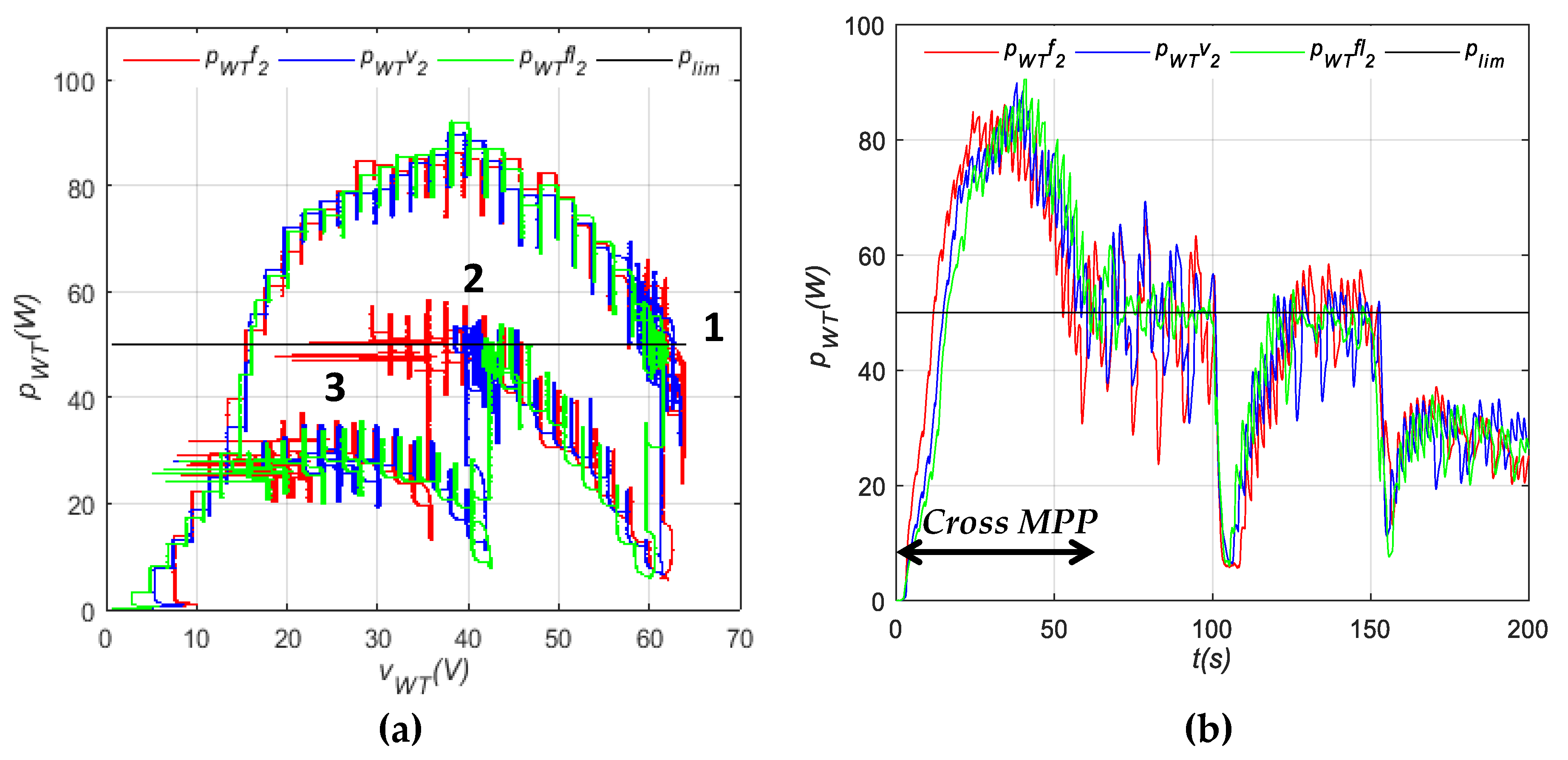
The sudden change of wind speed represents the most critical situation for the wind system stability. Despite the variation of wind speed, the must reach the recommended by the user. A wind speed profile varying from 6.5, 5.5 to 4.5 m/s and a limited power of 50 W are selected (Figure 18). Based on different tests performed to characterize the WT for the selected wind speeds, a presentation of - and - t curves are illustrated in Figure 19. As can be clearly observed, all proposed power control strategies have an identical behavior during wind speed variation. At the start, the wind speed is 6.5 m/s and the system is following the of 50 W which is situated at point 1 with a voltage of 63 V. With the weather’s variation, the wind speed drops to 5.5 m/s, but the is maintained at 50 W. Indeed, prior to reach point 2, the power decreases to 12 W and is then raised to reach the . In this case, the WT is still able to deliver that power since ∈ - curve. Later on, the wind speed drops to 4.5 m/s and, thus, the power drops to 20 W. Since the has become higher than the maximum power that can be generated for this wind speed, the system is unable to deliver it. In such case, the algorithms of the proposed power control strategies are adapted to avoid the drop in power to 0 W if the cannot be reached. Therefore, as can be seen in Figure 19a, when the is not found, the system searches for the MPP (point 3) delivered under this wind speed. In addition, it is also important to notice that the time required to make the transition to the new operating point is almost similar for all proposed power control strategies. However, what changes is the oscillations’ state around . Overall, there are very large oscillations around when the wind speed is high, which could be related to the increase in machine vibrations. Furthermore, it is evident that the FL technique allows for getting better performances around even with a sudden change of wind speed compared to the fixed step size and Newton’s methods.
5. Conclusions
In this study, the performances of LPPT control for an SSWT were investigated. Three different LPPT control power strategies for an SSWT were proposed and tested in order to compare their characteristics and study the effect of some sudden variations (i.e., power variation and weather condition change) on their performances. The proposed methods are the fixed step size, Newton’s method and the FL technique. All these methods are based on the P&O principle. The results show that whatever method is used, the system operates correctly, reaches LPPs, and identifies the direction of the next perturbation. However, what changes are the performances of each method. At first, the results differ according to the perturbation step size used. Indeed, for the fixed step size and Newton’s methods, a large step size contributes to a faster dynamic response but excessive steady-state oscillations, which result in a low efficiency. This situation is reversed when the LPPT is running with a smaller step size. Thus, the LPPT with a fixed step size and variable step size based on Newton’s methods should make a satisfactory tradeoff between the dynamics and oscillations. Regarding the FL method, it has better dynamic performances with more steady oscillations compared to the fixed step size and Newton’s methods. In addition, it is also clearly demonstrated that all methods react correctly during a sudden change of power and wind velocity. They change in an identical way in terms of the response time. The FL technique stabilizes quickly compared to the fixed step size and Newton’s methods, both in power increase or decrease and in rapid change of wind velocity. This method is also interesting for the control of an SSWT in a DC MG. Indeed, it will guarantee less fluctuation in the generated power that can be injected into the public grid.
Future work will concern an effective integration of the SSWT in a DC MG with the adaptation of the proposed control strategies to the constraints linked to the management of power flow in this electrical structure.
Author Contributions
F.L. designed the research. J.A. performed the research, analyzed the data and wrote the paper. F.L. reviewed the paper. All authors have read and agreed to the published version of the manuscript.
Funding
This research received no external funding.
Conflicts of Interest
The authors declare no conflict of interest.
References
- Owusu, P.A.; Asumadu-Sarkodie, S. A review of renewable energy sources, sustainability issues and climate change mitigation. Cogent Eng. 2016, 3, 1–14. [Google Scholar] [CrossRef]
- Fathabadi, H. Novel high efficient speed sensorless controller for maximum power extraction from wind energy conversion systems. Energy Convers. Manag. 2016, 123, 392–401. [Google Scholar] [CrossRef]
- Sechilariu, M.; Wang, B.C.; Locment, F.; Jouglet, A. DC microgrid power flow optimization by multi-layer supervision control. Design and experimental validation. Energy Convers. Manag. 2014. [Google Scholar] [CrossRef]
- Dragicevic, T.; Lu, X.; Vasquez, J.C.; Guerrero, J.M. DC Microgrids-Part I: A Review of Control Strategies and Stabilization Techniques. IEEE Trans. Power Electron. 2016, 31, 4876–4891. [Google Scholar] [CrossRef] [Green Version]
- Al-Ghossini, H.; Locment, F.; Sechilariu, M.; Gagneur, L.; Forgez, C. Adaptive-tuning of extended Kalman filter used for small scale wind generator control. Renew. Energy 2016. [Google Scholar] [CrossRef]
- Hussain, J.; Mishra, M.K. Adaptive Maximum Power Point Tracking Control Algorithm for Wind Energy Conversion Systems. IEEE Trans. Energy Convers. 2016, 31, 697–705. [Google Scholar] [CrossRef]
- Daili, Y.; Gaubert, J.P.; Rahmani, L. New control strategy for fast-efficient maximum power point tracking without mechanical sensors applied to small wind energy conversion system. J. Renew. Sustain. Energy 2015, 7. [Google Scholar] [CrossRef]
- Liu, H.; Locment, F.; Sechilariu, M. Integrated control for small power wind generator. Energies 2018, 11, 1217. [Google Scholar] [CrossRef] [Green Version]
- Orlando, N.A.; Liserre, M.; Mastromauro, R.A.; Dell’Aquila, A. A survey of control issues in pmsg-based small wind-turbine systems. IEEE Trans. Ind. Inform. 2013, 9, 1211–1221. [Google Scholar] [CrossRef]
- Daili, Y.; Gaubert, J.P.; Rahmani, L. Implementation of a new maximum power point tracking control strategy for small wind energy conversion systems without mechanical sensors. Energy Convers. Manag. 2015, 97, 298–306. [Google Scholar] [CrossRef]
- Syahputra, R.; Soesanti, I. Performance improvement for small-scale wind turbine system based on maximum power point tracking control. Energies 2019, 12, 3938. [Google Scholar] [CrossRef] [Green Version]
- Vijay Babu, A.R.; Suresh, K.; Umamaheswara Rao, C.; Saida Reddy, C. Design and implementation of high gain power converter for wind energy conversion system. J. Adv. Res. Dyn. Control Syst. 2018, 10, 307–317. [Google Scholar]
- Liu, H.; Locment, F.; Sechilariu, M. Maximum Power Point Tracking Method for Small Scale Wind Generator Experimental validation. In Proceedings of the 54th Annual Conference of the Society of Instrument and Control Engineers of Japan (SICE), Hangzhou, China, 28–30 July 2015; pp. 87–101. [Google Scholar] [CrossRef] [Green Version]
- Kumar, D.; Chatterjee, K. A review of conventional and advanced MPPT algorithms for wind energy systems. Renew. Sustain. Energy Rev. 2016, 55, 957–970. [Google Scholar] [CrossRef]
- Amir, A.; Amir, A.; Selvaraj, J.; Rahim, N.A. Study of the MPP tracking algorithms: Focusing the numerical method techniques. Renew. Sustain. Energy Rev. 2016, 62, 350–371. [Google Scholar] [CrossRef]
- Nasiri, M.; Milimonfared, J.; Fathi, S.H. Modeling, analysis and comparison of TSR and OTC methods for MPPT and power smoothing in permanent magnet synchronous generator-based wind turbines. Energy Convers. Manag. 2014, 86, 892–900. [Google Scholar] [CrossRef]
- Tiwari, R.; Babu, N.R. Fuzzy logic based MPPT for permanent magnet synchronous generator in wind energy conversion system. IFAC-PapersOnLine 2016, 49, 462–467. [Google Scholar] [CrossRef]
- Urtasun, A.; Sanchis, P.; Marroyo, L. Limiting the power generated by a photovoltaic system. In Proceedings of the 10th International Multi-Conferences on Systems, Signals & Devices 2013 (SSD13), Hammamet, Tunisia, 18–21 March 2013; pp. 1–6. [Google Scholar] [CrossRef]
- Rezk, H.; Eltamaly, A.M. A comprehensive comparison of different MPPT techniques for photovoltaic systems. Sol. Energy 2015, 112, 1–11. [Google Scholar] [CrossRef]
- Belmokhtar, K.; Doumbia, M.L.; Agbossou, K. Novel fuzzy logic based sensorless maximum power point tracking strategy for wind turbine systems driven DFIG (doubly-fed induction generator). Energy 2014, 76, 679–693. [Google Scholar] [CrossRef]
- Meghni, B.; Dib, D.; Azar, A.T. A second-order sliding mode and fuzzy logic control to optimal energy management in wind turbine with battery storage. Neural Comput. Appl. 2017, 28, 1417–1434. [Google Scholar] [CrossRef]
- Calabrese, D.; Tricarico, G.; Brescia, E.; Cascella, G.L.; Monopoli, V.G.; Cupertino, F. Variable structure control of a small ducted wind turbine in the whole wind speed range using a luenberger observer. Energies 2020, 13, 4647. [Google Scholar] [CrossRef]
- Lin, C.-H. Wind Turbine Driving a PM Synchronous Generator Using Novel Recurrent Chebyshev Neural Network Control with the Ideal Learning Rate. Energies 2016, 9, 441. [Google Scholar] [CrossRef] [Green Version]
- Zhang, Y.; Zhang, L.; Liu, Y. Implementation of maximum power point tracking based on variable speed forecasting for wind energy systems. Processes 2019, 7, 158. [Google Scholar] [CrossRef] [Green Version]
- Liu, C.H.; Hsu, Y.Y. Effect of rotor excitation voltage on steady-state stability and maximum output power of a doubly fed induction generator. IEEE Trans. Ind. Electron. 2011, 58, 1096–1109. [Google Scholar] [CrossRef]
- Belhadji, L.; Bacha, S.; Munteanu, I.; Rumeau, A.; Roye, D. Adaptive MPPT applied to variable-speed microhydropower plant. IEEE Trans. Energy Convers. 2013, 28, 34–43. [Google Scholar] [CrossRef]
- Harrag, A.; Messalti, S. Variable step size modified P&O MPPT algorithm using GA-based hybrid offline/online PID controller. Renew. Sustain. Energy Rev. 2015, 49, 1247–1260. [Google Scholar] [CrossRef]
- Messalti, S.; Harrag, A.; Loukriz, A. A new variable step size neural networks MPPT controller: Review, simulation and hardware implementation. Renew. Sustain. Energy Rev. 2017, 68, 221–233. [Google Scholar] [CrossRef]
- Hui, J.C.Y.; Bakhshai, A.; Jain, P.K. An Energy Management Scheme with Power Limit Capability and an Adaptive Maximum Power Point Tracking for Small Standalone PMSG Wind Energy Systems. IEEE Trans. Power Electron. 2016, 31, 4861–4875. [Google Scholar] [CrossRef]
- Bai, W.; Sechilariu, M. DC Microgrid System Modeling and Simulation Based on a Specific Algorithm for Grid-Connected and Islanded Modes with Real-Time Demand-Side Management Optimization. Appl. Sci. 2020, 10, 2544. [Google Scholar] [CrossRef] [Green Version]
- Tiang, T.L.; Ishak, D. Novel MPPT Control in Permanent Magnet Synchronous Generator System for Battery Energy Storage. Appl. Mech. Mater. 2011, 110–116, 5179–5183. [Google Scholar] [CrossRef]
- Papadopoulos, T.; Tatakis, E.; Koukoulis, E. Improved active and reactive control of a small wind turbine system connected to the grid. Resources 2019, 8, 54. [Google Scholar] [CrossRef] [Green Version]
- Kesraoui, M.; Korichi, N.; Belkadi, A. Maximum power point tracker of wind energy conversion system. Renew. Energy 2011, 36, 2655–2662. [Google Scholar] [CrossRef]
- Lazarov, V.; Roye, D.; Spirov, D.; Zarkov, Z. Study of control strategies for variable speed wind turbine under limited power conditions. In Proceedings of the 14th International Power Electronics and Motion Control Conference EPE-PEMC 2010, Ohrid, North Macedonia, 6–8 September 2010; pp. 125–130. [Google Scholar] [CrossRef]
- Linus, R.M.; Damodharan, P. Maximum power point tracking method using a modified perturb and observe algorithm for grid connected wind energy conversion systems. IET Renew. Power Gener. 2015, 9, 682–689. [Google Scholar] [CrossRef]
- Vijayakumar, K.; Kumaresan, N.; Ammasaigounden, N. Speed sensor-less maximum power point tracking and constant output power operation of wind-driven wound rotor induction generators. IET Power Electron. 2015, 8, 33–46. [Google Scholar] [CrossRef]
Figure 1.
The microgrid (MG) overview.

Figure 2.
(a) Wind tunnel; (b) pressure transmitters and Pitot tube.

Figure 3.
Electrical scheme and components of the studied small wind energy conversion system (SWECS).
Figure 3.
Electrical scheme and components of the studied small wind energy conversion system (SWECS).
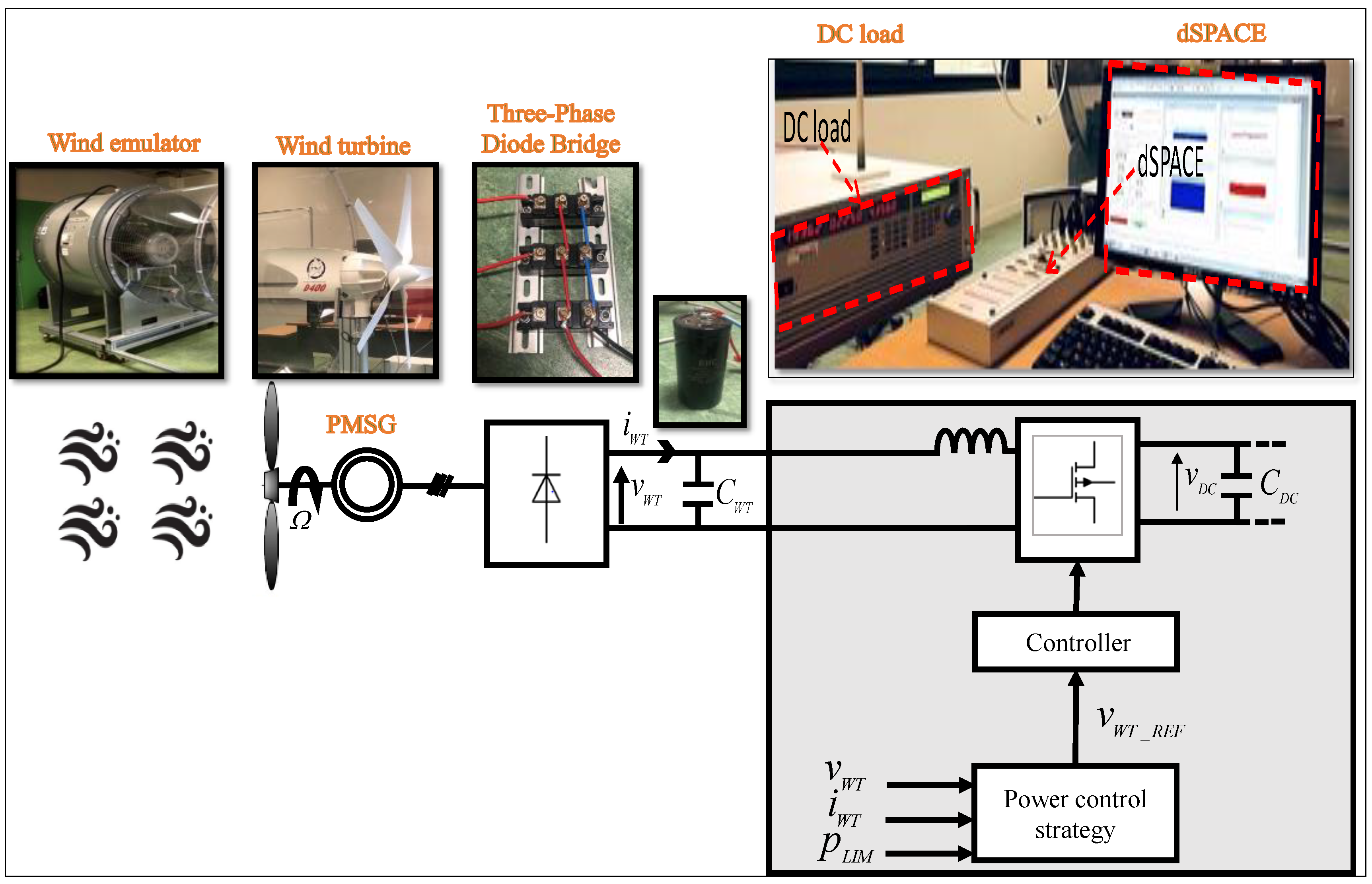
Figure 4.
(a) Electrical power based on the bus voltage ; (b) electrical power based on the bus current ; (c) electrical power based on mechanical speed .
Figure 4.
(a) Electrical power based on the bus voltage ; (b) electrical power based on the bus current ; (c) electrical power based on mechanical speed .
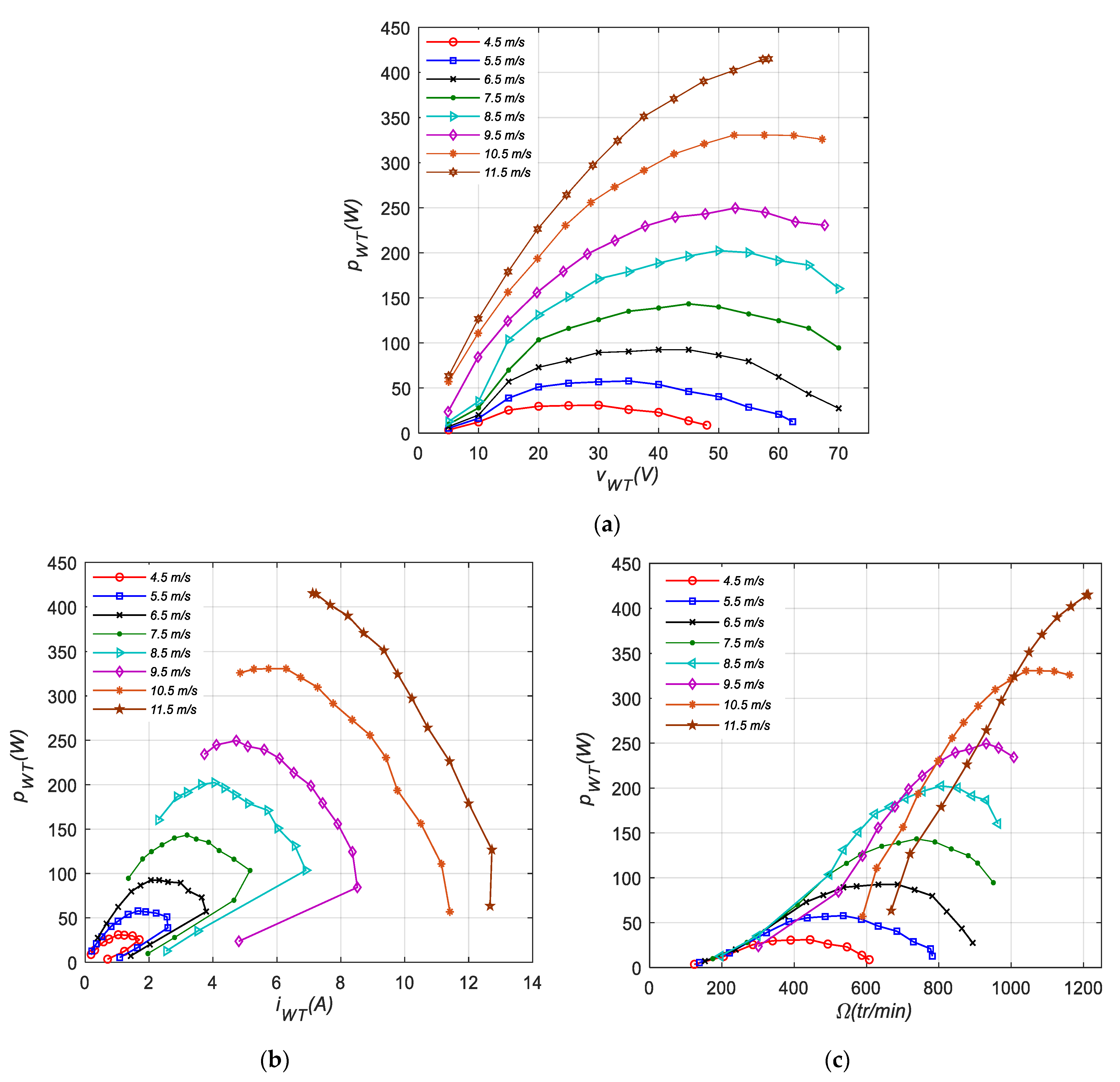
Figure 5.
Operating cases for (a) limited power point 1 (LPP1); (b) LPP2.
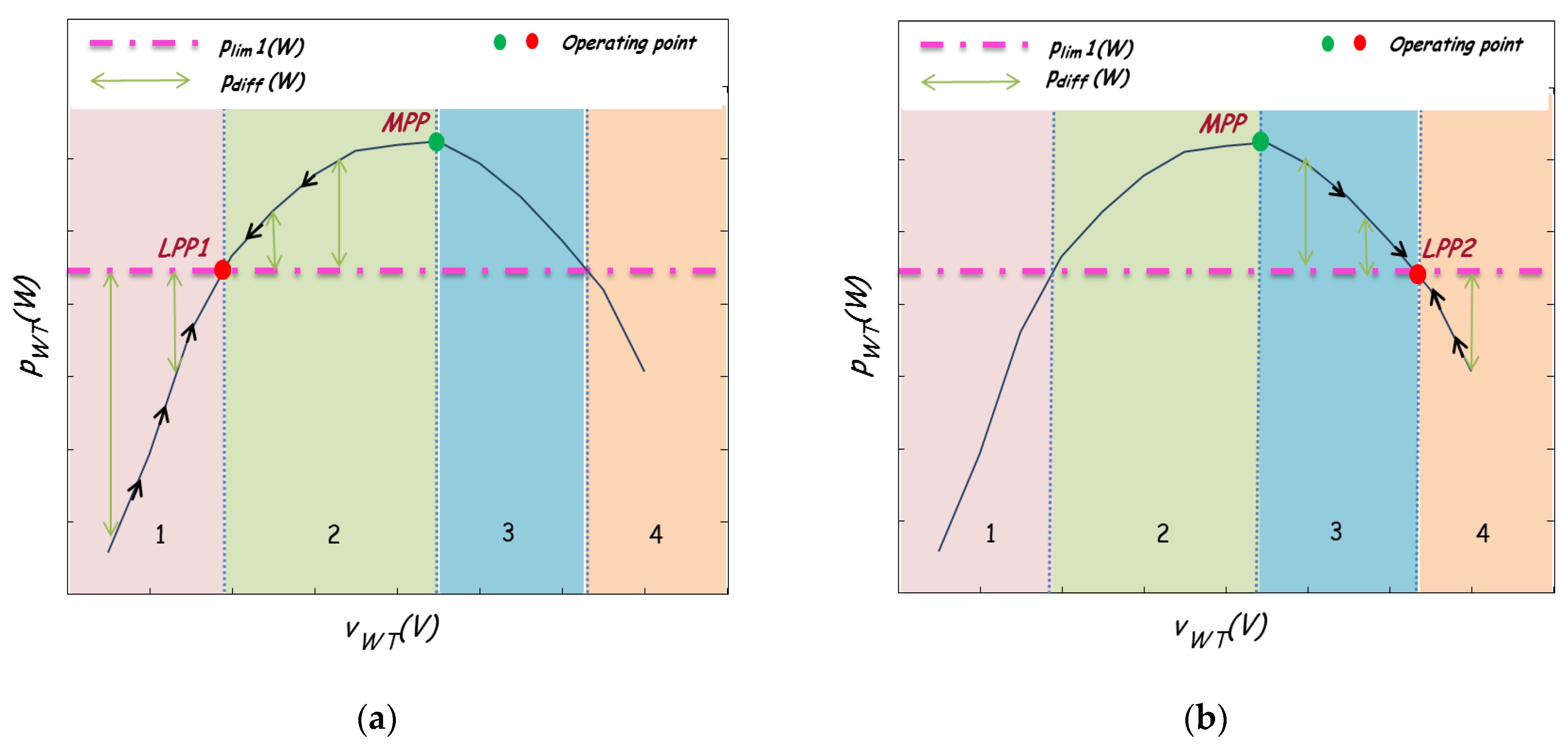
Figure 6.
Principle of perturb and observe (P&O) method for limited power point tracking (LPPT) mode.
Figure 6.
Principle of perturb and observe (P&O) method for limited power point tracking (LPPT) mode.
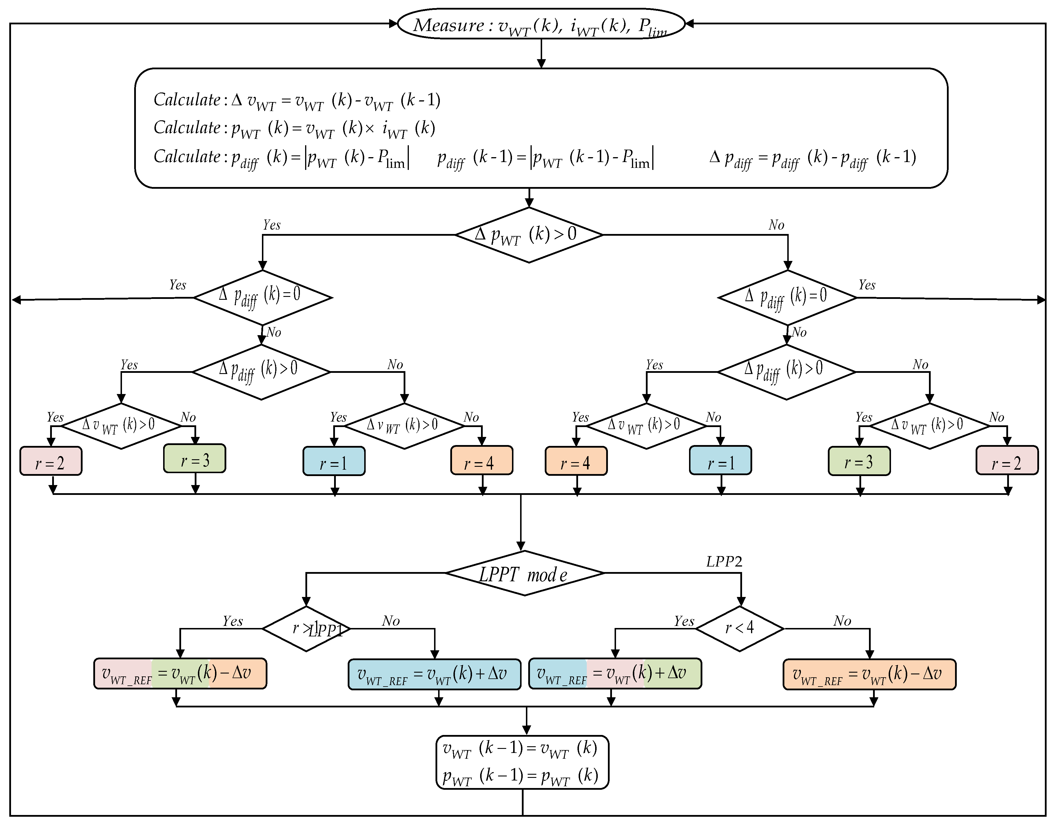
Figure 7.
Structure of fuzzy logic (FL) controller.
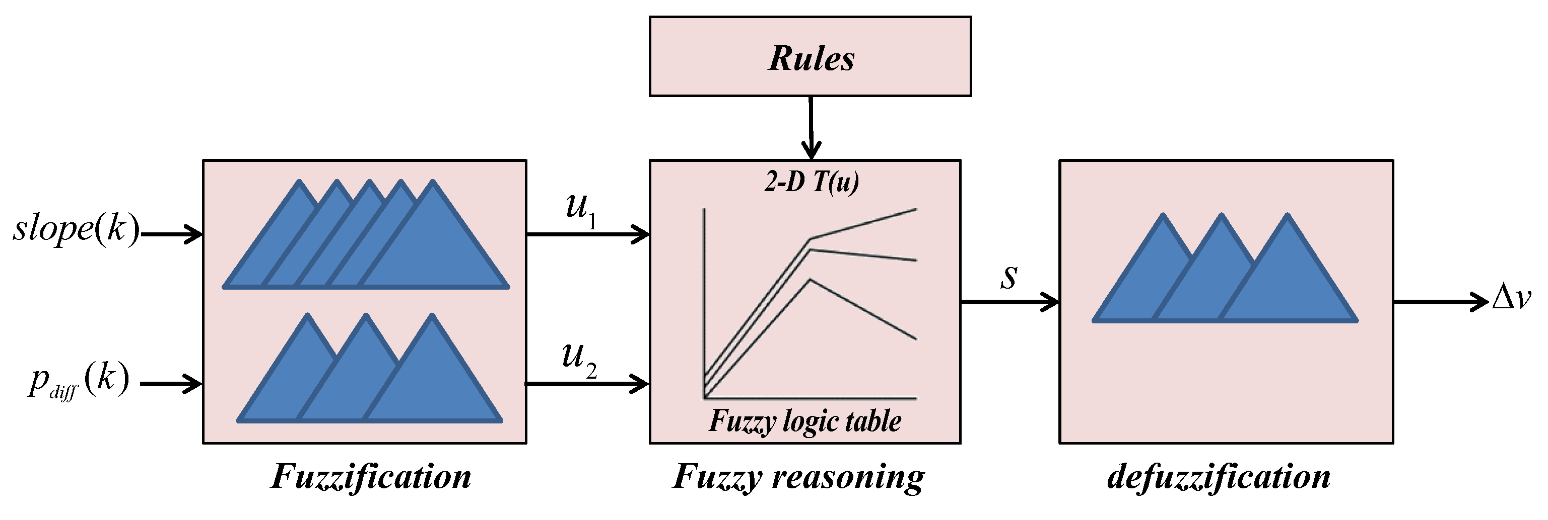
Figure 8.
based on for selected wind speed.

Figure 9.
Fixed step-size P&O for LPP1: (a) evolution of step size ; (b) evolution of ; (c) evolution of ; (d) evolution of .
Figure 9.
Fixed step-size P&O for LPP1: (a) evolution of step size ; (b) evolution of ; (c) evolution of ; (d) evolution of .
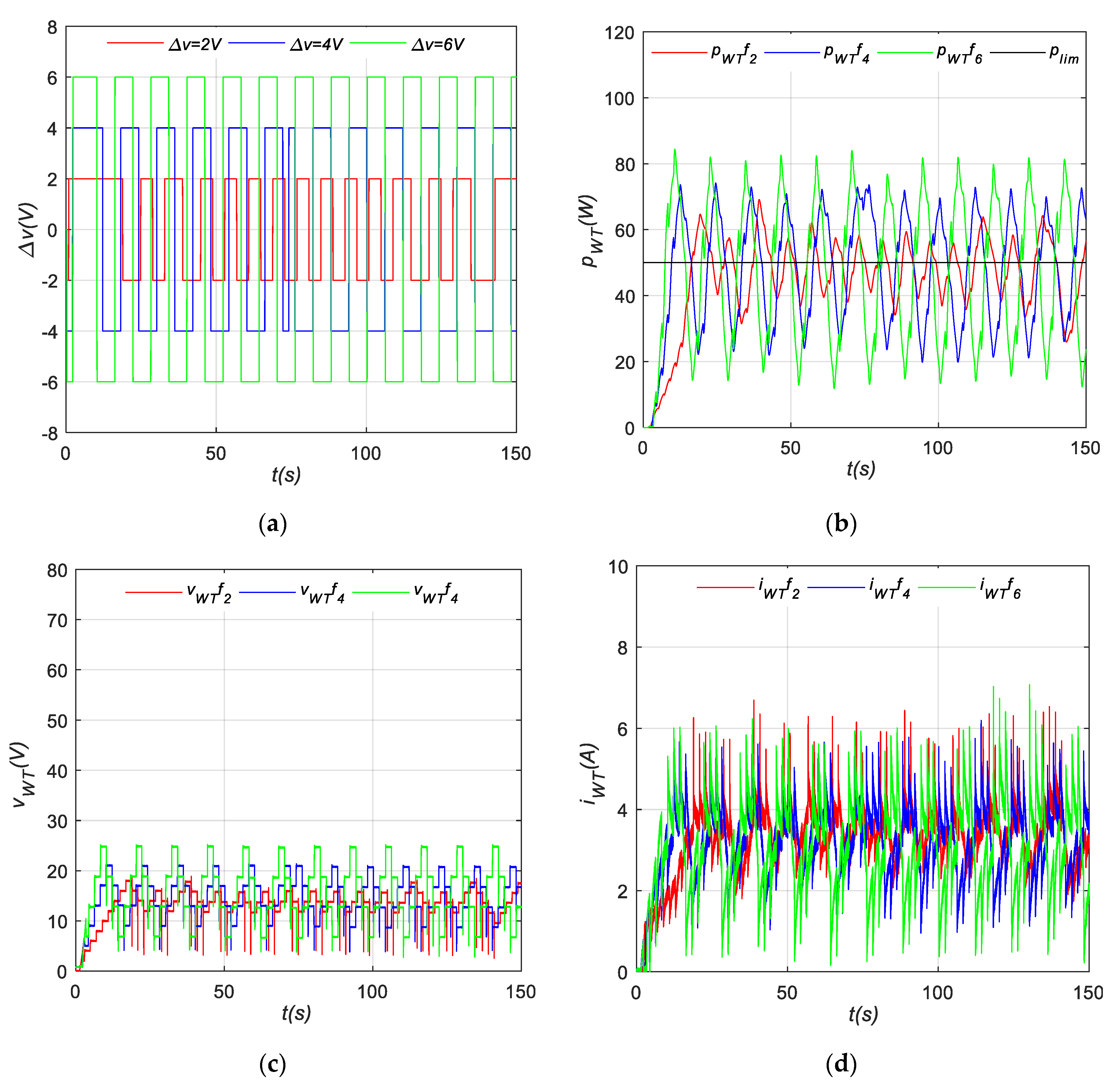
Figure 10.
Fixed step-size P&O for LPP2: (a) evolution of ; (b) evolution of ; (c) evolution of ; (d) evolution of .
Figure 10.
Fixed step-size P&O for LPP2: (a) evolution of ; (b) evolution of ; (c) evolution of ; (d) evolution of .

Figure 11.
Newton’s variable step-size P&O for LPP1: (a) evolution of ; (b) evolution of ; (c) evolution of ; (d) evolution of .
Figure 11.
Newton’s variable step-size P&O for LPP1: (a) evolution of ; (b) evolution of ; (c) evolution of ; (d) evolution of .
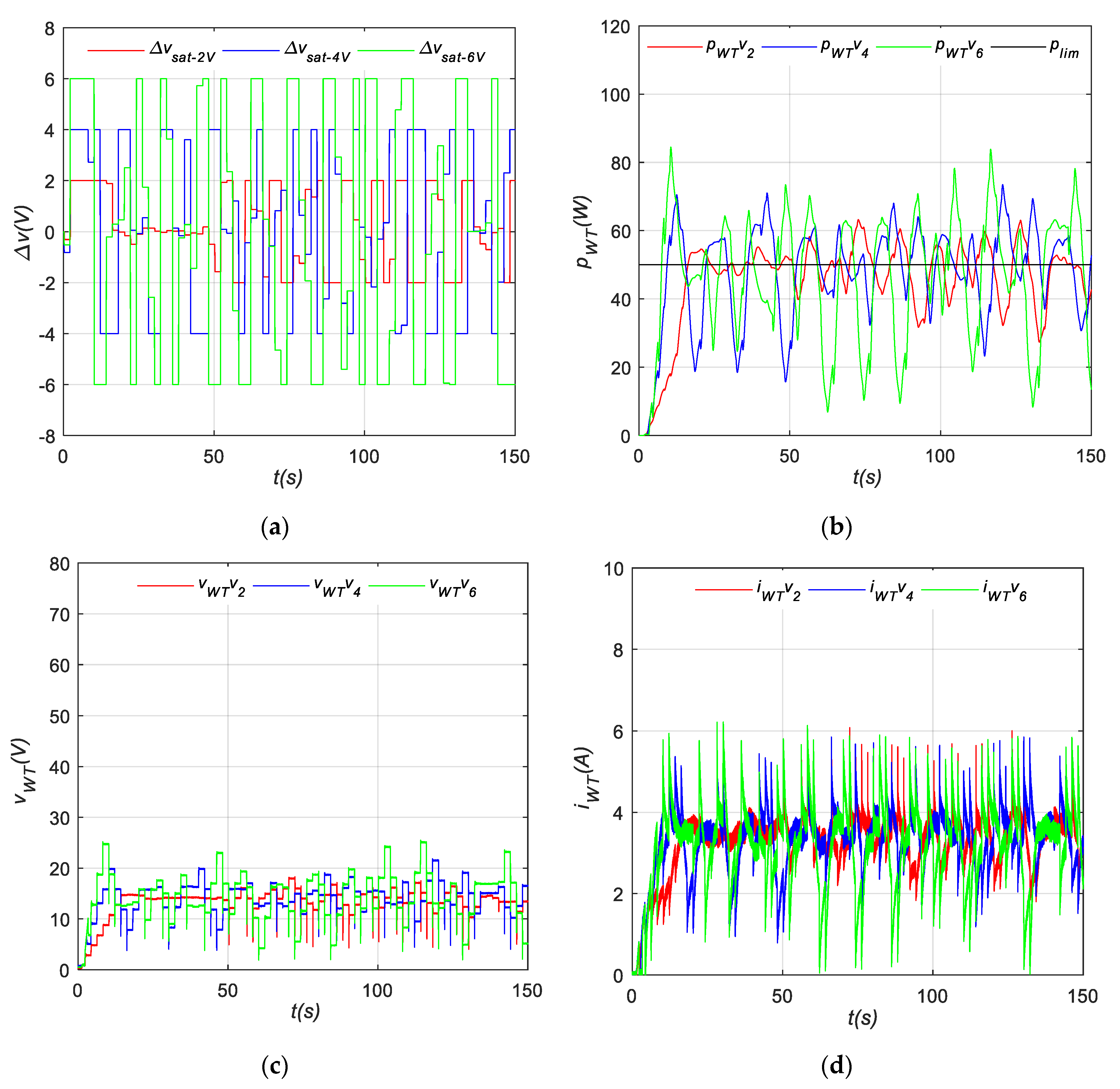
Figure 12.
Newton’s variable step-size P&O for LPP2: (a) evolution of ; (b) evolution of ; (c) evolution of ; (d) evolution of .
Figure 12.
Newton’s variable step-size P&O for LPP2: (a) evolution of ; (b) evolution of ; (c) evolution of ; (d) evolution of .
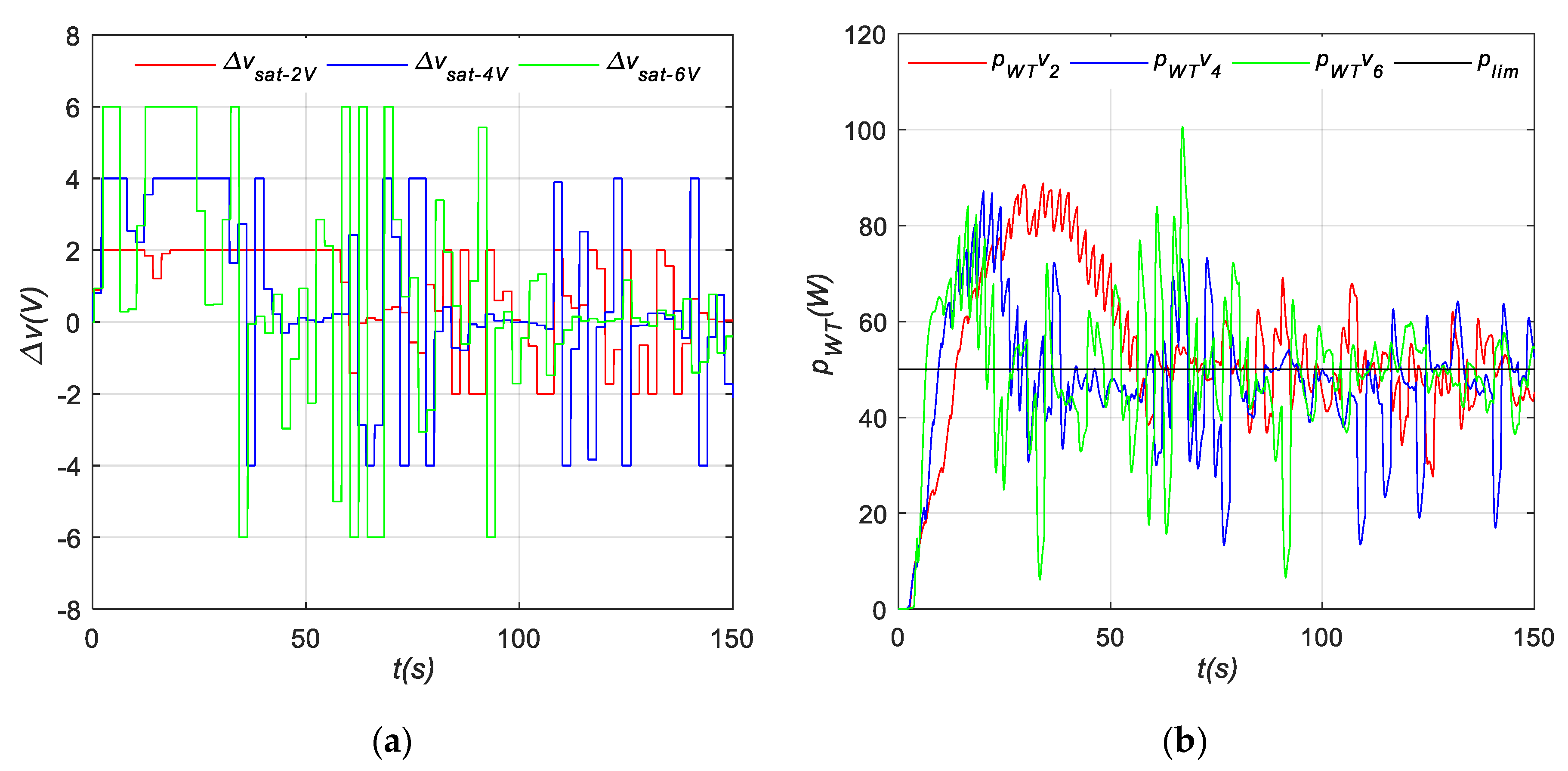

Figure 13.
FL variable step-size P&O for LPP1: (a) evolution of ; (b) evolution of ; (c) evolution of ; (d) evolution of .
Figure 13.
FL variable step-size P&O for LPP1: (a) evolution of ; (b) evolution of ; (c) evolution of ; (d) evolution of .

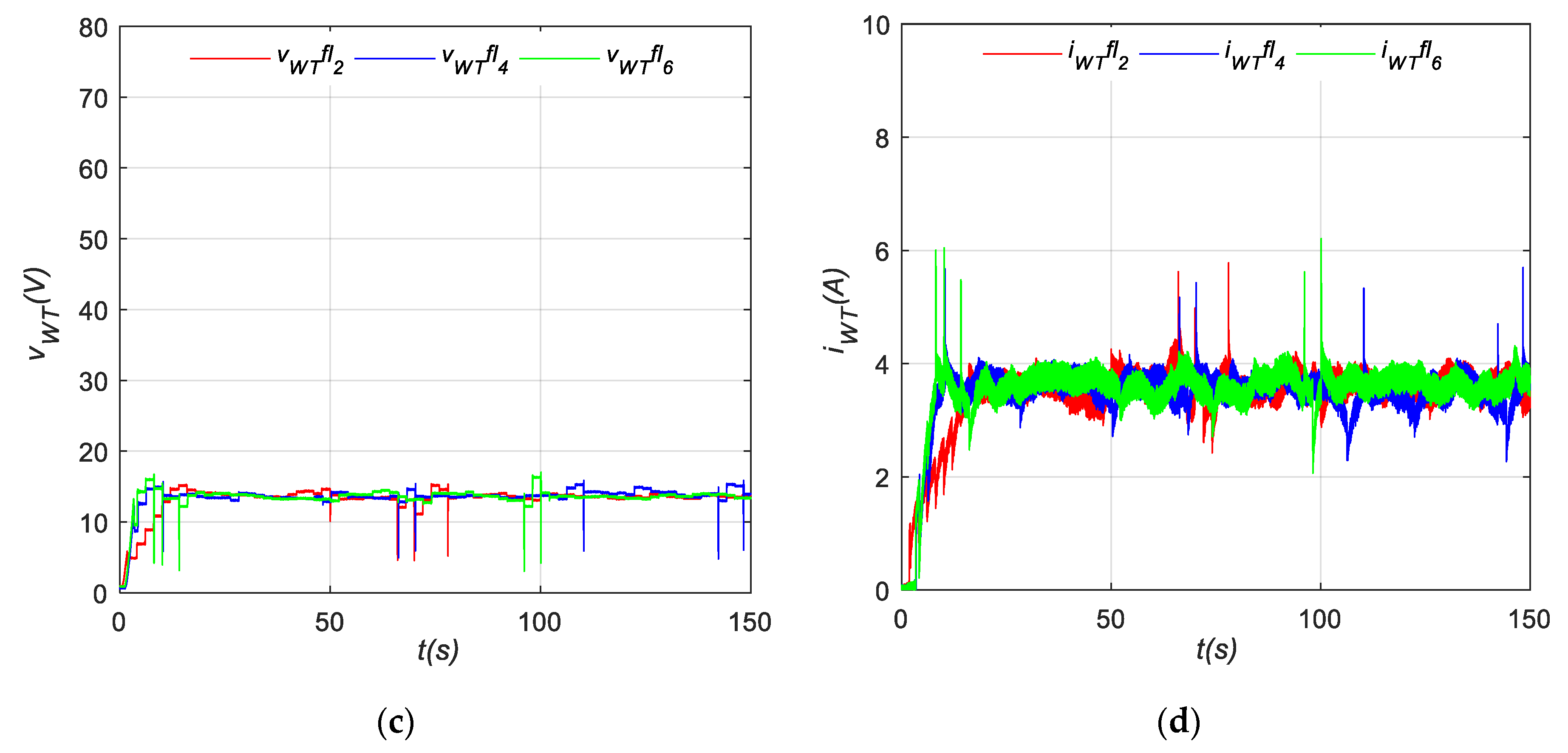
Figure 14.
FL variable step-size P&O for LPP2: (a) evolution of ; (b) evolution of ; (c) evolution of ; (d) evolution of .
Figure 14.
FL variable step-size P&O for LPP2: (a) evolution of ; (b) evolution of ; (c) evolution of ; (d) evolution of .
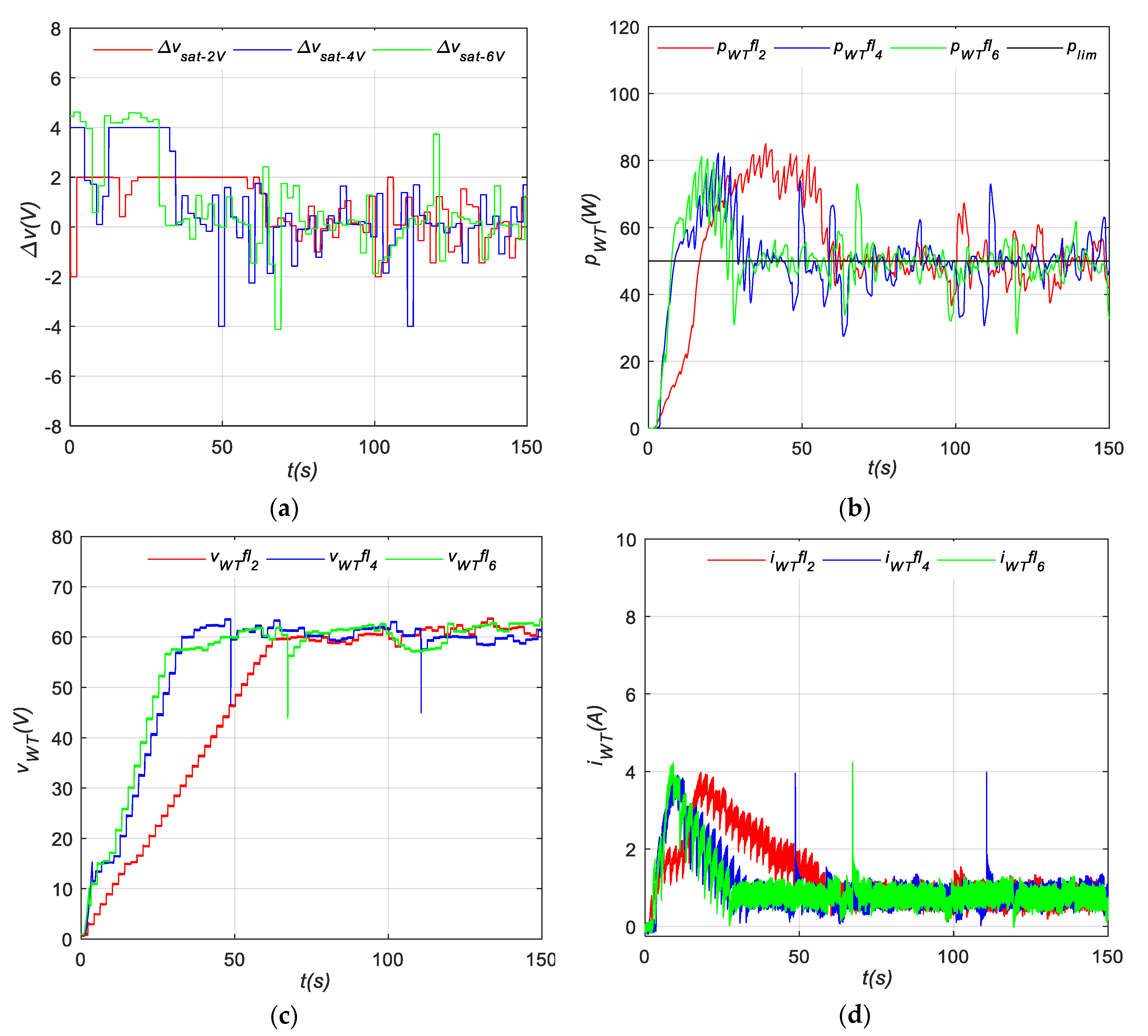
Figure 15.
Comparison of experimental results: (a) evolution of at LPP1; (b) evolution of at LPP2.
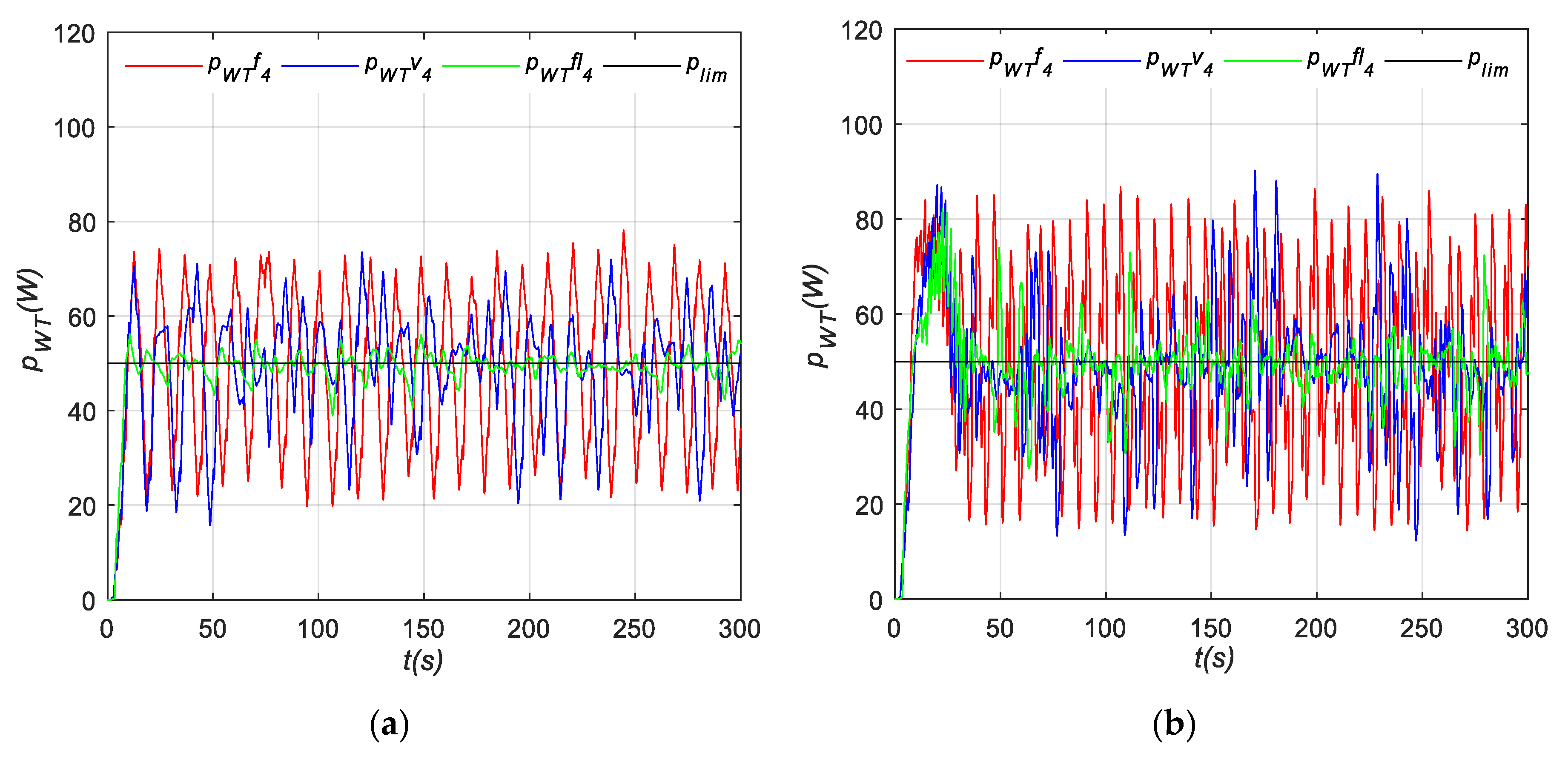
Figure 16.
Statistical analysis of experimental results: (a) evolution of at LPP1; (b) evolution of at LPP2.
Figure 16.
Statistical analysis of experimental results: (a) evolution of at LPP1; (b) evolution of at LPP2.

Figure 17.
Drop in power: (a) sudden increase of ; (b) sudden decrease in .
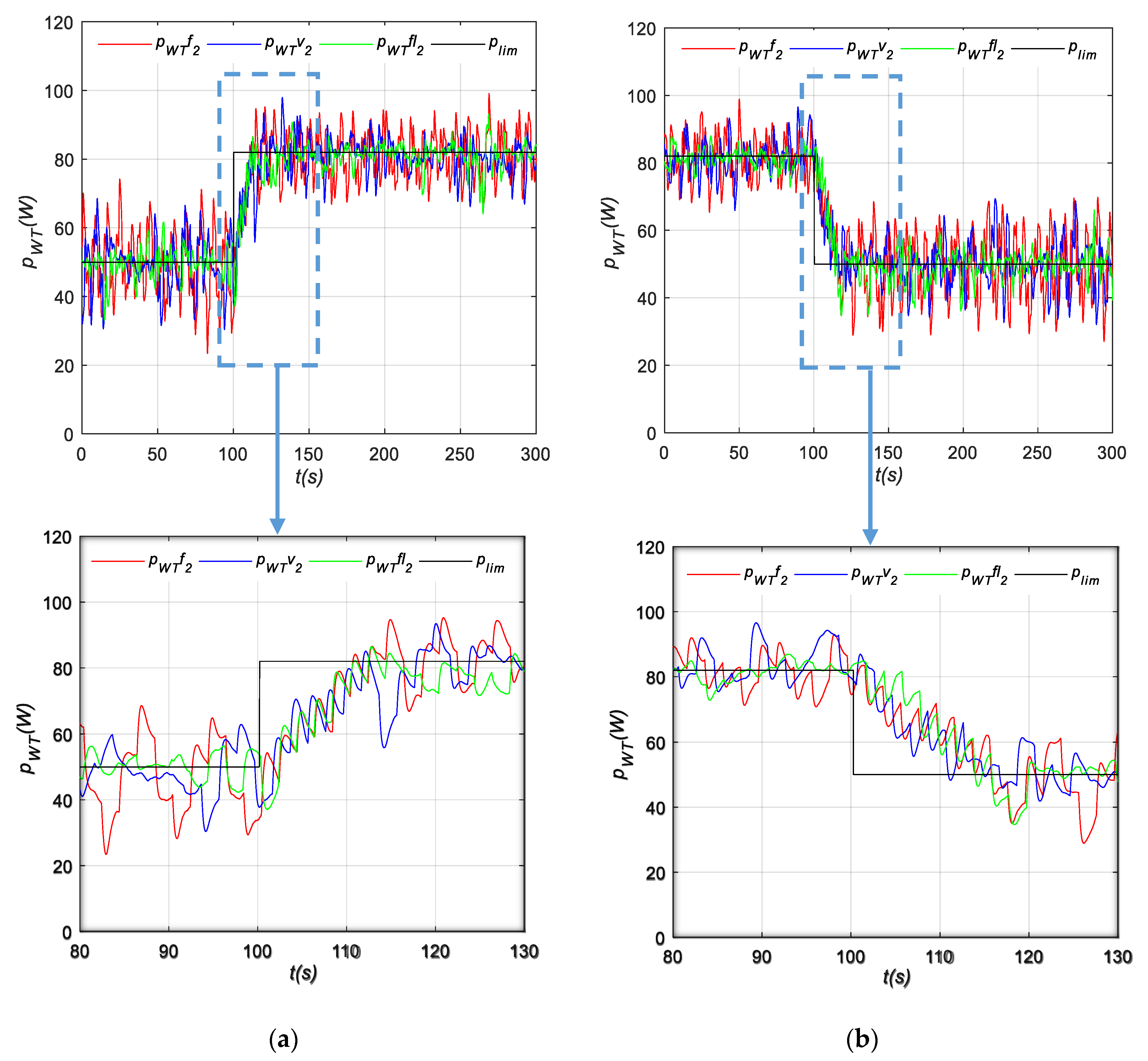
Figure 18.
Wind velocity profile.
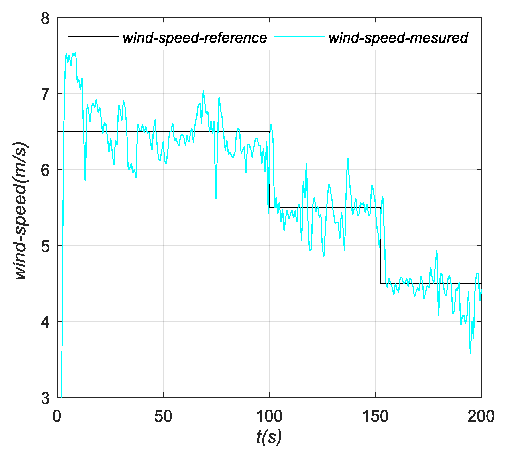
Figure 19.
Drop in wind velocity: (a) based on ; (b) evolution of in time.

Table 1.
Rule base for LPPT mode. (N: negative; P: positive; Z: zero; S: small; B: big)
| N | Z | P | ||
|---|---|---|---|---|
| NB | z | z | z | |
| NS | p | z | n | |
| ZE | p | z | n | |
| PS | p | z | n | |
| PB | z | z | z | |
Table 2.
reached using different control method strategies. SD: standard deviation.
| Control Strategy Method | LPP1 (Mean ± SD) | LPP2 (Mean ± SD) |
|---|---|---|
| Fix step size | 48.6 ± 15.4 | 49.8 ± 19.3 |
| Newton’s method | 49.5 ± 10.0 | 48.3 ± 12.7 |
| Fuzzy logic | 49.6 ± 2.4 | 49.3 ± 5.6 |
Publisher’s Note: MDPI stays neutral with regard to jurisdictional claims in published maps and institutional affiliations. |
© 2020 by the authors. Licensee MDPI, Basel, Switzerland. This article is an open access article distributed under the terms and conditions of the Creative Commons Attribution (CC BY) license (http://creativecommons.org/licenses/by/4.0/).
Share and Cite
MDPI and ACS Style
Aourir, J.; Locment, F. Limited Power Point Tracking for a Small-Scale Wind Turbine Intended to Be Integrated in a DC Microgrid. Appl. Sci. 2020, 10, 8030. https://doi.org/10.3390/app10228030
AMA Style
Aourir J, Locment F. Limited Power Point Tracking for a Small-Scale Wind Turbine Intended to Be Integrated in a DC Microgrid. Applied Sciences. 2020; 10(22):8030. https://doi.org/10.3390/app10228030
Chicago/Turabian StyleAourir, Jamila, and Fabrice Locment. 2020. "Limited Power Point Tracking for a Small-Scale Wind Turbine Intended to Be Integrated in a DC Microgrid" Applied Sciences 10, no. 22: 8030. https://doi.org/10.3390/app10228030
Note that from the first issue of 2016, this journal uses article numbers instead of page numbers. See further details here.