Wind Turbines Optimal Operation at Time Variable Wind Speeds
by
 ,
,
Mihaela-Codruta Ancuti
1,*, 
Sorin Musuroi
1,
Ciprian Sorandaru
1,
Marian Dordescu
2 and
Geza Mihai Erdodi
3 1
Electrical Engineering Department, Faculty of Electrical and Power Engineering, University Politehnica Timisoara, 300223 Timisoara, Romania
2
Department of Engineering Sciences in the Electrical Field, Constanta Maritime University, 900663 Constanta, Romania
3
Department of Automation, Industrial Engineering, Textiles and Transport, Aurel Vlaicu University of Arad, 310130 Arad, Romania
*
Author to whom correspondence should be addressed.
Appl. Sci. 2020, 10(12), 4232; https://doi.org/10.3390/app10124232
Submission received: 30 April 2020
/
Revised: 7 June 2020
/
Accepted: 16 June 2020
/
Published: 20 June 2020
(This article belongs to the Special Issue Wind Turbine Data, Analysis and Models)
Abstract
:The wind turbine’s operation is affected by the wind speed variations, which cannot be followed by the wind turbine due to the large moment of the power plant’s inertia. The method proposed in this paper belongs to the wind turbine power curves (WTPC) approach, which expresses the power curve of the permanent magnet synchronous generator (PMSG) by a set of mathematical equations. The WTPC research papers published before now have not taken into consideration the total power plant inertia at time-variable wind speeds, when the wind turbine’s optimal operation is very difficult to be reached, and its efficiency is thus threatened. The study is based on a wind turbine having a large moment of total inertia, and demonstrates, through extensive simulation results, that the optimal values of the PMSG’s power can be determined based on the kinetic motion equation. This PMSG’s optimal power represents an ideal time-varying curve, and the wind turbine should be controlled so as to closely follow it. For this purpose, proportional integral (PI) and proportional integral derivative (PID) type-based control methods were implemented and analyzed, so that the PMSG’s power oscillations could be reduced, and the PMSG’s angular speed value made comparable to the optimal one, meaning that the wind turbine operates within the optimal operation area, and is efficient. The simulations are actually the numerical solutions obtained by using the Scientific Workplace simulation environment, and they are based on the wind speed measurements collected from a wind farm located in Dobrogea, Romania.

1. Introduction
Renewable energy has become a very important research area during the last few decades, and wind farms are a resource-efficient option for generating electric energy. The main drawback, though, is that the wind resources are affected by wind volatility, and furthermore, sudden wind speed variations lead to the unstable operation of the wind turbine [1].
As is highlighted in [2], from the energy point of view, the operation of the wind turbines within the optimal area was treated mainly for constant wind speeds over time. In reality, the wind speed is a time-varying function, and in order to operate within the optimal area from the energy point of view, the angular speed of the permanent magnet synchronous generator (PMSG) must follow the wind speed variation in time, because the PMSG’s optimal angular speed is directly proportional to the wind speed value, as was shown in [3].
Tracking the maximum power point (MPP) is the essence of the variable speed wind turbines’ control, since it determines their efficiency. The MPP is achieved by always adapting the wind turbine’s speed to the wind speed [4].
There are five main categories of MPP tracking methods: power signal feedback (PSF) control [5], optimal torque (OT) control [6], tip-speed ratio (TSR) control [7] and perturbation and observation (P&O) control [8,9]. There are also artificial intelligence techniques, such as fuzzy logic [10], artificial neural networks [11], intelligent search algorithms [12] and wind turbine power curves (WTPC) [13,14,15].
PSF- and OT-based MPP tracking methods employ the generator’s exact model, commonly used in large-scale wind turbines [6,7]. The torque is usually estimated using the Kalman filter [16].
Since the wind turbines can change their rotation speed to follow changes in wind speed, this means that for each wind speed there is an ideal rotational speed, which is called the optimal tip-speed ratio (TSR), and is different for each wind turbine [7]. Thus, the TSR-based MPP tracking method uses the wind turbine’s exact model. The wind speed and the tip-speed ratio are estimated using the Newton–Raphson method. The error between the estimated torque and the steady optimal torque is used as the feed-forward signal to control the generator torque. Unfortunately, there is a conflict between the rapid wind variations and the slow dynamic response of the wind turbines, due to the large inertia of the generator.
Regarding the P&O method, it was demonstrated in the literature that this fails to follow the MPP trajectory of the under rapid wind variations [8].
For high efficiency, instantaneous MPP is highly demanded, but this claims high controller robustness against parameter variations and external disturbances. Therefore, fuzzy and artificial intelligence-based MPP tracking methods represent a flexible medium, that proposes solutions to problems that cannot be tackled with traditional methods. Many papers have stated that the sliding mode control approach is more robust with respect to parameter variations and external disturbances [17]. Nevertheless, chattering is its main drawback. To address this, higher order sliding mode control was developed [18].
Due to the uncertain nature of the wind, in order to make wind energy a reliable source, accurate models for predicting the delivered power and performance monitoring of wind turbines are needed. The wind turbine’s power curve, which gives the turbine’s delivered power at a specific wind speed, provides a convenient way to model the performance of wind turbines. A number of methods have been proposed in the literature for WTPC modelling, as follows: parametric models, parameter estimation, data preprocessing, evaluation of model, and nonparametric models (i.e., the artificial neural networks method and the fuzzy logic method, this one being used when the data collected from the wind farms is voluminous, and usually contains errors). They have their own advantages and disadvantages. The power curve models based on polynomial approximation are simple to use, but only for small systems [13]. Most of the models are developed from the manufacturer’s curves of wind turbines [14], which are turbine-specific, and they can be applied in the power prediction of single turbines and in sites with steady winds [15]. As the wind turbine’s power is strongly dependent on the wind speed at the wind farm site, the selection of an appropriate wind speed model, along with the power curve model, is the main requirement for accurate prediction of the wind farm’s output. Therefore, improved models are required, which should be able to minimize the prediction errors. In consequence, the method proposed in this paper belongs to the WTPC approach, which express the shape of the PMSG’s power curve by a set of mathematical equations. Determination of the coefficients of these equations requires fitting the data to the mathematical model [13].
Furthermore, all these methods, PSF, OT, TSR, P&O, artificial intelligence techniques and WTPC, at some level fail in the proper detection of the maximum power point. Furthermore, the problems become more complex for time-varying wind speeds, due to the high value inertia moments [19,20].
To cope with these problems, the moment of inertia has to be considered, making it possible to accurately detect the MPP, even under rapid wind variations.
In the literature, there are only a few studies on methods to eliminate the inertial effect at variable wind speeds, when the optimal operation of the wind turbine is very hard to achieve [14]. However, as regards the WTPC method, there is no study taking into account the inertia. Therefore, the method proposed in this paper is based on the mathematical model of the wind turbine, which includes its moment of inertia, too.
The paper is comprised of seven sections. Section 1 presents an overview of the arising problems regarding reaching a good wind turbine efficiency; Section 2 presents the wind turbines’ mathematical model, on which the study is based; Section 3 describes the methodology of determining the PMSG’s optimal power; Section 4 presents the implementation of a proportional integral (PI) type control applied to the PMSG’s optimal power; in Section 5, a proportional integral derivative (PID)-type control is applied to the PMSG’s optimal power; Section 6 presents a case study, and in Section 7, the conclusion is drawn. The case study is based on a real wind turbine’s data, collected from a real wind farm and provided in [21]. The installed wind turbines are of 2.5 (MW) nominal output power, and of the three blades type, are manufactured by General Electric company and have the characteristics presented in Table A1, which can be found in the Appendix paragraph.
Along with the case study presented in this paper, the operation of one wind turbine is analyzed for wind speeds measured with a sampling step of 30 (s). Based on the values of the wind speed, the maximum values of the chosen wind turbine’s power are determined, . Then, the operation of the wind turbine, at MPP, is analyzed, meaning that the optimal values of the PMSG’s power can be determined based on the measured wind speed, so that the PMSG’s angular speed tends towards the PMSG’s optimal angular speed.
Two control methods for constraining the PMSG’s power to follow the optimal one are in this paper analyzed: one based on the PI-type regulator, and the second one based on the PID-type regulator. The values of the regulator coefficients were determined by the trial and error method. Then, finally, the optimal power values of the PMSG are compared to the ones obtained by implementing two types of control, based on either the PI or PID regulators.
The simulations are actually represented by the numerical solutions obtained by using the MAPLE core of the Scientific Workplace simulation environment, and they are based only on the measured wind speed from the experimental data collected from the wind farm.
A list containing the main variables used in this paper is provided by Table A2 in Appendix.
2. Wind Turbine’s Mathematical Model
The study presented in this paper is based on the classical mathematical model of the wind turbine, as given in [3]. It allows for the optimal values of the PMSG’s angular speed, , to be determined, so that the captured wind energy is maximum.
The characteristic of the wind turbine’s power, , which also represents the wind turbine’s mathematical model, has, in general, the below shape
where is the wind speed, is the PMSG’s angular speed, and the parameters are specific to the used wind turbine, and can be determined from the data sheet provided by the wind turbine’s manufacturer.
For time-varying wind speeds, , the wind turbine’s power, , varies between a minimum value and a maximum value, depending on the PMSG’s angular speed value, .
The maximum value of the wind turbine’s power, is obtained from Equation (1), for the PMSG’s optimal angular speed, , by canceling the wind turbine’s power derivative
which yields to
where represents the proportional constant, determined in [3],
Furthermore, the wind turbine’s power is zero for (the maximum value of the PMSG’s angular speed), which, employed in Equation (1), yields to
whose solution is
Combining Equations (3) and (6), the ratio is obtained as
which will be useful in determining the coefficients.
Finally, by replacing Equation (3) in Equation (1), the maximum value of the wind turbine’s power, , is obtained as
where
represents another proportional constant, determined in [3].
3. PMSG’s Optimal Power Determination based on the Kinetic Motion Equation
The kinetic motion equation, as depicted in [2], is as shown below
where is the moment of total inertia, is the PMSG’s angular speed, is the wind turbine’s developed torque, is the PMSG’s developed torque, and all of them are related to the PMSG’s shaft.
Multiplying (10) by , the following expression results
where:
- the first term, which is dependent on the moment of total inertia, is called the “inertial power”,
- the second term, , which is dependent on the PMSG’s angular speed, , and on the wind speed, , as depicted by Equation (1), represents the “wind turbine’s power”.
- the third term, which is dependent on the PMSG’s angular speed, , and on the load resistance, represents the PMSG’s power, .
Therefore, Equation (11) can also be written as
Then, integrating Equation (11), the below relationship can be obtained as
where is the PMSG’s angular speed at time instant , is the PMSG’s angular speed at time instant , is the average power delivered by the wind turbine, and is the PMSG’s average power.
Thus, from Equation (14), the energy balance of the wind turbine was obtained as
where:
- the first term, , represents the wind energy captured by the wind turbine during the time interval, ,
- the second term, , represents the energy delivered by the PMSG to the main grid,
- the third term, , represents the kinetic energy,where the variation of the kinetic energies, , can be determined very precisely by measuring the PMSG’s angular speed, .
Remark 1: The kinetic energy is the useful energy that also includes the PMSG’s efficiency, thus generating the additional electrical power from the PMSG’s terminals.
The average power delivered by the PMSG can be determined from Equation (14) by using the below relationship:
Similar to Equation (19), the optimal values of the PMSG’s power are obtained for the MPP operation when its angular speed, , becomes equal to the PMSG’s optimal angular speed, , which depends linearly on the time-varying wind speed, , as described by Equation (3). Thus, and by employing Equation (3) in Equation (11), the result is that
which, replacing Equation (9) in Equation (20), becomes
where
In conclusion, based on the measured time-varying wind speed values, , the optimal values of the PMSG’s power, can be determined using Equation (21). In essence, this means that the wind turbine operates at the MPP, and thus, the PMSG’s angular speed, , tends towards the optimal value, .
4. PMSG’s Optimal Power Control Based on the PI-type Regulator
The time-varying curve of the PMSG’s optimal power was previously determined based on the kinetic motion equation, and it represents the ideal (theoretical) curve to be followed by the wind turbine in order to operate at the maximum power point. This means that the wind turbine should be controlled in such a way as to closely follow the ideal curve.
Thus, the main objective is to control the PMSG’s power curve, following the PMSG’s optimal power curve (), or, as otherwise stated, the PMSG’s angular speed becomes equal to its optimal speed (). One way of doing this is by implementing a control based on a PI-type regulator.
The equation of the PI-type regulator is below described:
where is the reference value of the PMSG’s power for the case of a PI-type based control, is the computed/measured value of the PMSG’s power, , is the proportional constant and is the integral constant of the PI regulator.
By derivation, Equation (23) becomes
Then, by replacing Equation (3) in Equation (24), it results in
The PMSG’s power in Equation (25), , can be determined from the kinetic motion equation from Equation (11).
Replacing Equation (1) in Equation (11), the below kinetic motion equation is obtained as
The kinetic motion Equation (26), together with the PI-type regulator Equation (25), defines the below system of differential equations used in the simulation environment for determining the PMSG’s power curve and the PMSG’s angular speed:
5. PMSG’s Optimal Power Control Based on the PID-type Regulator
In this paragraph, another control method for ensuring the PMSG’s power follows the PMSG’s optimal power, () or (), is proposed, and consists of implementing a control based on a PID-type regulator.
The equation of the PID-type regulator is
where is the reference value of the PMSG’s power in the case of a PID-type based control, is the computed/measured value of the PMSG’s power, is the proportional constant, is the integral constant and is the derivative constant of the PID regulator.
Derivation of Equation (28) yields to
Then, replacing Equation (3) in Equation (29), it results to
The PMSG’s power in (30), , can be determined from the kinetic motion equation in Equation (21), written as below:
Since, in Equation (30), there is a second order derivative of the time-varying wind speed curve, , the derivation of the kinetic motion equation from Equation (31) is imposed, obtaining
where the following notation has been made: .
The derived kinetic motion Equation (32), together with the PID-type regulator equation in Equation (30), defines the below system of differential equations used in the simulation environment for determining the PMSG’s power curve and the PMSG’s angular speed:
6. Case Study
6.1. PMSG’s Optimal Power Determination
In what follows, the objective is to determine the optimal values of the PMSG’s power , delivered by one of the wind turbines within [21].
Since the depends on , the main input parameter that could be measured is the time-varying wind speed. The wind farm in [21] provided the wind speed measurements, sampled with a step of 30 (s), as shown in the below presented Table 1.
Thus, employing Equation (34) in Equation (7), it results to
Using Equations (35) and (37) in Equation (4), it yields to
Using Equations (36) and (38) in Equation (9), the value of parameter is obtained as
Finally, employing Equations (38) and (39), Equation (1) becomes
Accuracy in finding the PMSG’s optimal power curve can be achieved via the accuracy of the modelled wind speed. Thus, considering a parabolic shape for the approximated wind speed time variation, described as
and using the measurements data from Table 1, the below equations system results:
the solutions of which are
Finally, an approximation for the wind speed time variation is obtained, as depicted below and shown in Figure 1.
The first-order derivative of the wind speed time variation from Equation (44), which is also depicted in Figure 1, can be obtained by using the below equation:
The approximated wind speed reaches a maximum value for the time instant (see Figure 1), obtained by canceling its derivative in Equation (45), , whose solution is (s).
Remark 2: In Figure 1, it can be seen that the approximated wind speed time variation depicted in (44) is very close to the measured wind speed curve, , obtained as depicted in Table 1.
The maximum value of the wind turbine’s power can be determined from Equations (18) and (36), using the below relationship:
which, by replacing with Equation (44), becomes
Following Equations (35) and (36), and replacing the moment of total inertia with the value of , which is known from [21], the PMSG’s optimal power curve, , defined by Equation (21), for a certain wind speed time variation, , can be written as below:
Based on the wind speed time variation, given in Figure 1, it becomes
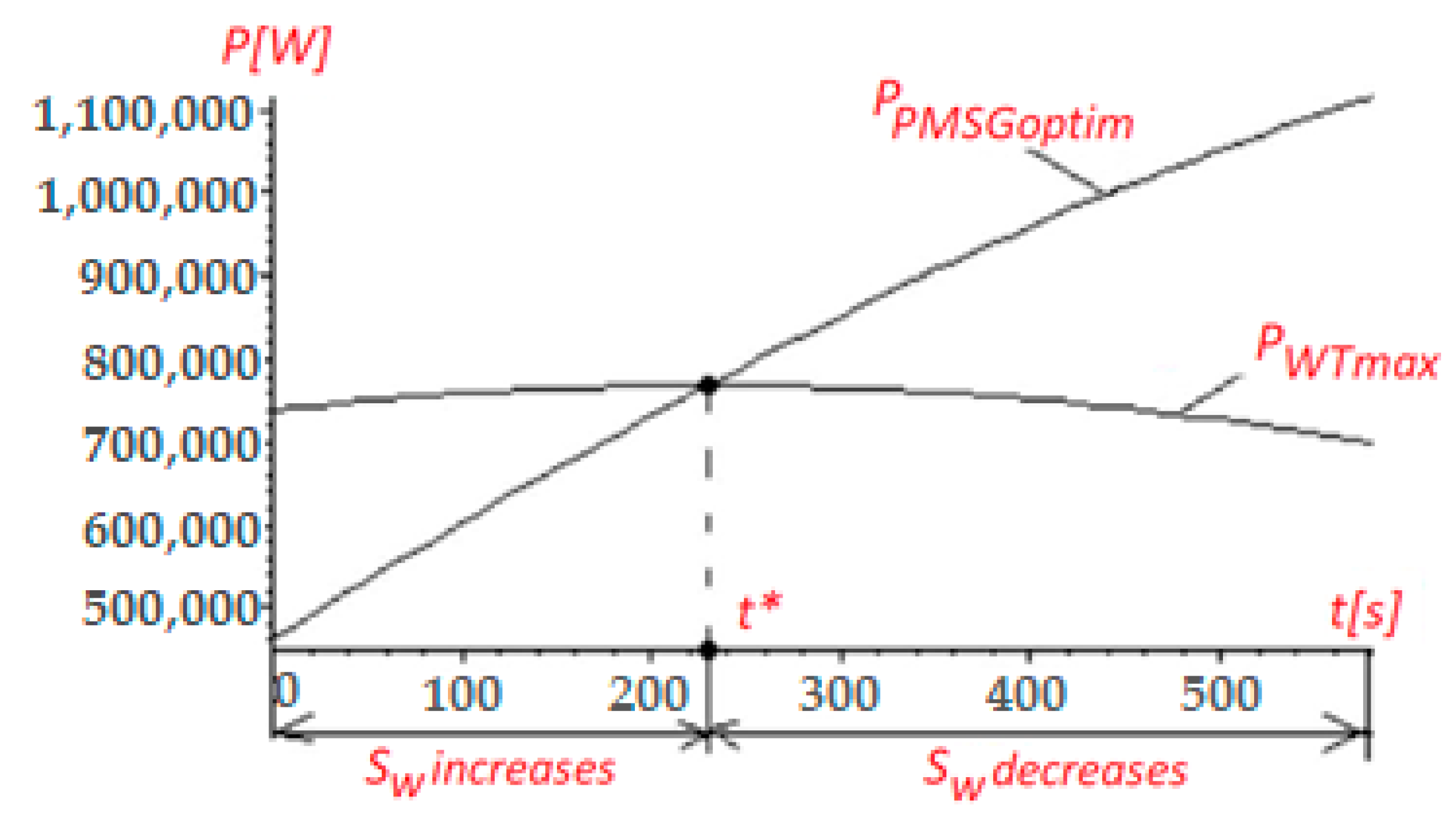
Figure 2 below presents the time variations of the maximum wind turbine’s power and the PMSG’s optimal power.
Integrating the PMSG’s optimal power described by Equation (49), for a time interval from 0 (s) to 570 (s), the value of the energy delivered by the PMSG to the main grid, , is the below:
The maximum value of the captured wind energy,, during the time interval between 0 (s) and 570 (s), is obtained by integrating the wind turbine’s maximum power into (47):
Remark 3: The value of the captured wind energy is less than the value of the delivered energy, the difference between the two values being found in the kinetic energy:
Then, using Equations (50) and (52), Equation (15) becomes
which is equal to from (51).
Thus, the energy balance in Equation (15) is checked.
Remark 4: For high values of the moment of total inertia, , and of the wind speed derivative, , the value of the inertial power, , is comparable with the wind turbine’s power values, , and the PMSG’s optimal power values, . For example, for the time instant, (s) the wind speed derivative in Equation (50) has the below value:
while the power’s values are:
● the inertial power from Equation (22),
● the optimal PMSG’s power from Equation (49),
● the maximum wind turbine’s power from Equation (47),
It can be observed that the value of the inertial power is negative, while the wind speed derivative is negative and the PMSG’s angular speed decreases. Thus, in conclusion, the moment of total inertia, , has a huge impact on the wind turbine’s operation mode.
It also has to be noted that, within the time interval between 0 (s) and 230 (s), the wind speed rises and the PMSG’s optimal power increases, due to the augmented value of the maximum wind turbine’s power, which depends on the wind speed cube.
The wind turbine’s power is the sum of two powers: the PMSG’s optimal power and the inertial power, as can be deduced from Equation (17). This is greater than the PMSG’ power, because the value of the inertial power is positive, while the PMSG’s angular speed increases. During this time period, the captured wind energy, , is included in the delivered energy, , and in the kinetic energy, .
For the time instant (s), the PMSG’s output power value is equal to the wind turbine’s power value, the PMSG’s angular speed value being at its maximum.
Within the time interval between 230 (s) and 570 (s), the wind speed is slowing down while the value of the PMSG’s optimal power is getting larger, due to the increasing value of the inertial power, .
The wind turbine’s power is lower than the PMSG’s power, and the difference between them is represented by the inertial power, which is negative due to the decrease in the PMSG’s angular speed.
6.2. PI-Based Control of the PMSG’s Optimal Power
For the case study in this paragraph, the same experimental data are used as those used for the previous case study. Therefore, the system of differential equations in Equation (27) becomes
and by replacing the wind speed time-varying curve, , and its first order derivative, , from Equations (44) and (45), respectively, the system of differential equations is obtained as
The initial conditions of the differential equations system are calculated from Equations (3), (26) and (45), and from Table 1, considering (s). Their expressions are the following ones:
The final conditions of the differential equations system are calculated from Equations (3), (26) and (45), and from Table 1, considering (s). Their expressions are the following ones:
The values of the proportional constant, , and of the integral constant one, , are determined by successive simulations using the trial and error tuning method, so that the power oscillations are as small as possible, and the PMSG’s angular speed value, , is made to be approximatively equal to the optimal value of the PMSG’s angular speed, . The method is now presented. The I and D terms are set to zero first, and the proportional gain is increased until the output of the loop oscillates; once P has been set to obtain a desired fast response, the integral term is increased to stop the oscillations. The integral term reduces the steady state error, but increases overshoot. Once the P and I have been set to get a fast system’s response, the derivative term is then increased until the loop is acceptably quick. Thus, based on this tuning method applied in successive simulations, so that the power oscillations are reduced and the PMSG’s angular speed value, , is comparable to the PMSG’s optimal angular speed value (meaning that the wind turbine operates at the MPP), the coefficients of the PI/PID controller were determined. For example, at (s), the PMSG’s angular speed value is (rad/s) and (rad/s).
From the simulations, it results that the PMSG’s power oscillations are lowest for . Thus, the differential equations system in Equation (59), together with the initial conditions in Equation (60), can be written as
the solutions of which are the and curves.
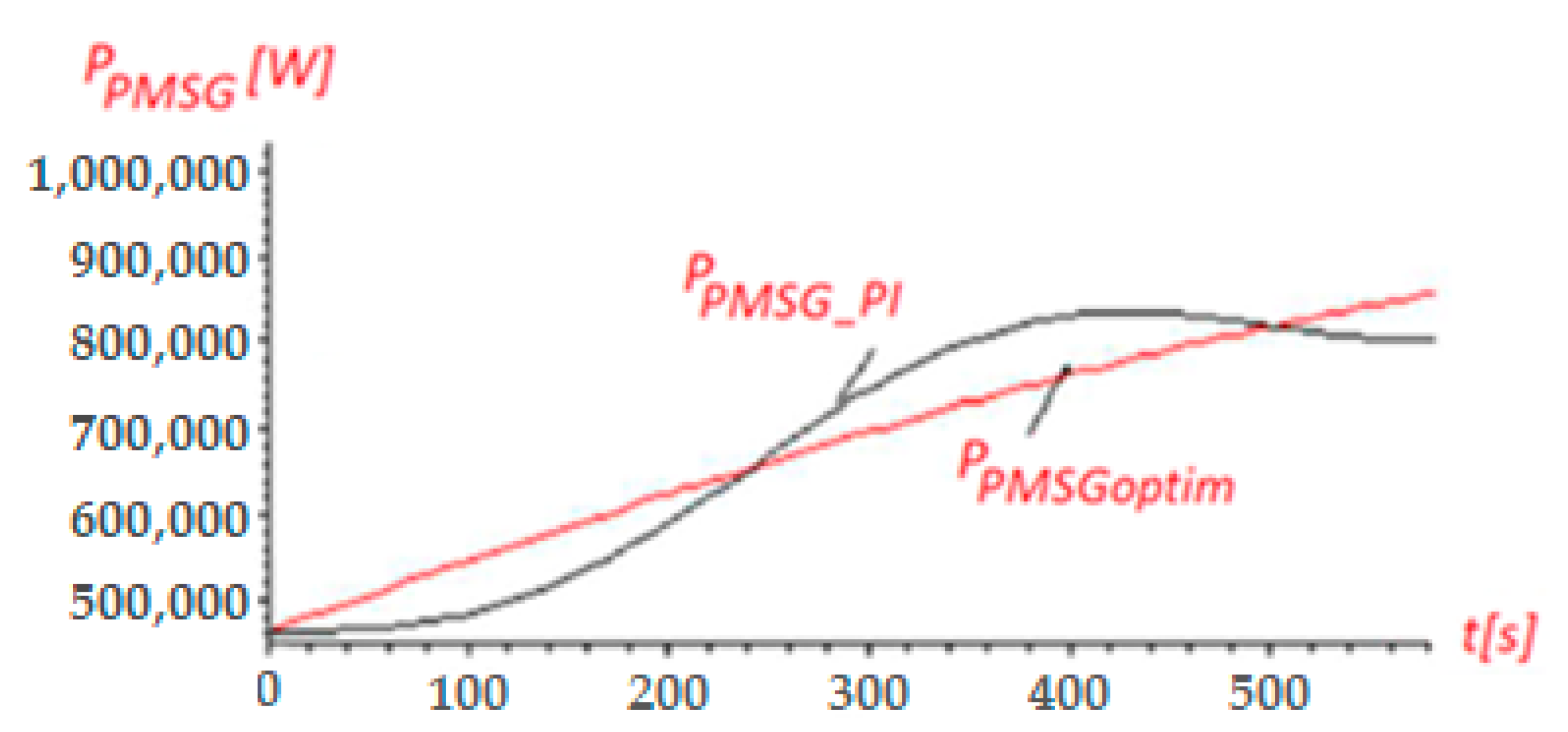
In conclusion, by using a PI-type regulator, the resulting PMSG optimal power, , oscillates around the optimal values of the , with amplitudes up to , as can be seen in Figure 3.
6.3. PID-Based Control of the PMSG’s Optimal Power
For the case study in this paragraph, the same experimental data are used as those used for the previous case studies. Therefore, the system of differential equations in Equation (33) becomes
The second order derivative of the wind speed time-varying curve, , is obtained by derivation of Equation (45):
Then, by replacing the wind speed time-varying curve, , its first order derivative, , and its second order derivative, , from Equations (44), (45) and (64), respectively, the below system of differential equations is obtained, as:
The initial conditions of the differential equations system in Equation (65) are calculated for the wind speed value from Table 1, corresponding to (s). Their expressions are the following ones:
The values of the proportional constant, , of the integral constant, , and of the derivative constant are also determined through the trial and error tuning method, so that the power oscillations are as small as possible, and the PMSG’s angular speed value, ω, is made to tend to the optimal value of the PMSG’s angular speed, . For example, at (s), the PMSG’s angular speed value is (rad/s) and (rad/s).
From the simulations, it results that the PMSG’s power oscillations are lowest for , as can also be seen in Figure 4, and using those from Equation (65) together with the initial conditions in Equation (66), the equations system in Equation (65) becomes
the solutions of which are the and curves.
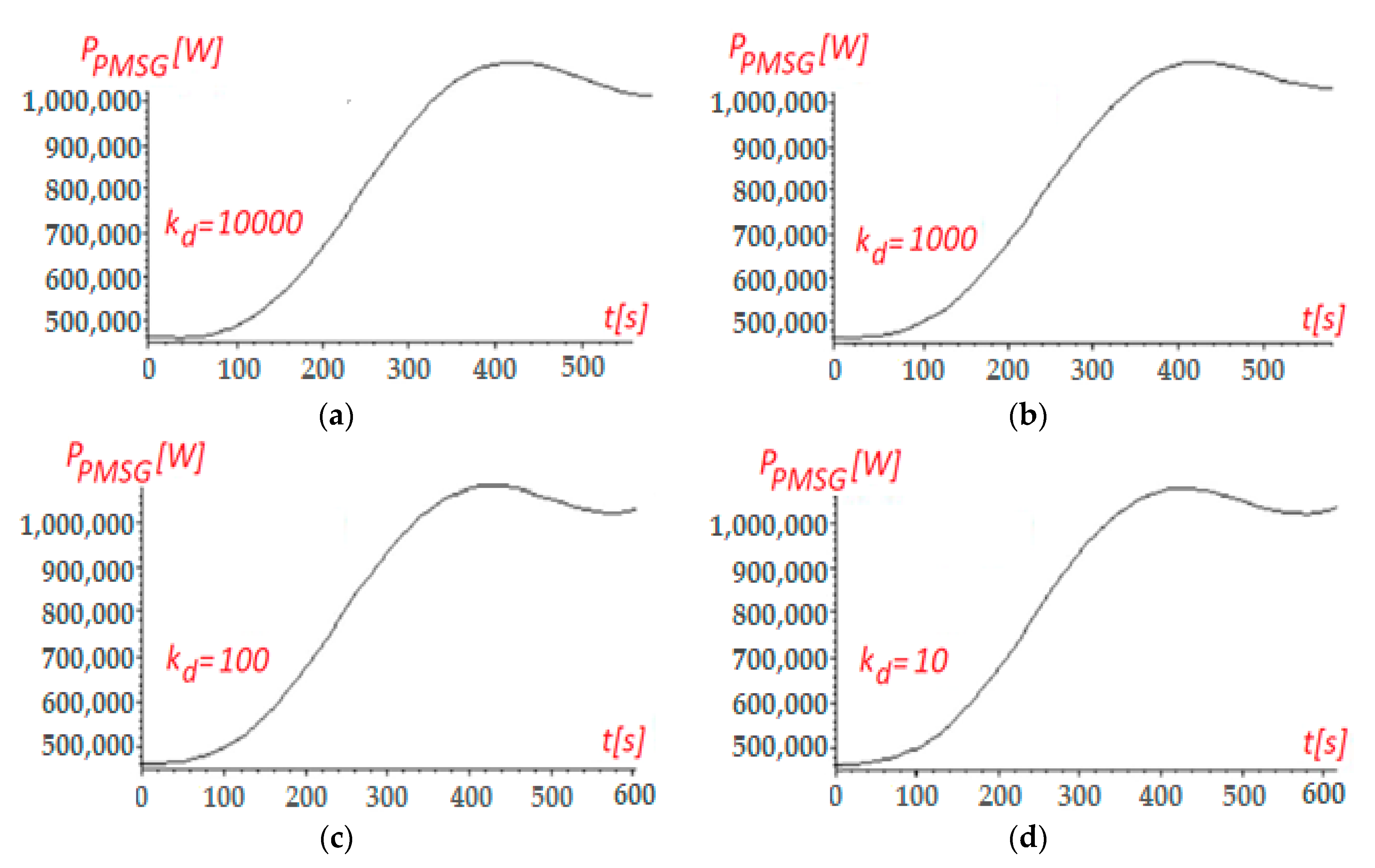
In order to highlight the influence of the derivative constant value, , on the time variation of the PMSG’s optimal power, when using a PID-type regulator, , several simulations, the results of which are given in Figure 4, were performed for different values of .
From the PMSG’s power time variation presented in Figure 4, it can be noticed that the power oscillations are not diminished when using a PID-type regulator instead of a PI-type regulator, regardless of the derivative constant value, . For , the PMSG’s optimal power curve, , obtained using a PID-based control, has the smallest oscillations around the PMSG’s optimal power curve , which result from the kinetic motion equation.
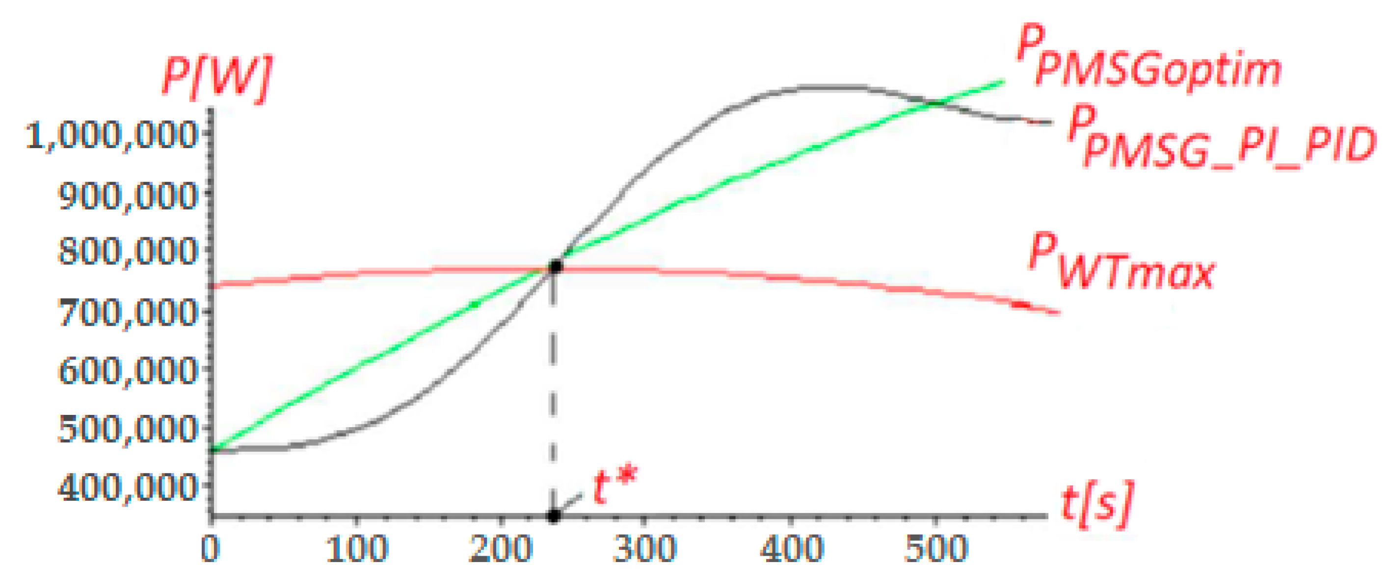
Figure 5 shows, by comparison, the time variations of the three powers described below:
- the maximum wind turbine’s power when operating at MPP, defined in Equation (47) ()
- the PMSG’s optimal power calculated from the kinetic motion equation, defined in Equation (49) ()
- the PMSG’s power obtained by using either the PI- or PID-type regulators, , resulting from either Equation (62) or Equation (67).
Remark 5: The derivative response is proportional to the rate of change of the process variable. Increasing the derivative component will cause the control system to react more rapidly to error. Thus, the derivative term allows one to have bigger P and I coefficients and still keep the loop stable, providing a faster response and a better loop performance. On the other hand, it can cause the output to decrease if the process variable is increasingly rapidly. Most practical control systems use very small derivative times, because the derivative response is very sensitive to noise, and it can make the control system unstable. So, the PI regulator is recommended, unless the process variable is really slow (as in this paper’s presented case, due to the large inertia).
Figure 6 shows the time variation of the PMSG’s angular speed, , and the derivative of the wind speed, .
Remark 6: At the moment, the derivative of the wind speed is canceled (see Figure 6), and the PMSG’s angular speed, , reaches its maximum, .
Thus, the wind speed and the PMSG’s angular speed reach their maximum values in the same time instant. Furthermore, the inertial power , yielding to the equality between the PMSG’s power and the wind turbine’s power, .
Therefore, by using the PI- or the PID-type regulators, the PMSG’s power oscillations increase, and they are dependent on the values of the constants.
For , the PMSG’s power oscillations have the smallest values, for wind speeds varying between 6.24 (m/s) and 6.32 (m/s).
As a general conclusion, it can be said that the two proposed controls bring the wind turbine within the MPP operation area, while is not identical to , but close to it.
7. Conclusions
In this paper, the operation of one wind turbine within a wind farm, the data for which is collected in [21], is analyzed for wind speed values measured with a sampling step of 30 s.
The operation of the wind turbine was analyzed at MPP, in which case the PMSG’s angular speed tends towards its optimal value. The PMSG’s optimal power values are determined by employing the values of the wind speed and its derivative in the mathematical model of the wind turbine. Since the wind turbine’s mathematical model is used to calculate the PMSG’s optimal angular speed’s dependence on the wind speed, its moment of total inertia should be considered.
For the actual PMSG’s angular speed, the wind turbine’s moment of total inertia behaves like a damper. Due to its high value, it is not possible for the PMSG to permanently operate at MPP, which, from the energy point of view, imposes the optimal value of the PMSG’s angular speed, because the PMSG’s angular speed is not capable of following the rapid variation of the wind speed in time.
Therefore, in order to capture the maximum wind energy, the wind turbine should be controlled to operate at the PMSG’s optimal angular speed, imposed by the wind speed value. This condition is checked periodically, and if there are large differences between the PMSG’s angular speed and its optimal value, the wind turbine is brought into the MPP operation by inserting the necessary amount of electric energy, provided by the national power system. If the value of the wind speed is decreasing, its derivate becomes negative, and the PMSG’s power becomes greater than the wind turbine’s power, while in the case of the wind speed increasing, its derivative becomes positive, and the PMSG’s power becomes lower than that of the wind turbine’s power value.
Thus, two methods to direct the PMSG’s power towards its optimal value were proposed herein, both of them based on the same principle, using either a PI-type regulator or a PID-type regulator.
The values of the regulator coefficients are determined by successive simulations, so that the oscillations of the power are reduced. The simulations are actually the numerical solutions obtained by using the MAPLE core of the Scientific Workplace simulation environment, and they are based on the wind speed measurements.
In conclusion, it can be said that the proposed controls can bring the wind turbine within the MPP operation area. However, the PMSG’s power, based on either the PI- or PID-type control, is not identical to the theoretical PMSG’s optimal power based on the kinetic motion equation, but close to it, depending on the applied control method.
For the presented case study, where the moment of total wind turbine inertia is large and leads to reduced dynamics in the wind turbine’s operation, the PID regulator is recommended.
For practical application, the obtained PMSG’s optimal power curve is useful for monitoring and increasing the performance of the wind turbines. As was shown in this paper, the PMSG’s optimal power curve can be extracted from the wind speed measurements data. This curve can be used as a reference curve. The actual PMSG’s power curve to be monitored can be compared with the reference one, and the wind turbine can then be controlled, so that the deviation of the actual values from the expected ones will be as small as possible, which increases the wind turbine’s efficiency.
Author Contributions
Writing—original draft preparation, M.-C.A.; Conceptualization, S.M.; Methodology, S.M.; Software, C.S.; Validation, M.-C.A., M.D. and C.S.; Formal analysis, G.M.E.; Investigation, M.D.; Resources, G.M.E.; Data curation, C.S.; Writing—review and editing, M.-C.A.; Visualization, M.D.; Supervision, M.-C.A.; Project administration, S.M. All authors have read and agreed to the published version of the manuscript.
Funding
This research was funded by University POLITEHNICA Timisoara, GNaC2018 ARUT, no.1357/01.02.2019.
Conflicts of Interest
The authors declare no conflict of interest.
Nomenclature
PI—proportional integrator; PID—proportional integrator derivative; MPP—maximum power point; PMSG—permanent magnet synchronous generator; WT—wind turbine; WTPC—the wind turbine power curves.
Appendix A

Table A1.
Technical specifications of the GE 2.5 (MW) wind turbine.
| Type | Horizontal Axis Wind Turbine with Variable Rotor Speed |
|---|---|
| Rotor diameter | 100 m |
| Power regulation | Independent electromechanical pitch system for each blade |
| Rated power | 2500 kW |
| Hub height | 100 m |
| Rated rotational speed | 14.05 rpm |
| Operating range rotational speed | 3.83–15.61 rpm |
| Cut-in wind speed | 3 m/s |
| Rated wind speed | 12 m/s |
| Cut-out wind speed (10-min mean) | 25 m/s |
| Extreme wind speed (50-year mean) | 37.5 m/s |
| Annual average wind speed | 7.5 m/s |
| Design life time | 20 years |
| IEC 61400-1, class | IIIA |
Table A2.
List of the variables used in the paper.
| Variable | Description | Units |
|---|---|---|
| delivered energy | (J) | |
| captured wind energy | (J) | |
| kinetic energy | (J) | |
| total moment of inertia | () | |
| inertial power | (W) | |
| PMSG’s power | (W) | |
| PMSG’s average power | (W) | |
| PMSG’s optimal power | (W) | |
| PMSG’s power obtained by using either the PI- or PID-type regulators | (W) | |
| PMSG’s power in the case of PI control | (W) | |
| PMSG’s power in the case of PID control | (W) | |
| wind turbine’s power | (W) | |
| wind turbine’s average power | (W) | |
| wind turbine’s maximum power | (W) | |
| PMSG’s torque | (Nm) | |
| wind turbine’s torque | (Nm) | |
| wind speed | (m/s) | |
| measured wind speed | (m/s) | |
| PMSG’s angular speed | (rad/s) | |
| PMSG’s maximum angular speed | (rad/s) | |
| PMSG’s optimal angular speed | (rad/s) | |
| the PMSG’s angular speed at time instant | (rad/s) | |
| the PMSG’s angular speed at time instant | (rad/s) |
References
- Qi, L.; Zheng, L.; Bai, X.; Chen, Q.; Chen, J.; Chen, Y. Chen Nonlinear Maximum Power Point Tracking Control Method for Wind Turbines Considering Dynamics. Appl. Sci. 2020, 10, 811. [Google Scholar] [CrossRef] [Green Version]
- Sorandaru, C.; Musuroi, S.; Ancuti, M.-C.; Erdodi, G.-M.; Petrescu, D.-I. Equivalent power for a wind power system. In Proceedings of the 2016 IEEE 11th International Symposium on Applied Computational Intelligence and Informatics (SACI), Timisoara, Romania, 12–14 May 2016; pp. 225–228. [Google Scholar] [CrossRef]
- Sorandaru, C.; Musuroi, S.; Frigura-Iliasa, F.M.; Vatau, D.; Dordescu, M. Analysis of the Wind System Operation in the Optimal Energetic Area at Variable Wind Speed over Time. Sustainability 2019, 11, 1249. [Google Scholar] [CrossRef] [Green Version]
- Abdullah, M.; Yatim, A.H.; Tan, C.; Saidur, R. A review of maximum power point tracking algorithms for wind energy systems. Renew. Sustain. Energy Rev. 2012, 16, 3220–3227. [Google Scholar] [CrossRef]
- Hussein, M.M.; Senjyu, T.; Orabi, M.; Wahab, M.A.A.; Hamada, M.M. Control of a Stand-Alone Variable Speed Wind Energy Supply System. Appl. Sci. 2013, 3, 437–456. [Google Scholar] [CrossRef] [Green Version]
- Yin, M.; Li, W.; Chung, C.Y.; Zhou, L.; Chen, Z.; Zou, Y. Optimal torque control based on effective tracking range for maximum power point tracking of wind turbines under varying wind conditions. IET Renew. Power Gener. 2017, 11, 501–510. [Google Scholar] [CrossRef]
- Yang, Z.; Yin, M.; Xu, Y.; Zou, Y.; Dong, Z.Y.; Zhou, Q. Inverse Aerodynamic Optimization Considering Impacts of Design Tip Speed Ratio for Variable-Speed Wind Turbines. Energies 2016, 9, 1023. [Google Scholar] [CrossRef] [Green Version]
- Seo, S.; Oh, S.-D.; Kwak, H.-Y. Wind turbine power curve modeling using maximum likelihood estimation method. Renew. Energy 2019, 136, 1164–1169. [Google Scholar] [CrossRef]
- Marčiukaitis, M.; Žutautaitė, I.; Martišauskas, L.; Jokšas, B.; Gecevičius, G.; Sfetsos, A. Non-linear regression model for wind turbine power curve. Renew. Energy 2017, 113, 732–741. [Google Scholar] [CrossRef]
- Taslimi-Renani, E.; Delshad, M.M.; Elias, M.F.M.; Rahim, N.A. Development of an enhanced parametric model for wind turbine power curve. Appl. Energy 2016, 177, 544–552. [Google Scholar] [CrossRef]
- Linus, R.M.; Damodharan, P. Maximum power point tracking method using a modified perturb and observe algorithm for grid connected wind energy conversion systems. IET Renew. Power Gener. 2015, 9, 682–689. [Google Scholar] [CrossRef]
- Karabacak, M.; Fernández-Ramírez, L.M.; Kamal, T.; Kamal, S. A New Hill Climbing Maximum Power Tracking Control for Wind Turbines With Inertial Effect Compensation. IEEE Trans. Ind. Electron. 2019, 66, 8545–8556. [Google Scholar] [CrossRef]
- Noorollahi, Y.; Jokar, M.A.; Kalhor, A. Using artificial neural networks for temporal and spatial wind speed forecasting in Iran. Energy Convers. Manag. 2016, 115, 17–25. [Google Scholar] [CrossRef]
- Wei, C.; Zhang, Z.; Qiao, W.; Qu, L. An Adaptive Network-Based Reinforcement Learning Method for MPPT Control of PMSG Wind Energy Conversion Systems. IEEE Trans. Power Electron. 2016, 31, 7837–7848. [Google Scholar] [CrossRef]
- Navarrete, E.C.; Trejo-Perea, M.; Correa, J.C.J.; Carrillo-Serrano, R.V.; Ríos-Moreno, J.G. Expert Control Systems for Maximum Power Point Tracking in a Wind Turbine with PMSG: State of the Art. Appl. Sci. 2019, 9, 2469. [Google Scholar] [CrossRef] [Green Version]
- Zuluaga, C.; Álvarez, M.A.; Giraldo, E. Short-term wind speed prediction based on robust Kalman filtering: An experimental comparison. Appl. Energy 2015, 156, 321–330. [Google Scholar] [CrossRef]
- Beltran, O.; Peña, R.; Ramírez, J.S.; Esparza, A.; Muljadi, E.; Gao, W. Inertia Estimation of Wind Power Plants Based on the Swing Equation and Phasor Measurement Units. Appl. Sci. 2018, 8, 2413. [Google Scholar] [CrossRef] [Green Version]
- Shang, L.; Hu, J.; Yuan, X.; Chi, Y. Understanding Inertial Response of Variable-Speed Wind Turbines by Defined Internal Potential Vector. Energies 2016, 10, 22. [Google Scholar] [CrossRef]
- Yang, B.; Yu, T.; Shu, H.; Dong, J.; Jiang, L. Robust sliding-mode control of wind energy conversion systems for optimal power extraction via nonlinear perturbation observers. Appl. Energy 2018, 210, 711–723. [Google Scholar] [CrossRef]
- Liu, X.; Han, Y.; Wang, C. Second-order sliding mode control for power optimisation of DFIG-based variable speed wind turbine. IET Renew. Power Gener. 2017, 11, 408–418. [Google Scholar] [CrossRef]
- Available online: http://www.monsson.eu (accessed on 10 December 2019).
Figure 1.
Time variations of the approximated wind speed, , of its derivative, , and of the measured the wind speed, .
Figure 1.
Time variations of the approximated wind speed, , of its derivative, , and of the measured the wind speed, .
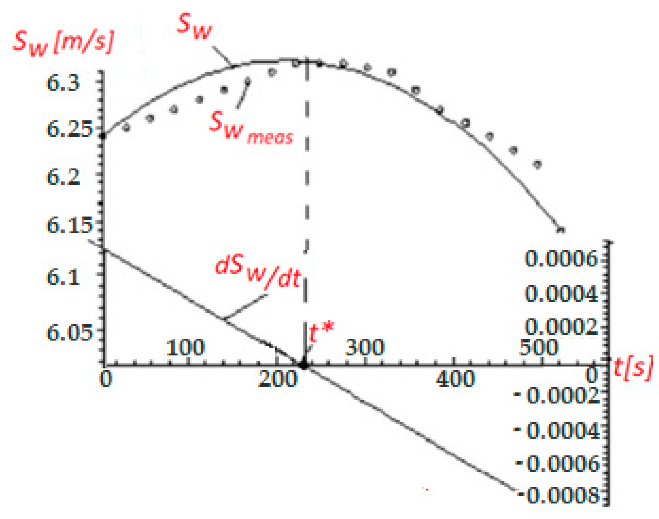
Figure 2.
Powers variations in time: and .

Figure 3.
Powers variations in time: and .

Figure 4.
Time variation of the optimal PMSG‘s power curve, for: (a). , (b). , (c). , (d). , (e). , (f). , (g). , (h). .
Figure 4.
Time variation of the optimal PMSG‘s power curve, for: (a). , (b). , (c). , (d). , (e). , (f). , (g). , (h). .

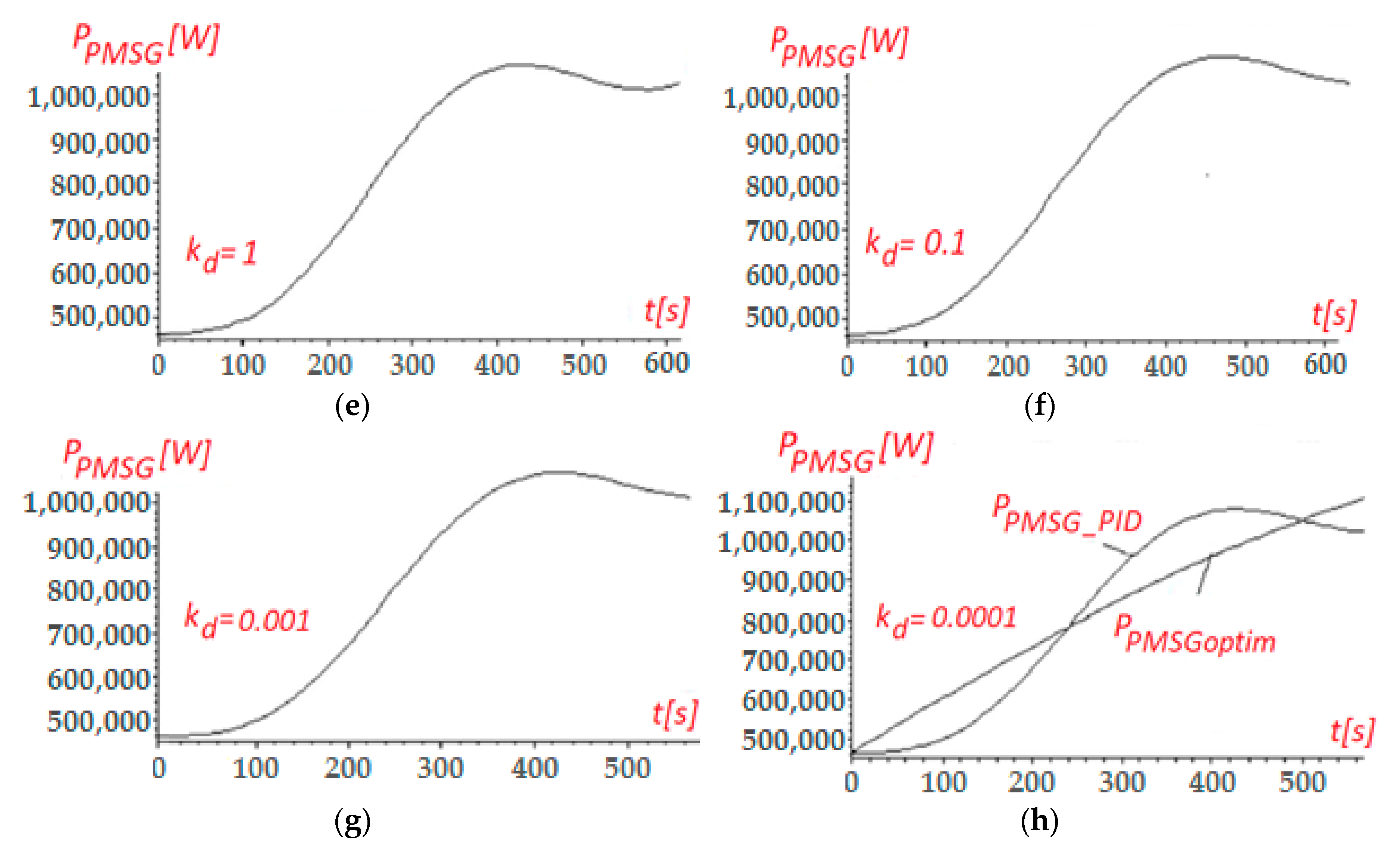
Figure 5.
Time variation of the three power curves: , and .

Figure 6.
Time variation of the PMSG’s angular speed and of the wind speed derivative .
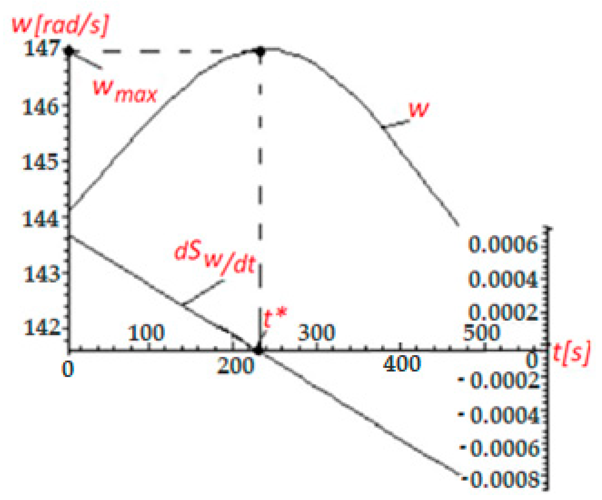
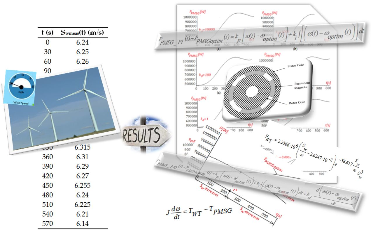
Table 1.
Measured wind speed values over time.
| t (s) | Swmeas(t) (m/s) |
|---|---|
| 0 | 6.24 |
| 30 | 6.25 |
| 60 | 6.26 |
| 90 | 6.27 |
| 120 | 6.28 |
| 150 | 6.29 |
| 180 | 6.3 |
| 210 | 6.31 |
| 240 | 6.32 |
| 270 | 6.32 |
| 300 | 6.32 |
| 330 | 6.315 |
| 360 | 6.31 |
| 390 | 6.29 |
| 420 | 6.27 |
| 450 | 6.255 |
| 480 | 6.24 |
| 510 | 6.225 |
| 540 | 6.21 |
| 570 | 6.14 |
© 2020 by the authors. Licensee MDPI, Basel, Switzerland. This article is an open access article distributed under the terms and conditions of the Creative Commons Attribution (CC BY) license (http://creativecommons.org/licenses/by/4.0/).
Share and Cite
MDPI and ACS Style
Ancuti, M.-C.; Musuroi, S.; Sorandaru, C.; Dordescu, M.; Erdodi, G.M. Wind Turbines Optimal Operation at Time Variable Wind Speeds. Appl. Sci. 2020, 10, 4232. https://doi.org/10.3390/app10124232
AMA Style
Ancuti M-C, Musuroi S, Sorandaru C, Dordescu M, Erdodi GM. Wind Turbines Optimal Operation at Time Variable Wind Speeds. Applied Sciences. 2020; 10(12):4232. https://doi.org/10.3390/app10124232
Chicago/Turabian StyleAncuti, Mihaela-Codruta, Sorin Musuroi, Ciprian Sorandaru, Marian Dordescu, and Geza Mihai Erdodi. 2020. "Wind Turbines Optimal Operation at Time Variable Wind Speeds" Applied Sciences 10, no. 12: 4232. https://doi.org/10.3390/app10124232
Note that from the first issue of 2016, this journal uses article numbers instead of page numbers. See further details here.