Optimal Design of Adaptive Robust Control for the Delta Robot with Uncertainty: Fuzzy Set-Based Approach

Abstract

An optimal control design for the uncertain Delta robot is proposed in the paper. The uncertain factors of the Delta robot include the unknown dynamic parameters, the residual vibration disturbances and the nonlinear joints friction, which are (possibly fast) time-varying and bounded. A fuzzy set theoretic approach is creatively used to describe the system uncertainty. With the fuzzily depicted uncertainty, an adaptive robust control, based on the fuzzy dynamic model, is established. It designs an adaptation mechanism, consisting of the leakage term and the dead-zone, to estimate the uncertainty information. An optimal design is constructed for the Delta robot and solved by minimizing a fuzzy set-based performance index. Unlike the traditional fuzzy control methods (if-then rules-based), the proposed control scheme is deterministic and fuzzily optimized. It is proven that the global solution in the closed form for this optimal design always exists and is unique. This research provides the Delta parallel robot a novel optimal control to guarantee the system performance regardless of the uncertainty. The effectiveness of the proposed control is illustrated by a series of simulation experiments. The results reveal that the further applications in other robots are feasible.

1. Introduction

Delta robot, one of the most successful parallel mechanisms, has been widely applied in many sophisticated fields, such as microelectronics [1,2,3], medicine [4,5], intelligent logistics [6,7] and 3D printing [8,9]. It inherits not only all the virtues of the traditional parallel robot, but also possesses some unique features such as lighter weight, faster motion, higher efficiency and larger payload capacity, which are elaborated in [10,11]. Due to those additional merits, certain nonlinear and uncertain factors in Delta robot could affect the system performance (e.g., accuracy and speed) and can not be ignored, such as the nonlinear joints friction, the random external loads, the residual vibration caused by the effect of the lightweight material and so on, which significantly enhance the difficulty of the control design. Hence, the control of Delta robot with high nonlinearities and uncertainty seems attractive and appealing for researchers [12,13].

In recent years, many control designs are proposed for Delta robot with uncertainty, such as [14] designed a $H_{\infty }$ feedback controller to ensure the trajectory accuracy of a 3-DOF Delta robot with random work loads in pick and place operation; Ref. [15] presented a tracking control for the Delta robot manipulator with external disturbances by employing the fractional order PID controllers; Based on a linear disturbance observation, an active disturbance rejection controller was constructed to ease the presence of the possible noise effects in Delta robot [16]; Ref. [17] discussed the tracking problem for Delta robot with uncertain parameters by using an adaptive control algorithm; Ref. [18] analyzed the mechanical vibrations issue in the Par2-Delta parallel robot and proposed an adaptive dual mode controller to solve it. Furthermore, some intelligent control methods have also been adopted for controlling the Delta robot by function approximation or fitness selection, for example the neural network control in [19] and the fuzzy control method in [20,21].

Most of the present control approaches devote to tackle the uncertainty of Delta robot from the perspectives of investigating the stochastic properties of the uncertain terms (such as, [14,15]) or on-line estimating the uncertain parameters (see, i.e., [16,17,18]). However, in this paper, a fuzzy set theoretic approach is proposed to explore the uncertainty in Delta robot, and can be considered as the third perspective. The uncertainty information of Delta robot is depicted by the fuzzy sets theory, which is unknown but is within a fuzzy threshold. Based on the fuzzy description of uncertainty, a deterministic control design is constructed. It is a new way to combine the fuzzy set theory and control theory of Delta robot, and does not belong to the traditionally if-then rules-based fuzzy control design framework in [22,23,24,25,26,27,28].

The main contributions of this work are threefold. First, the uncertain factors of Delta robot are novelly described by a fuzzy set theoretic approach. Based on the fuzzy uncertainty, we reformulate the dynamic modeling of Delta robot, which is nonlinear and not Takagi-Sugeno type modeling (using fractional linearization). Second, we propose a fuzzy performance index for Delta robot to optimize the adaptive robust control gain. The performance index considers the impacts of the transient performance, the steady state performance and the control cost. The Delta robot controller with optimized gain is deterministic and is not the if-then rules-based or Mamdani-type fuzzy control. Third, through the defuzzification of the performance index, the solution of the optimal control design is proven to exist and be unique, which is resolved in the closed form. Under the optimal control design, both deterministic (uniform boundedness and uniform ultimate boundedness) and fuzzy (minimizing the fuzzy performance index) performance of Delta robot could be guaranteed.

2. Fuzzy Preliminaries

The following mathematical preliminaries are needed for the follow-up control work and optimization design.

Decomposition theorem: ${\tilde{D}}_o$ is considered to be a fuzzy set in H. ${\mu }_{{\tilde{D}}_o}=o{I}_{{\tilde{D}}_o}\left(h\right)$ is the membership function where $I_{{\tilde{D}}_o}\left(h\right)=1$ if $h\in \widetilde{D_o}$ and $I_{{\tilde{D}}_o}\left(h\right)=0$ if $h\in H-{\tilde{D}}_o$. Then the fuzzy set D is given by

$$\begin{array}{c}\hfill D=\bigcup _{o\in [0,1]}{\tilde{D}}_o,\end{array}$$

(1)

where ⋃ is the union operation of the fuzzy sets. With these, the membership function can be constructed by using the decomposition theorem after the algebraic operation of fuzzy numbers [29].

D-operation: $\mathcal{X}=\left\{(s,{\mu }_X)\right|s\in X\}$ is considered to be a fuzzy set. For each function $f:X\to \mathbf{R}$, the D-operation is given by

$$\begin{array}{c}\hfill D\left[f\left(s\right)\right]=\frac{{\int }_{X}f\left(s\right){\mu }_X\left(s\right)ds}{{\int }_X{\mu }_X\left(s\right)ds}.\end{array}$$

(2)

Remark 1.

The D-operation is essentially a procedure to find the average value of $f\left(s\right)$ over ${\mu }_X\left(s\right)$. Note that if $f\left(s\right)=s$, the operation can be simplified to the center-of-gravity defuzzification method [30]. Additionally, if $\mathcal{X}$ is crisp (i.e., ${\mu }_X\left(s\right)=1$), then $D\left[f\left(s\right)\right]=f\left(s\right)$.

3. Adaptive Robust Control Design

The problem in this research is formulated as twofold: in virtue of fuzzy dynamic systems, exploring a novel robust control to regulate the Delta robot with the highly nonlinear dynamics and the uncertain factors; based on the fuzzy information of the uncertainty, optimizing the proposed robust control by considering the control cost and system performance. In this section, a robust control with adaptive mechanism is proposed. First, the fuzzy dynamic model of Delta robot is introduced. Then, the effectiveness of the adaptive robust control scheme is verified by a theorem.

3.1. Fuzzy Dynamic Modeling of Delta Robot

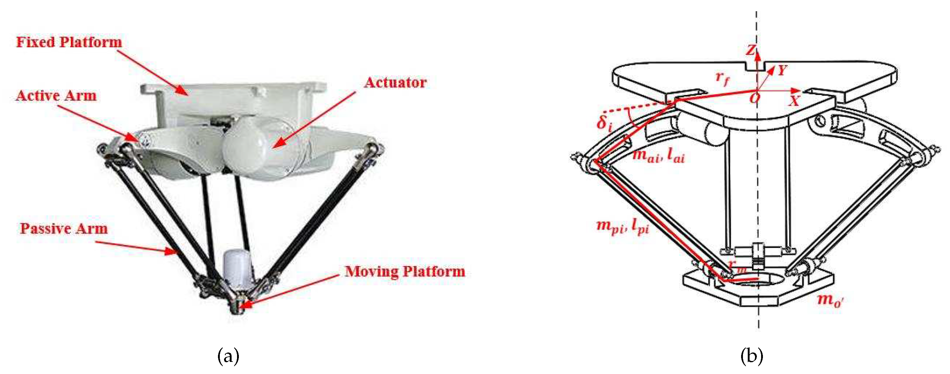
A 3-DOF Delta robot, with three common RRPaR (R denotes the rotation pair, Pa is the parallelogram configuration) topology mechanisms connecting the fixed platform and the moving platform, is taken into consideration. The sub-chains with active arms and passive arms are located on the three sides of an equilateral triangle, which are presented in Figure 1a.

Assign a base frame $O\{X,Y,Z\}$ at the geometric center of the fixed platform in Figure 1b, and denote the parameters in the

Table 1. Parameters of Delta robot.

Description	Notation	Units
Angle of the i-th active joint	${\delta }_i$	rad
Length of the i-th active arm	$l_{ai}$	m
Length of the i-th passive arm	$l_{pi}$	m
Radius of the fixed platform	$r_f$	m
Radius of the moving platform	$r_m$	m
Mass of the i-th active arm	$m_{ai}$	kg
Mass of the i-th passive arm	$m_{pi}$	kg
Mass of the moving platform	$m_{o^{{}^{\prime }}}$	kg

$(i=1,2,3)$:

Select $\delta ={[{\delta }_1,{\delta }_2,{\delta }_3]}^T$ as the generalized coordinate vector. Based on the dynamics constructed in [31], the motion equation of Delta robot with uncertainty can be formulated as

$$\begin{array}{cc}\hfill M(\delta \left(t\right),\varsigma \left(t\right),t)\ddot{\delta }\left(t\right)& +C(\delta \left(t\right),\dot{\delta }\left(t\right),\varsigma \left(t\right),t)\dot{\delta }\left(t\right)+G(\delta \left(t\right),\varsigma \left(t\right),t)\hfill \\ \hfill & +F_e(\delta \left(t\right),\dot{\delta }\left(t\right),\varsigma \left(t\right),t)+M_f(\delta \left(t\right),\dot{\delta }\left(t\right),\varsigma \left(t\right),t)=\tau \left(t\right),\hfill \end{array}$$

(3)

where $t\in \mathbf{R}$ is time, $\dot{\delta }\left(t\right)\in {\mathbf{R}}^n$ is the velocity, $\ddot{\delta }\left(t\right)\in {\mathbf{R}}^n$ is the acceleration. $\varsigma \left(t\right)\in \mathsf{\Sigma }\subset {\mathbf{R}}^p$ is the bounded uncertain parameters, $\mathsf{\Sigma }$ represents the possible bound of $\varsigma$, which is compact but unknown. $M\left(\delta \right(t),\varsigma (t),t)$ is the inertial matrix, $C(\delta \left(t\right),\dot{\delta }\left(t\right),\varsigma \left(t\right),t)$ is the Coriolis/centrifugal force, $G\left(\delta \right(t),\varsigma (t),t)$ is the gravitation force, $F_e(\delta \left(t\right),\dot{\delta }\left(t\right),\varsigma \left(t\right),t)$ stands for the external disturbances, $M_f(\delta \left(t\right),\dot{\delta }\left(t\right),\varsigma \left(t\right),t)$ represents the joint frictional moment, and $\tau \left(t\right)\in {\mathbf{R}}^n$ is the control torques. For simplicity, the argument will be omitted without ambiguity. The detail expressions of $M(·)$, $C(·)$ and $G(·)$ are shown in Appendix A.

For a Delta robot, the actuators are installed in the active joints, which are generally composed of drive motors and harmonic reducers. The addition of the harmonic reducers not only leads to the flexibility of the joints, but also increases the complexity of internal joints friction. Therefore, in this paper, the friction of the active joints is considered.

The frictional moment during the transmission process of the harmonic reducer is mainly related to the joint speed and direction. A Stribeck friction model, which conforms to the friction characteristics in the transmission process, is used to model the joints friction of Delta robot, and the model is given by [32]

$$\begin{array}{cc}\hfill M_f& =\left[F_c+(F_s-F_c)e^{-{(\dot{\delta }/{\dot{\delta }}_s)}^2}\right]\mathrm{sgn}\left(\dot{\delta }\right)r_a+{\mu }_v\dot{\delta }{r}_a,\hfill \\ \hfill F_c& ={\mu }_d{F}_n,F_s={\mu }_s{F}_n,\hfill \end{array}$$

(4)

where $F_c$ is Coulomb friction, $F_s$ is the stiction friction, ${\delta }_s$ is Stribeck velocity, ${\mu }_v$ is the coefficient of the viscous friction, ${\mu }_d$ is the coefficient of Coulomb friction, ${\mu }_s$ is the coefficient of static friction, $F_n$ is the normal force, $r_a$ is the friction arm of the active joints.

Remark 2.

The dimension of the uncertain factors $\varsigma \in \mathsf{\Sigma }\subset {\mathbf{R}}^p$ is determined by the number of the uncertain terms in Delta robot. Each of them is compact and bounded. Due to the uncertainty, the determination of the matrix $M(·)$, $C(·)$, $G(·)$, $F_e(·)$ and $M_f(·)$ are associated with not only the generalized coordinate δ and the generalized velocity $\dot{\delta }$ but also the uncertainty parameter ς.

Assumption 1.

The matrix $M(\delta ,\varsigma ,t)$ is uniformly positive definite, which leads to

$$M(\delta ,\varsigma ,t)>\sigma I$$

(5)

for all $\delta \in {\mathbf{R}}^n$. Here, $\sigma >0$ is a scalar constant.

Remark 3.

In the past, Assumption 1 was generally considered to be a fact rather than an assumption [33]. However, in some mechanical systems, the matrix $M(\delta ,\varsigma ,t)$ is proved to be a semi-positive definite matrix under some circumstances. Some examples are listed in [34].

Assumption 2.

For all $\delta \in {\mathbf{R}}^n$, $\varsigma \in \mathsf{\Sigma }$, the matrix $M(\delta ,\varsigma ,t)$ is bounded as

$$\parallel M(\delta ,\varsigma ,t)\parallel \le {\kappa }_0+{\kappa }_1\parallel \delta \parallel +{\kappa }_2{\parallel \delta \parallel }^2.$$

(6)

Here, ${\kappa }_x$ are scalar constants, $x=0,1,2$, ${\kappa }_0>0$, ${\kappa }_{1,2}\ge 0$.

Remark 4.

For any rigid type robots with revolute and slide joints, $M(\delta ,\varsigma ,t)$ is related to the parameters of the inertia matrix and the positions of the joints, that is, there exists a set of constants ${\kappa }_x$, the euclidean norm of the inertia matrix satisfies (6).

There exist no slide joints but only revolute joints in Delta robot, which leads to ${\kappa }_1={\kappa }_2=0$ such that

$$\begin{array}{c}\hfill \parallel M(\delta ,\varsigma ,t)\parallel \le {\kappa }_0.\end{array}$$

(7)

Assumption 3.

(1) Suppose the initial state of Delta robot, which is uncertain, be expressed as ${\delta }_0={[\delta {\left(t_0\right)}^T,\dot{\delta }{\left(t_0\right)}^T]}^T$, where $t_0$ is the initial time. For any element in ${\delta }_0$, namely ${\delta }_{0i}$, $i=1,2,\cdots ,2n$, there exists a fuzzy set $U_{0i}$ in a universe of discourse ${\mathsf{\Lambda }}_i\in \mathbf{R}$ represented as

$$\begin{array}{c}\hfill U_{0i}=\left\{({\delta }_{0i},{\mu }_{{\mathsf{\Lambda }}_i}\left({\delta }_{0i}\right))|{\delta }_{0i}\in {\mathsf{\Lambda }}_i\right\}.\end{array}$$

(8)

Here, ${\mu }_{{\mathsf{\Lambda }}_i}:{\mathsf{\Lambda }}_i\to [0,1]$ is the membership function, ${\mathsf{\Lambda }}_i$ is known and compact.

(2) For any element in ς, namely ${\varsigma }_i,i=1,2,\cdots ,m$, the element ${\varsigma }_i(·)$ is Lebesgue measurable.

(3) For each ${\varsigma }_i$, there exists a fuzzy set $U_{1i}$ in the universe of discourse ${\mathsf{\Sigma }}_i\in \mathbf{R}$ represented as

$$\begin{array}{c}\hfill U_{1i}=\left\{({\varsigma }_i,{\mu }_{{\mathsf{\Sigma }}_i}\left({\varsigma }_i\right))\right|{\varsigma }_i\in {\mathsf{\Sigma }}_i\}.\end{array}$$

(9)

Here, ${\mu }_{{\mathsf{\Sigma }}_i}:{\mathsf{\Sigma }}_i\to [0,1]$ is the membership function, ${\mathsf{\Sigma }}_i$ is known and compact, $\mathsf{\Sigma }={\mathsf{\Sigma }}_1\times {\mathsf{\Sigma }}_2\times \cdots \times {\mathsf{\Sigma }}_m$.

3.2. Deign of Adaptive Robust Control for Delta Robot

Consider the trajectory tracking error of Delta robot described by

$$\begin{array}{c}\hfill r\left(t\right)=\delta \left(t\right)-{\delta }^d\left(t\right),\end{array}$$

(10)

where ${\delta }^d\left(t\right)$ is the desired trajectory, $t\in [t_0,t_1]$. Note that ${\delta }^d(·):[t_0,\infty ]\to {\mathbf{R}}^n$ is considered to be ${\mathbf{C}}^2$. Then $\dot{r}\left(t\right)=\dot{\delta }\left(t\right)-{\dot{\delta }}^d\left(t\right)$, $\ddot{r}\left(t\right)=\ddot{\delta }\left(t\right)-{\ddot{\delta }}^d\left(t\right)$. we assume that ${\delta }^d\left(t\right)$, ${\dot{\delta }}^d\left(t\right)$ and ${\ddot{\delta }}^d\left(t\right)$ are uniformly bounded.

Decompose the matrices $M(·)$, $C(·)$, $G(·)$, $F_e(·)$ and $M_f(·)$ in (3) as :

$$\begin{array}{cc}\hfill M(\delta ,\varsigma ,t)& =\overline{M}(\delta ,t)+\Delta M(\delta ,\varsigma ,t),\hfill \end{array}$$

(11)

$$\begin{array}{cc}\hfill C(\delta ,\dot{\delta },\varsigma ,t)& =\overline{C}(\delta ,\dot{\delta },t)+\Delta C(\delta ,\dot{\delta },\varsigma ,t),\hfill \end{array}$$

(12)

$$\begin{array}{cc}\hfill G(\delta ,\varsigma ,t)& =\overline{G}(\delta ,t)+\Delta G(\delta ,\varsigma ,t),\hfill \end{array}$$

(13)

$$\begin{array}{cc}\hfill F_e(\delta ,\dot{\delta },\varsigma ,t)& ={\overline{F}}_e(\delta ,\dot{\delta },t)+\Delta F_e(\delta ,\dot{\delta },\varsigma ,t),\hfill \end{array}$$

(14)

$$\begin{array}{cc}\hfill M_f(\delta ,\dot{\delta },\varsigma ,t)& ={\overline{M}}_f(\delta ,\dot{\delta },t)+\Delta M_f(\delta ,\dot{\delta },\varsigma ,t).\hfill \end{array}$$

(15)

Here, the matrices $\overline{M}$, $\overline{C}$, $\overline{G}$, ${\overline{F}}_e$ and ${\overline{M}}_f$ are referred to as the “norm” portions, the matrices $\Delta M$, $\Delta C$, $\Delta G$, $\Delta F_e$ and $\Delta M_f$ are referred to as the uncertain portions which are associated with $\varsigma$.

Assumption 4.

(1) For all $(\delta ,\dot{\delta },t),\varsigma \in \mathsf{\Sigma }$, there exists a given function $\mathsf{\Gamma }(·):{(0,\infty )}^k\times {\mathbf{R}}^n\times {\mathbf{R}}^n\times \mathbf{R}\to {\mathbf{R}}_{+}$ such that

$$\parallel \omega (r,\dot{r},\varsigma ,t)\parallel \le \mathsf{\Gamma }(\rho ,\delta ,\dot{\delta },t),$$

(16)

where

$$\begin{array}{cc}\hfill \omega (r,\dot{r},\varsigma ,t)=& -\Delta M(\delta ,\varsigma ,t)\left({\ddot{\delta }}^d-A\dot{r}\right)-\Delta C(\delta ,\dot{\delta },\varsigma ,t)\left({\dot{\delta }}^d-Ar\right)-\Delta G(\delta ,\varsigma ,t)\hfill \\ \hfill & -\Delta F_e(\delta ,\dot{\delta },\varsigma ,t)-\Delta M_f(\delta ,\dot{\delta },\varsigma ,t).\hfill \end{array}$$

(A1)

Here, A = $\mathrm{diag}$${\left[a_i\right]}_{\mathrm{n}\times \mathrm{n}}$, $a_i>0$, $i=1,2,\cdots ,n$, $\rho \in {(0,\infty )}^k$ is a constant vector.

(2) For any element in ρ, namely ${\rho }_i,i=1,2,\cdots ,k$, there exists a fuzzy set $U_{2i}$ in a universe of discourse ${\mathsf{\Omega }}_i\in \mathbf{R}$ represented as

$$\begin{array}{c}\hfill U_{2i}=\left\{({\rho }_i,{\mu }_{{\mathsf{\Omega }}_i}\left({\rho }_i\right))\right|{\rho }_i\in {\mathsf{\Omega }}_i\}.\end{array}$$

(18)

Here, ${\mu }_{{\mathsf{\Omega }}_i}\to [0,1]$ is the membership function, ${\mathsf{\Omega }}_i$ is known and compact.

(3) The function $\mathsf{\Gamma }(·,\delta ,\dot{\delta },t)$ is considered to be ${\mathbf{C}}^1$ and concave (i.e.,$-\mathsf{\Gamma }(·,\delta ,\dot{\delta },t)$ is convex) for all $(\delta ,\dot{\delta },t)$; that is, for any ${\rho }_1,{\rho }_2$,

$$\mathsf{\Gamma }({\rho }_1,\delta ,\dot{\delta },t)-\mathsf{\Gamma }({\rho }_2,\delta ,\dot{\delta },t)\le \frac{\partial \mathsf{\Gamma }}{\partial \rho }({\rho }_2,\delta ,\dot{\delta },t)({\rho }_1-{\rho }_2).$$

(19)

(4) The function $\mathsf{\Gamma }(·,\delta ,\dot{\delta },t)$ is non-decreasing for each ${\rho }_i,i=1,2,\cdots ,k$.

Remark 5.

The constant vector ρ is unknown since it may relate to the bounding set Σ. The function Γ is treated as the upper bound of uncertainty. In the special circumstance, when there is no uncertainty, $\mathsf{\Gamma }=0$.

We design the control torques $\tau$ for the Delta robot as follows:

$$\tau \left(t\right)=C_1(\delta \left(t\right),\dot{\delta }\left(t\right),t)+C_2(\delta \left(t\right),\dot{\delta }\left(t\right),t)+C_3(\widehat{\rho }\left(t\right),\delta \left(t\right),\dot{\delta }\left(t\right),t).$$

(20)

Here,

$$\begin{array}{cc}\hfill C_1(\delta \left(t\right),\dot{\delta }\left(t\right),t)& =\overline{M}\left({\ddot{\delta }}^d-A\dot{r}\right)+\overline{C}\left({\dot{\delta }}^d-Ar\right)+\overline{G}+{\overline{F}}_e+{\overline{M}}_f,\hfill \end{array}$$

(21)

$$\begin{array}{cc}\hfill C_2(\delta \left(t\right),\dot{\delta }\left(t\right),t)& =-Br-D\dot{r},\hfill \end{array}$$

(22)

$$\begin{array}{cc}\hfill C_3(\widehat{\rho }\left(t\right),\delta \left(t\right),\dot{\delta }\left(t\right),t)& =-\gamma (\dot{r}+Ar){\mathsf{\Gamma }}^2\left(\widehat{\rho },\delta ,\dot{\delta },t\right),\hfill \end{array}$$

(23)

where B = $\mathrm{diag}$${\left[b_i\right]}_{\mathrm{n}\times \mathrm{n}}$, $b_i>0$, D = $\mathrm{diag}$${\left[d_i\right]}_{\mathrm{n}\times \mathrm{n}}$, $d_i>0$, $i=1,2,\cdots ,n$, $\gamma >0$, and $\widehat{\rho }$ is the adaptive law with the following form:

$$\begin{gathered} \dot{\widehat{\rho }}=\{\begin{array}{}\mathrm{(24)}& If\parallel \dot{r}+Ar\parallel \parallel \frac{\partial {\mathsf{\Gamma }}^T}{\partial \rho }(\widehat{\rho },\delta ,\dot{\delta },t)\parallel >ϵ, \\ {v}_1\parallel \dot{r}+Ar\parallel \frac{\partial {\mathsf{\Gamma }}^T}{\partial \rho }(\widehat{\rho },\delta ,\dot{\delta },t)-\left(v_2{e}^{-∥\dot{r}+Ar∥}+v_3\right)\widehat{\rho }; \\ If\parallel \dot{r}+Ar\parallel \parallel \frac{\partial {\mathsf{\Gamma }}^T}{\partial \rho }(\widehat{\rho },\delta ,\dot{\delta },t)\parallel >ϵ,\hfill \mathrm{(25)}& -\left(v_2{e}^{-∥\dot{r}+Ar∥}+v_3\right)\widehat{\rho }\hfill \end{array} \end{gathered}$$

where $v_i\in {\mathbf{R}}^{k\times k}$, each element in $v_i$ is non-negative, $i=1,2,3$, $\widehat{{\rho }_i}\left(t_0\right)>0$ ($\widehat{{\rho }_i}$ is the i-th element in $\widehat{\rho }$), $i=1,2,\cdots ,k$, $ϵ\in \mathbf{R}$, $ϵ>0$.

Remark 6.

The adaptive law (24) and (25) is constructed to mimic the bound of ρ ($\widehat{\rho }$ represents the estimated value of ρ), which possesses two types: the leakage term and the dead-zone. The first term in the (24) is designed to be non-negative to compensate the uncertainty in Delta robot. The second term in the (24), which is referred to as the leakage term, is designed to be a negative exponential form to make $\widehat{\rho }$ decay to zero. Notice that ${\widehat{\rho }}_i\left(t\right)>0$ when ${\widehat{\rho }}_i\left(t_0\right)$ is chosen to be strictly positive for all $t>t_0$, $i=1,2,\cdots ,k$. The dead-zone portion (25) is actually an option, when it combines with (24), the adaptive law will simplify the calculation and the algorithm.

Theorem 1.

Let $\varrho ={\left[r^T,{\dot{r}}^T,{(\widehat{\rho }-\rho )}^T\right]}^T\in {\mathbf{R}}^{6+k}$. Based on Assumptions 1–4, the proposed control (20) for Delta robot (3) renders ϱ the deterministic performance [35]:

(i) Uniform boundedness: For any $y>0$ with $\parallel \varrho \left(t_0\right)\parallel \le y$, there exists a $d\left(y\right)>0$ such that $\parallel \varrho \left(t\right)\parallel \le d\left(y\right)$ for all $t\ge t_0$;

($ii$) Uniform ultimate boundedness: For any $y>0$ with $\parallel \varrho \left(t_0\right)\parallel \le y$, there exists a $\underline{d}>0$ such that $\parallel \varrho \left(t\right)\parallel \le \overline{d}$ for any $\overline{d}>\underline{d}$ as for all $t\ge t_0+T(\overline{d},y)$, where $T(\overline{d},y)<\infty$.

Proof of Theorem 1.

The Lyapunov function is given by

$$V=\frac{1}{2}{(\dot{r}+Ar)}^{T}M(\dot{r}+Ar)+\frac{1}{2}{r}^T(B+AD)r+\frac{1}{2}{(\widehat{\rho }-\rho )}^T{\left(v_1\right)}^{-1}(\widehat{\rho }-\rho ).$$

(26)

The function V is needed to be (globally) positive definite and decrescent. By Assumption 1, we have

$$\begin{array}{cc}\hfill V& \ge \frac{1}{2}\sigma {\parallel \dot{r}+Ar\parallel }^2+\frac{1}{2}{r}^T(B+AD)r+\frac{1}{2}{(\widehat{\rho }-\rho )}^T{\left(v_1\right)}^{-1}(\widehat{\rho }-\rho )\hfill \\ \hfill & =\frac{1}{2}\sigma \sum _{i=1}^n\left({\dot{r}}_i^2+2a_i{\dot{r}}_i{r}_i+a_i^2{r}_i^2\right)+\frac{1}{2}\sum _{i=1}^n(b_i+a_i{d}_i)r_i^2+\frac{1}{2v_1}\sum _{i=1}^n{({\widehat{\rho }}_i-{\rho }_i)}^2\hfill \\ \hfill & =\frac{1}{2}\sum _{i=1}^n[r_i{\dot{r}}_i{\widehat{\rho }}_i-{\rho }_i]{\mathsf{\Theta }}_i{[r_i{\dot{r}}_i{\widehat{\rho }}_i-{\rho }_i]}^T\hfill \\ \hfill & \ge \frac{1}{2}\sum _{i=1}^n{\lambda }_{min}\left({\mathsf{\Theta }}_i\right)\left[r_i^2+{\dot{r}}_i^2+{({\widehat{\rho }}_i-{\rho }_i)}^2\right]\hfill \\ \hfill & \ge \underline{\mathsf{\Psi }}{\parallel \varrho \parallel }^2.\hfill \end{array}$$

(27)

Here, $\underline{\mathsf{\Psi }}=\frac{1}{2}{\sum }_{i=1}^n{\lambda }_{min}\left({\mathsf{\Theta }}_i\right)$, and

$$\begin{array}{c}\hfill {\mathsf{\Theta }}_i=\left[\begin{array}{ccc}\sigma a_i^2+b_i+a_i{d}_i& \sigma a_i& 0\\ \sigma a_i& \sigma & 0\\ 0& 0& {\left(v_1\right)}^{-1}\end{array}\right].\end{array}$$

(28)

Since ${\mathsf{\Theta }}_i>0,\forall i$, we prove that V is a positive definite function.

By Assumption 2, we have

$$\begin{array}{cc}\hfill V\le & \frac{1}{2}{\kappa }_0{\parallel \dot{r}+Ar\parallel }^2+\frac{1}{2}{r}^T(B+AD)r+\frac{1}{2}{(\widehat{\rho }-\rho )}^T{\left(v_1\right)}^{-1}(\widehat{\rho }-\rho ).\hfill \end{array}$$

(29)

For the first term on the right-hand side,

$$\begin{array}{cc}\hfill & \frac{1}{2}{\kappa }_0{\parallel \dot{r}+Ar\parallel }^2\hfill \\ \hfill =& \frac{1}{2}{\kappa }_0{(\dot{r}+Ar)}^T(\dot{r}+Ar)\hfill \\ \hfill =& \frac{1}{2}{\kappa }_0\left[\begin{array}{cc}r& \dot{r}\end{array}\right]\left[\begin{array}{cc}{A}^2& A\\ A& 1\end{array}\right]\left[\begin{array}{c}r\\ \dot{r}\end{array}\right]\hfill \\ \hfill \le & \frac{1}{2}{\kappa }_0\overline{A}{\parallel \underline{r}\parallel }^2,\hfill \end{array}$$

(30)

where $\overline{A}={\lambda }_{max}\left(\left[\begin{array}{cc}{A}^2& A\\ A& 1\end{array}\right]\right)$, $\underline{r}={[r^T,{\dot{r}}^T]}^T$. Substituting inequality (30) into inequality (29), we have

$$\begin{array}{cc}\hfill V\le & \frac{1}{2}{\kappa }_0\overline{A}{\parallel \underline{r}{\parallel }^2+\frac{1}{2}{\lambda }_{max}(B+AD){\parallel r\parallel }^2+\frac{1}{2v_1}\parallel \widehat{\rho }-\rho \parallel }^2\hfill \\ \hfill \le & \overline{\mathsf{\Psi }}{\parallel \varrho \parallel }^2,\hfill \end{array}$$

(31)

where $\overline{\mathsf{\Psi }}=max\left\{\frac{1}{2}{\kappa }_0\overline{A}+\frac{1}{2}{\lambda }_{max}(B+AD),\frac{1}{2v_1}\right\}$. Note that $\overline{\mathsf{\Psi }}>0$, which confirms that V is decrescent. Therefore, V is proved to be a legitimate Lyapunov function.

Taking the derivative operation of V, we obtain

$$\begin{array}{c}\hfill \dot{V}={(\dot{r}+Ar)}^{T}M(\ddot{r}+A\dot{r})+\frac{1}{2}{(\dot{r}+Ar)}^T\dot{M}(\dot{r}+Ar)+r^T(B+AD)\dot{r}+{(\widehat{\rho }-\rho )}^T{\left(v_1\right)}^{-1}\dot{\widehat{\rho }}.\end{array}$$

(32)

Note that the function parameters are neglected when no confusions arise. For the first term in (32), we have

$$\begin{array}{cc}\hfill & {\left(\dot{r}+Ar\right)}^{T}M\left(\ddot{r}+A\dot{r}\right)\hfill \\ \hfill =& {\left(\dot{r}+Ar\right)}^{T}M\left(\ddot{\delta }-{\ddot{\delta }}^d+A\dot{r}\right)\hfill \\ \hfill =& {\left(\dot{r}+Ar\right)}^T\left(\tau -C\left(\dot{r}+{\dot{\delta }}^d\right)-G-F_e-M_f-M{\ddot{\delta }}^d+MA\dot{r}\right)\hfill \\ \hfill =& {\left(\dot{r}+Ar\right)}^T\left(C_1+C_2+C_3-\Delta M\left({\ddot{\delta }}^d-A\dot{r}\right)-\Delta C\left({\dot{\delta }}^d-Ar\right)-\Delta G-\Delta F_e\right.\hfill \\ \hfill & \left.-\Delta M_f-\overline{G}-\overline{F_e}-{\overline{M}}_f-\overline{M}\left({\ddot{\delta }}^d-A\dot{r}\right)-\overline{C}\left({\dot{\delta }}^d-Ar\right)-C\left(\dot{r}+Ar\right)\right).\hfill \end{array}$$

(33)

Considering the design of $C_1$, we can get

$${\left(\dot{r}+Ar\right)}^T\left(C_1-\overline{M}\left({\ddot{\delta }}^d-A\dot{r}\right)-\overline{C}\left({\dot{\delta }}^d-Ar\right)-\overline{G}-{\overline{F}}_e-{\overline{M}}_f\right)=0.$$

(34)

By the design of $C_2$, we have

$$\begin{array}{cc}\hfill & {\left(\dot{r}+Ar\right)}^T{C}_2\hfill \\ \hfill =& -{\left(\dot{r}+Ar\right)}^T\left(-Br-D\dot{r}\right)\hfill \\ \hfill =& -{\dot{r}}^{T}Br-r^{T}AD\dot{r}-r^{T}ABr-{\dot{r}}^{T}D\dot{r}.\hfill \end{array}$$

(35)

By the design of $C_3$, we get

$$\begin{array}{cc}\hfill & {\left(\dot{r}+Ar\right)}^T{C}_3\hfill \\ \hfill =& -\gamma {\left(\dot{r}+Ar\right)}^T(\dot{r}+Ar){\mathsf{\Gamma }}^2\left(\widehat{\rho },\delta ,\dot{\delta },t\right)\hfill \\ \hfill =& -\gamma \parallel \dot{r}{+Ar\parallel }^2{\mathsf{\Gamma }}^2\left(\widehat{\rho },\delta ,\dot{\delta },t\right).\hfill \end{array}$$

(36)

In (33), by Assumption 4, we have

$$\begin{array}{cc}\hfill & {\left(\dot{r}+Ar\right)}^T\left(-\Delta M\left({\ddot{\delta }}^d-A\dot{r}\right)-\Delta C\left({\dot{\delta }}^d-Ar\right)-\Delta G-\Delta F_e-\Delta M_f\right)\hfill \\ \hfill \le & ∥\dot{r}+Ar∥∥-\Delta M\left({\ddot{\delta }}^d-A\dot{r}\right)-\Delta C\left({\dot{\delta }}^d-Ar\right)-\Delta G-\Delta F_e-\Delta M_f∥\hfill \\ \hfill \le & ∥\dot{r}+Ar∥\mathsf{\Gamma }(\rho ,\delta ,\dot{\delta },t).\hfill \end{array}$$

(37)

Notice that $\dot{M}-2C$ is the skew symmetric matrix. Then, the derivative of the Lyapunov function is given by

$$\begin{array}{cc}\hfill \dot{V}=& {(\dot{r}+Ar)}^{T}M(\ddot{r}+A\dot{r})+\frac{1}{2}{(\dot{r}+Ar)}^T\dot{M}(\dot{r}+Ar)+r^T(B+AD)\dot{r}+{(\widehat{\rho }-\rho )}^T{\left(v_1\right)}^{-1}\dot{\widehat{\rho }}\hfill \\ \hfill \le & -{\dot{r}}^{T}D\dot{r}-r^{T}ABr+∥\dot{r}+Ar∥\mathsf{\Gamma }(\rho ,\delta ,\dot{\delta },t)-\gamma {\parallel \dot{r}+Ar\parallel }^2{\mathsf{\Gamma }}^2\left(\widehat{\rho },\delta ,\dot{\delta },t\right)\hfill \\ \hfill & +{(\widehat{\rho }-\rho )}^T{\left(v_1\right)}^{-1}\dot{\widehat{\rho }}+\frac{1}{2}{(\dot{r}+Ar)}^T\left(\stackrel{=0}{\overbrace{\dot{M}-2C}}\right)(\dot{r}+Ar)\hfill \\ \hfill \le & -{\lambda }_D{\parallel \dot{r}\parallel }^2-{\lambda }_{AB}{\parallel r\parallel }^2+∥\dot{r}+Ar∥\mathsf{\Gamma }(\rho ,\delta ,\dot{\delta },t)-\gamma {\parallel \dot{r}+Ar\parallel }^2{\mathsf{\Gamma }}^2\left(\widehat{\rho },\delta ,\dot{\delta },t\right)\hfill \\ \hfill & +{(\widehat{\rho }-\rho )}^T{\left(v_1\right)}^{-1}\dot{\widehat{\rho }},\hfill \end{array}$$

(38)

where ${\lambda }_D$ = ${\lambda }_{min}\left(D\right)$, ${\lambda }_{AB}$ = ${\lambda }_{min}\left(AB\right)$.

Considering the adaptive law in (25), we have

$$\begin{array}{cc}\hfill \dot{V}\le & -{\lambda }_D{\parallel \dot{r}\parallel }^2-{\lambda }_{AB}{\parallel r\parallel }^2+∥\dot{r}+Ar∥\mathsf{\Gamma }(\rho ,\delta ,\dot{\delta },t)-\gamma {\parallel \dot{r}+Ar\parallel }^2{\mathsf{\Gamma }}^2\left(\widehat{\rho },\delta ,\dot{\delta },t\right)\hfill \\ \hfill & +{(\widehat{\rho }-\rho )}^T{\left(v_1\right)}^{-1}\left[v_1∥\dot{r}+Ar∥\frac{\partial {\mathsf{\Gamma }}^T}{\partial \rho }(\widehat{\rho },\delta ,\dot{\delta },t)-\left(v_2{e}^{-∥\dot{r}+Ar∥}+v_3\right)\widehat{\rho }\right]\hfill \\ \hfill \le & -{\lambda }_D{\parallel \dot{r}\parallel }^2-{\lambda }_{AB}{\parallel r\parallel }^2+∥\dot{r}+Ar∥\mathsf{\Gamma }(\rho ,\delta ,\dot{\delta },t)-\gamma {\parallel \dot{r}+Ar\parallel }^2{\mathsf{\Gamma }}^2\left(\widehat{\rho },\delta ,\dot{\delta },t\right)\hfill \\ \hfill & +{(\widehat{\rho }-\rho )}^T\frac{\partial {\mathsf{\Gamma }}^T}{\partial \rho }(\widehat{\rho },\delta ,\dot{\delta },t)∥\dot{r}+Ar∥-{(\widehat{\rho }-\rho )}^T{v}_1^{-1}\left(v_2{e}^{-∥\dot{r}+Ar∥}+v_3\right)\widehat{\rho }.\hfill \end{array}$$

(39)

Form Assumption (4), we know that $-\mathsf{\Gamma }(·,\delta ,\dot{\delta },t)$ is convex, this leads to

$$\begin{array}{c}\hfill \frac{\partial \mathsf{\Gamma }}{\partial \rho }(\widehat{\rho },\delta ,\dot{\delta },t)(\widehat{\rho }-\rho )\le \mathsf{\Gamma }(\widehat{\rho },\delta ,\dot{\delta },t)-\mathsf{\Gamma }(\rho ,\delta ,\dot{\delta },t),\end{array}$$

(40)

therefore, we get

$$\begin{array}{cc}\hfill V\le & -{\lambda }_D{\parallel \dot{r}\parallel }^2-{\lambda }_{AB}{\parallel r\parallel }^2+∥\dot{r}+Ar∥\mathsf{\Gamma }(\rho ,\delta ,\dot{\delta },t)-\gamma {\parallel \dot{r}+Ar\parallel }^2{\mathsf{\Gamma }}^2\left(\widehat{\rho },\delta ,\dot{\delta },t\right)\hfill \\ \hfill & +{(\widehat{\rho }-\rho )}^T\frac{\partial {\mathsf{\Gamma }}^T}{\partial \rho }(\widehat{\rho },\delta ,\dot{\delta },t)∥\dot{r}+Ar∥-{(\widehat{\rho }-\rho )}^T{v}_1^{-1}\left(v_2{e}^{-∥\dot{r}+Ar∥}+v_3\right)\widehat{\rho }\hfill \\ \hfill \le & -{\lambda }_D{\parallel \dot{r}\parallel }^2-{\lambda }_{AB}{\parallel r\parallel }^2+∥\dot{r}+Ar∥\mathsf{\Gamma }(\rho ,\delta ,\dot{\delta },t)-\gamma {\parallel \dot{r}+Ar\parallel }^2{\mathsf{\Gamma }}^2\left(\widehat{\rho },\delta ,\dot{\delta },t\right)\hfill \\ \hfill & +(\mathsf{\Gamma }(\widehat{\rho },\delta ,\dot{\delta },t)-\mathsf{\Gamma }(\rho ,\delta ,\dot{\delta },t))∥\dot{r}+Ar∥-{(\widehat{\rho }-\rho )}^T{v}_1^{-1}\left(v_2{e}^{-∥\dot{r}+Ar∥}+v_3\right)\widehat{\rho }\hfill \\ \hfill \le & \frac{1}{4\gamma }-{\lambda }_D{\parallel \dot{r}\parallel }^2-{\lambda }_{AB}{\parallel r\parallel }^2-{(\widehat{\rho }-\rho )}^T{v}_1^{-1}\left(v_2{e}^{-∥\dot{r}+Ar∥}+v_3\right)\widehat{\rho }\hfill \\ \hfill \le & \frac{1}{4\gamma }-{\lambda }_D{\parallel \dot{r}\parallel }^2-{\lambda }_{AB}{\parallel r\parallel }^2-{(\widehat{\rho }-\rho )}^T{v}_1^{-1}\left(v_2{e}^{-∥\dot{r}+Ar∥}+v_3\right)\left(\widehat{\rho }\stackrel{=0}{\overbrace{-\rho +\rho }}\right)\hfill \\ \hfill \le & \frac{1}{4\gamma }-{\lambda }_D{\parallel \dot{r}\parallel }^2-{\lambda }_{AB}{\parallel r\parallel }^2-v_1^{-1}\left(v_2{e}^{-∥\dot{r}+Ar∥}+v_3\right)\left(\parallel \widehat{\rho }-\rho \parallel \parallel \rho \parallel +{\parallel \widehat{\rho }-\rho \parallel }^2\right).\hfill \end{array}$$

(41)

According to the inequality $-ab\le \frac{1}{2}\left(a^2+b^2\right)$, the fourth part of the Equation (41) can be simplified as

$$\begin{array}{cc}\hfill & -v_1^{-1}\left(v_2{e}^{-∥\dot{r}+Ar∥}+v_3\right)\left(\parallel \widehat{\rho }-\rho \parallel \parallel \rho \parallel +{\parallel \widehat{\rho }-\rho \parallel }^2\right)\hfill \\ \hfill \le & v_1^{-1}\left(v_2{e}^{-∥\dot{r}+Ar∥}+v_3\right)\left(\frac{1}{2}{\parallel \rho \parallel }^2-\frac{1}{2}{\parallel \widehat{\rho }-\rho \parallel }^2\right)\hfill \\ \hfill \le & \frac{1}{2}{v}_1^{-1}\left(v_2{e}^{-∥\dot{r}+Ar∥}+v_3\right){\parallel \rho \parallel }^2-\frac{1}{2}{v}_1^{-1}\left(v_2{e}^{-∥\dot{r}+Ar∥}+v_3\right){\parallel \widehat{\rho }-\rho \parallel }^2.\hfill \end{array}$$

(42)

Recalling that ${\parallel \varrho \parallel }^2={∥\dot{r}∥}^2+{\parallel r\parallel }^2+{\parallel \widehat{\rho }-\rho \parallel }^2$, we can get

$$\begin{array}{cc}\hfill \dot{V}\le & \frac{1}{4\gamma }-{\lambda }_D{\parallel \dot{r}\parallel }^2-{\lambda }_{AB}{\parallel r\parallel }^2-v_1^{-1}\left(v_2{e}^{-∥\dot{r}+Ar∥}+v_3\right)\left(\parallel \widehat{\rho }-\rho \parallel \parallel \rho \parallel +{\parallel \widehat{\rho }-\rho \parallel }^2\right)\hfill \\ \hfill \le & \frac{1}{4\gamma }-{\lambda }_D{\parallel \dot{r}\parallel }^2-{\lambda }_{AB}{\parallel r\parallel }^2+\frac{1}{2}{v}_1^{-1}\left(v_2{e}^{-∥\dot{r}+Ar∥}+v_3\right){\parallel \rho \parallel }^2\hfill \\ \hfill & -\frac{1}{2}{v}_1^{-1}\left(v_2{e}^{-∥\dot{r}+Ar∥}+v_3\right){\parallel \widehat{\rho }-\rho \parallel }^2\hfill \\ \hfill \le & -{\varpi }_1{\parallel \varrho \parallel }^2+{\varpi }_3,\hfill \end{array}$$

(43)

where ${\varpi }_1=min\left\{{\lambda }_D,{\lambda }_{AB},\frac{1}{2}{v}_1^{-1}(v_2+v_3)\right\}$, ${\varpi }_3=\frac{1}{2}{v}_1^{-1}\left(v_2+v_3\right){\parallel \rho \parallel }^2+\frac{1}{4\gamma }$.

Considering the adaptive law in (24), we have

$$\begin{array}{cc}\hfill \dot{V}\le & -{\lambda }_D{\parallel \dot{r}\parallel }^2-{\lambda }_{AB}{\parallel r\parallel }^2+∥\dot{r}+Ar∥\mathsf{\Gamma }(\rho ,\delta ,\dot{\delta },t)-\gamma {\parallel \dot{r}+Ar\parallel }^2{\mathsf{\Gamma }}^2\left(\widehat{\rho },\delta ,\dot{\delta },t\right)\hfill \\ \hfill & -{(\widehat{\rho }-\rho )}^T{\left(v_1\right)}^{-1}\left(v_2{e}^{-∥\dot{r}+Ar∥}+v_3\right)\widehat{\rho }\hfill \\ \hfill \le & -{\lambda }_D{\parallel \dot{r}\parallel }^2-{\lambda }_{AB}{\parallel r\parallel }^2+∥\dot{r}+Ar∥\mathsf{\Gamma }(\rho ,\delta ,\dot{\delta },t)-\gamma {\parallel \dot{r}+Ar\parallel }^2{\mathsf{\Gamma }}^2\left(\widehat{\rho },\delta ,\dot{\delta },t\right)\hfill \\ \hfill & \stackrel{=0}{\overbrace{-∥\dot{r}+Ar∥\mathsf{\Gamma }(\widehat{\rho },\delta ,\dot{\delta },t)+∥\dot{r}+Ar∥\mathsf{\Gamma }(\widehat{\rho },\delta ,\dot{\delta },t)}}\hfill \\ \hfill & -{(\widehat{\rho }-\rho )}^T{v}_1^{-1}\left(v_2{e}^{-∥\dot{r}+Ar∥}+v_3\right)\left(\widehat{\rho }\stackrel{=0}{\overbrace{-\rho +\rho }}\right)\hfill \\ \hfill \le & -{\lambda }_D{\parallel \dot{r}\parallel }^2-{\lambda }_{AB}{\parallel r\parallel }^2+∥\dot{r}+Ar∥\frac{\partial \mathsf{\Gamma }}{\partial \rho }(\widehat{\rho },\delta ,\dot{\delta },t)(\rho -\widehat{\rho })+∥\dot{r}+Ar∥\mathsf{\Gamma }(\widehat{\rho },\delta ,\dot{\delta },t)\hfill \\ \hfill & -\gamma \parallel \dot{r}{+Ar\parallel }^2{\mathsf{\Gamma }}^2\left(\widehat{\rho },\delta ,\dot{\delta },t\right)-v_1^{-1}\left(v_2{e}^{-∥\dot{r}+Ar∥}+v_3\right)\left(\parallel \widehat{\rho }-\rho \parallel \parallel \rho \parallel +{\parallel \widehat{\rho }-\rho \parallel }^2\right)\hfill \\ \hfill \le & \frac{1}{4\gamma }-{\lambda }_D{\parallel \dot{r}\parallel }^2-{\lambda }_{AB}{\parallel r\parallel }^2+ϵ\parallel \rho -\widehat{\rho }\parallel +\frac{1}{2}{v}_1^{-1}\left(v_2{e}^{-∥\dot{r}+Ar∥}+v_3\right){\parallel \rho \parallel }^2\hfill \\ \hfill & -\frac{1}{2}{v}_1^{-1}\left(v_2{e}^{-∥\dot{r}+Ar∥}+v_3\right){\parallel \widehat{\rho }-\rho \parallel }^2\hfill \\ \hfill \le & -{\varpi }_1{\parallel \varrho \parallel }^2+{\varpi }_2\parallel \varrho \parallel +{\varpi }_3,\hfill \end{array}$$

(44)

where ${\varpi }_2=ϵ$.

From the above results in (43) and (44), $\dot{V}$ can be formulated as

$$\dot{V}\le -{\varpi }_1{\parallel \varrho \parallel }^2+{\varpi }_2\parallel \varrho \parallel +{\varpi }_3.$$

(45)

Thus, $\dot{V}$ is negative definite for all $\parallel \varrho \parallel$ such that

$$\begin{array}{c}\hfill \parallel \varrho \parallel >\frac{1}{2{\varpi }_1}\left({\varpi }_2+\sqrt{{\varpi }_2^2+4{\varpi }_1{\varpi }_3}\right).\end{array}$$

(46)

Upon invoking the standard arguments as in [36], we can conclude the uniform boundedness and the uniform ultimate boundedness with

$$\begin{array}{ccc}\hfill d\left(y\right)& =& \left\{\begin{array}{c}\sqrt{\frac{\overline{\mathsf{\Psi }}}{\underline{\mathsf{\Psi }}}}Y,ify\le Y;\hfill \\ \sqrt{\frac{\overline{\mathsf{\Psi }}}{\underline{\mathsf{\Psi }}}}y,ify>Y,\hfill \end{array}\right.\hfill \end{array}$$

(47)

$$\begin{array}{ccc}\hfill Y& =& \frac{1}{2{\varpi }_1}\left({\varpi }_2+\sqrt{{\varpi }_2^2+4{\varpi }_1{\delta }_3}\right),\hfill \end{array}$$

(48)

$$\begin{array}{ccc}\hfill \underline{d}& =& \sqrt{\frac{\overline{\mathsf{\Psi }}}{\underline{\mathsf{\Psi }}}}Y,\hfill \end{array}$$

(49)

$$\begin{array}{ccc}\hfill T(\overline{d},y)& =& \left\{\begin{array}{c}0,ify\le \overline{d}\sqrt{\frac{\overline{\mathsf{\Psi }}}{\underline{\mathsf{\Psi }}}};\hfill \\ \frac{\overline{\mathsf{\Psi }}{y}^2-({\underline{\mathsf{\Psi }}}^2/\overline{\mathsf{\Psi }}){\overline{d}}^2}{{\varpi }_1{\overline{d}}^2(\underline{\mathsf{\Psi }}/\overline{\mathsf{\Psi }})-{\varpi }_2\overline{d}(\underline{\mathsf{\Psi }}/\overline{\mathsf{\Psi }})-{\varpi }_3},otherwise.\hfill \end{array}\right.\hfill \end{array}$$

(50)

 □

Remark 7.

Each portion of the control scheme (20) possesses different impacts for Delta robot. The first portion $C_1$ is designed for the nominal system. The second portion $C_2$ is proposed in the absence of uncertainty to handle the possible deviation of initial position. This means $\tau =C_1+C_2$, $\dot{V}<0$. The third portion $C_3$, which is constructed as an adaptive parameter-dependent function, is designed to compensate the uncertainty. Then the deterministic performance of Delta robot is guaranteed based on the control scheme $\tau =C_1+C_2+C_3$, that is, $\parallel \varrho \parallel \le \overline{d},t\to \infty$.

Remark 8.

By (47)–(50), we conclude that the control gain γ is closely connected with the size of ultimate boundedness $\overline{d}$. The size represents the tendency of decreasing with the increase of γ, which leads to the greater control cost. In practice, therefore, the designer needs to make a trade-off between the performance and control cost to find an optimal design for the control gain, which will be shown in the next section.

4. Optimal Design for Delta Robot

4.1. Design of Fuzzy Performance Index

In the stability analysis, $\dot{V}$ can be rewritten as

$$\begin{array}{cc}\hfill \dot{V}\le & \frac{1}{4\gamma }-{\lambda }_D{\parallel \dot{r}\parallel }^2-{\lambda }_{AB}{\parallel r\parallel }^2+ϵ\parallel \rho -\widehat{\rho }\parallel +\frac{1}{2}{v}_1^{-1}\left(v_2+v_3\right){\parallel \rho \parallel }^2\hfill \\ \hfill & -\frac{1}{2}{v}_1^{-1}\left(v_2+v_3\right){\parallel \widehat{\rho }-\rho \parallel }^2\hfill \\ \hfill \le & \frac{1}{4\gamma }-{\lambda }_D{\parallel \dot{r}\parallel }^2-{\lambda }_{AB}{\parallel r\parallel }^2+\frac{1}{2}ϵ\left(\parallel \rho -\widehat{\rho }{\parallel }^2+1\right)+\frac{1}{2}{v}_1^{-1}\left(v_2+v_3\right){\parallel \rho \parallel }^2\hfill \\ \hfill & -\frac{1}{2}{v}_1^{-1}\left(v_2+v_3\right){\parallel \widehat{\rho }-\rho \parallel }^2\hfill \\ \hfill \le & -{\phi \parallel \varrho \parallel }^2+\vartheta +\frac{1}{4\gamma },\hfill \end{array}$$

(51)

where $\phi =min\left\{{\lambda }_D,{\lambda }_{AB},\frac{1}{2}{v}_1^{-1}(v_2+v_3)-\frac{1}{2}ϵ\right\}$, $\vartheta =\frac{1}{2}{v}_1^{-1}\left(v_2+v_3\right){\parallel \rho \parallel }^2+\frac{1}{2}ϵ$.

Define

$$\begin{array}{c}\hfill \kappa =\frac{\overline{\mathsf{\Psi }}}{\phi },\end{array}$$

(52)

where $\overline{\mathsf{\Psi }}$ is from inequality (31). Then based on the result of (51) and (31), we obtain

$$\begin{array}{cc}\hfill \dot{V}& \le -{\phi \parallel \varrho \parallel }^2+\vartheta +\frac{1}{4\gamma }=-\frac{1}{\kappa }V+\vartheta +\frac{1}{4\gamma }.\hfill \end{array}$$

(53)

Notice that (53) is a differential inequality [37], and the analysis of the inequality will be made according the procedure in [38].

Definition 1.

If $\alpha (\zeta ,t)$ is considered to be a scalar function of ζ and t, and the range of the scalars ζ and t belongs to some open connected set Φ, then the continue function $\zeta \left(t\right)$ is the solution of the inequality

$$\begin{array}{c}\hfill \dot{\zeta }\left(t\right)\le \alpha (\zeta \left(t\right),t)\end{array}$$

(54)

on $[t_0,\overline{t})$. Here, $t_0\le t\le \overline{t},\overline{t}>t_0$.

Theorem 2.

If $\alpha \left(\psi \right(t),t)$ is considered to be continuous on the set Φ, then the solution of the differential equation

$$\begin{array}{c}\hfill \dot{\psi }\left(t\right)=\alpha (\psi \left(t\right),t),\psi \left(t_0\right)={\psi }_0,\end{array}$$

(55)

always exists and is unique. If $\psi \left(t\right)$ is the solution of (55) on $[t_0,\overline{t})$ and $\zeta \left(t_0\right)\le \psi \left(t_0\right)$, then $\zeta \left(t\right)\le \psi \left(t\right)$ for all $t_0\le t\le \overline{t}$.

Theorem 3.

For any points $(p_1,t),(p_2,t)\in \Phi$, the function $\alpha (·)$ satisfies the Lipshitz condition [39]

$$\begin{array}{c}\hfill |\alpha (p_1,t)-\alpha (p_2,t)|\le Q|p_1-p_2|,\end{array}$$

(56)

where the constant $Q>0$. Then, if $\zeta \left(t\right)$ satisfies the differential inequality (54), it also satisfies

$$\begin{array}{c}\hfill \zeta \left(t\right)\le \psi \left(t\right).\end{array}$$

(57)

Then the differential equation (53) can be rewritten as

$$\begin{array}{c}\hfill \dot{q}\left(t\right)=-\frac{1}{\kappa }q+\vartheta +\frac{1}{4\gamma },q\left(t_0\right)=V\left(t_0\right)=V_0,\end{array}$$

(58)

the right-hand of (58) satisfies the Lipshitz condition, and its solution is obtained by

$$\begin{array}{c}\hfill q\left(t\right)=\left(V_0-\kappa \vartheta -\frac{\kappa }{4\gamma }\right)e^{\left[-\frac{1}{\kappa }(t-t_0)\right]}+\kappa \vartheta +\frac{\kappa }{4\gamma }.\end{array}$$

(59)

Based on Theorems 2 and 3, we can get

$$\begin{array}{c}\hfill V\left(t\right)\le q\left(t\right),\end{array}$$

(60)

or

$$\begin{array}{c}\hfill V\left(t\right)\le \left(V_0-\kappa \vartheta -\frac{\kappa }{4\gamma }\right)e^{\left[-\frac{1}{\kappa }(t-t_0)\right]}+\kappa \vartheta +\frac{\kappa }{4\gamma },\end{array}$$

(61)

for all $t\ge t_0$.

By inequality (27), $V\ge \underline{\mathsf{\Psi }}{\parallel \varrho \parallel }^2$. The inequality (61) provides an upper bound of $\parallel \varrho \parallel$. Hence, both the upper bound and the lower bound of $\parallel \varrho \parallel$ exist.

For any $t\ge t_0$, define

$$\begin{array}{cc}\hfill \eta (\gamma ,t,t_0):=& \left(V_0-\kappa \vartheta -\frac{\kappa }{4\gamma }\right)e^{\left[-\frac{1}{\kappa }(t-t_0)\right]},\hfill \end{array}$$

(62)

$$\begin{array}{cc}\hfill {\eta }_{\infty }\left(\gamma \right):=& \kappa \vartheta +\frac{\kappa }{4\gamma }.\hfill \end{array}$$

(63)

Note that for each $\gamma ,t_0$, $\eta (\gamma ,t,t_0)\to 0$ as $t\to \infty$.

$\eta (\gamma ,t,t_0)$ is a reflection of the transient performance, and ${\eta }_{\infty }\left(\gamma \right)$ is related to the steady state performance. Since there is no exact knowledge of the uncertainty, it is only realistic to refer to $\eta (\gamma ,t,t_0)$ and ${\eta }_{\infty }\left(\gamma \right)$ while analyzing the system performance. It should be noticed that $\eta (\gamma ,t,t_0)$ depends on the initial state which meets the fuzzy description in Assumption 3.

With the definition of $D-$operation, the fuzzy performance index is given by:

$$\begin{array}{cc}\hfill J(\gamma ,t_0):=& {\beta }_{1}D\left[{\int }_{t_0}^{\infty }{\eta }^2(\gamma ,t,t_0)dt\right]+{\beta }_{2}D\left[{\eta }_{\infty }^2\left(\gamma \right)\right]+{\beta }_3{\gamma }^2,\hfill \\ \hfill =:& {\beta }_1{J}_1(\gamma ,t_0)+{\beta }_2{J}_2\left(\gamma \right)+{\beta }_3{J}_3\left(\gamma \right),\hfill \end{array}$$

(64)

where ${\beta }_1,{\beta }_2,{\beta }_3>0$ are the weighting factors. In (64), $J_1(\gamma ,t_0)$ can be conceived as the average (via $D-$operation) of the overall transient performance (via integral operation), $J_2\left(\gamma \right)$ is conceived as the average (via the $D-$operation) of the steady state performance, $J_3\left(\gamma \right)$ is interpreted as the control cost. Then the optimization problem can be stated as follows: For given ${\beta }_1,{\beta }_2,$ and ${\beta }_3$, choose the optimal value of the control gain $\gamma >0$ such that the performance index $J(\gamma ,t_0)$ is minimized.

4.2. Solution of the Optimization Problem

In (64), by the integral operation, we can get

$$\begin{array}{cc}\hfill & {\int }_{t_0}^{\infty }{\eta }^2(\gamma ,t,t_0)dt\hfill \\ \hfill =& {\left(V_0-\kappa \vartheta -\frac{\kappa }{4\gamma }\right)}^2{\int }_{t_0}^{\infty }{e}^{\left[-\frac{1}{\kappa }(t-t_0)\right]}dt\hfill \\ \hfill =& {\left(V_0-\kappa \vartheta -\frac{\kappa }{4\gamma }\right)}^2{\left.\left(-\frac{\kappa }{2}\right)e^{\left[-\frac{1}{\kappa }(t-t_0)\right]}\right|}_{t_0}^{\infty }\hfill \\ \hfill =& {\left(V_0-\kappa \vartheta -\frac{\kappa }{4\gamma }\right)}^2\frac{\kappa }{2}.\hfill \end{array}$$

(65)

By the $D-$operation, we have

$$\begin{array}{cc}\hfill & D\left[{\int }_{t_0}^{\infty }{\eta }^2(\gamma ,t,t_0)dt\right]\hfill \\ \hfill =& D\left[{\left(V_0-\kappa \vartheta -\frac{\kappa }{4\gamma }\right)}^2\frac{\kappa }{2}\right]\hfill \\ \hfill =& D\left[\left(V_0^2-2V_0\kappa \vartheta +{\kappa }^2{\vartheta }^2+\frac{{\kappa }^2}{16{\gamma }^2}+\frac{{\kappa }^2{V}_0}{2\gamma }-\frac{{\kappa }^2{V}_0}{2\gamma }\right)\frac{\kappa }{2}\right].\hfill \end{array}$$

(66)

Next we analyze the $J_2$ term by the $D-$operation:

$$\begin{array}{c}\hfill D\left[{\eta }_{\infty }^2\left(\gamma \right)\right]=D\left[{\left(\kappa \vartheta +\frac{\kappa }{4\gamma }\right)}^2\right]=D\left[{\kappa }^2{\vartheta }^2+\frac{{\kappa }^2\vartheta }{2\gamma }+\frac{{\kappa }^2}{16{\gamma }^2}\right].\end{array}$$

(67)

Substituting (66) and (67) into (64), we obtain

$$\begin{array}{c}\hfill J(\gamma ,t_0):={\beta }_1\left({\omega }_1+\frac{{\omega }_2}{\gamma }+\frac{{\omega }_3}{{\gamma }^2}\right)+{\beta }_2\left({\omega }_4+\frac{{\omega }_5}{\gamma }+\frac{{\omega }_6}{{\gamma }^2}\right)+{\beta }_3{\gamma }^2,\end{array}$$

(68)

where ${\omega }_1=D\left[\kappa V_0^2/2\right]-D\left[{\kappa }^2{V}_0\vartheta \right]+D\left[{\kappa }^3{\vartheta }^2/2\right]$, ${\omega }_2=D\left[{\kappa }^3\vartheta /4\right]-D\left[{\kappa }^2{V}_0/4\right]$, ${\omega }_3=D\left[{\kappa }^3/32\right]$, ${\omega }_4=D\left[{\kappa }^2{\vartheta }^2\right]$, ${\omega }_5=D\left[{\kappa }^2\vartheta /2\right]$, ${\omega }_6=D\left[{\kappa }^2/16\right]$.

The optimization problem can be formulated as follows: For any $t_0$,

$$\begin{array}{c}\hfill {\gamma }_{\mathrm{opt}}\in \left\{\underset{\gamma }{min}J(\gamma ,t_0),\mathrm{subject}\mathrm{to}\gamma >0\right\}.\end{array}$$

(69)

To solve this problem, we take the first order derivative of J with respect to $\gamma$,

$$\begin{array}{c}\hfill \frac{\partial J}{\partial \gamma }={\beta }_1\left(-\frac{{\omega }_2}{{\gamma }^2}-\frac{2{\omega }_3}{{\gamma }^3}\right)+{\beta }_2\left(-\frac{{\omega }_5}{{\gamma }^2}-\frac{2{\omega }_6}{{\gamma }^3}\right)+2{\beta }_3\gamma .\end{array}$$

(70)

The stationary condition $\frac{\partial J}{\partial \gamma }=0$ leads to

$$\begin{array}{c}\hfill 2{\beta }_3{\gamma }^4-\left[(2{\beta }_1{\omega }_3+2{\beta }_2{\omega }_6)+({\beta }_1{\omega }_2+{\beta }_2{\omega }_5)\gamma \right]=0,\end{array}$$

(71)

with $\gamma >0$.

Theorem 4.

Suppose $D[·]\ne 0$. For given ${\omega }_j,j=1,2\cdots ,6$, the optimal solution ${\gamma }_{\mathrm{opt}}>{\left(\frac{{\beta }_1{\omega }_2+{\beta }_2{\omega }_5}{8{\beta }_3}\right)}^{1/3}$ exists and is unique, which globally minimizes the performance index $J(\gamma ,t_0)$ in (64).

Proof of Theorem 4.

Let ${\iota }_1\left(\gamma \right):=2{\beta }_3{\gamma }^4$, where the function ${\iota }_1(·):{\mathbf{R}}_{+}\to {\mathbf{R}}_{+}$ is continuous and strictly increasing. Define

$$\begin{array}{c}\hfill h_1\left(\gamma \right):=\frac{\partial {\iota }_1\left(\gamma \right)}{\partial \gamma }=8{\beta }_3{\gamma }^3,h_1(·):{\mathbf{R}}_{+}\to {\mathbf{R}}_{+}.\end{array}$$

(72)

Let ${\iota }_2\left(\gamma \right):=(2{\beta }_1{\omega }_3+2{\beta }_2{\omega }_6)+({\beta }_1{\omega }_2+{\beta }_2{\omega }_5)\gamma$. Noticing that ${\beta }_i>0,(i=1,2,3)$, ${\omega }_j>0,(j=1,2,\cdots ,6)$, the function ${\iota }_2(·):{\mathbf{R}}_{+}\to {\mathbf{R}}_{+}$ is also continuous and strictly increasing. Define

$$\begin{array}{c}\hfill h_2\left(\gamma \right):=\frac{\partial {\iota }_2\left(\gamma \right)}{\partial \gamma }={\beta }_1{\omega }_2+{\beta }_2{\omega }_5,\end{array}$$

(73)

where $h_2\left(\gamma \right)>0$. Then the second order derivative of J with respect to $\gamma$ can be rewritten as

$$\begin{array}{c}\hfill \frac{{\partial }^{2}J}{\partial {\gamma }^2}=h_1\left(\gamma \right)-h_2\left(\gamma \right)=8{\beta }_3{\gamma }^3-({\beta }_1{\omega }_2+{\beta }_2{\omega }_5),\end{array}$$

(74)

such that $\frac{{\partial }^{2}J}{\partial {\gamma }^2}$ is non-negative in $\gamma >{\left(\frac{{\beta }_1{\omega }_2+{\beta }_2{\omega }_5}{8{\beta }_3}\right)}^{1/3}$. With these, the function $\frac{\partial J}{\partial \gamma }$ is continuous and strictly increasing in $\gamma >{\left(\frac{{\beta }_1{\omega }_2+{\beta }_2{\omega }_5}{8{\beta }_3}\right)}^{1/3}$. Note that for any $t_0$, $\frac{\partial J}{\partial \gamma }\to +\infty$ as $\gamma \to +\infty$. Additionally, we have $\frac{\partial J}{\partial \gamma }<0$ when $\gamma ={\left(\frac{{\beta }_1{\omega }_2+{\beta }_2{\omega }_5}{8{\beta }_3}\right)}^{1/3}$. Then the solution ${\gamma }_{\mathrm{opt}}$ for $\frac{\partial J}{\partial \gamma }=0$ always exists and is unique, which solves the optimization problem in (69). □

Remark 9.

Theorem 4 implies that the solution of the proposed fuzzy optimal design not only exists but also is unique. Hence, this optimal design will be valid and applicable for Delta robot in future. Based on the concept of the fuzzy dynamic systems, the fuzzy set theory is used to describe the uncertainty of robot system, which has been successfully applied to some other uncertain dynamic systems [40,41]. Most of the previous efforts mainly focused on the modeling issues of fuzzy dynamic systems. While, the optimal design in this paper provides an alternative avenue to deal with the uncertainty control in robot systems instead of the stochastic methods (such as, Linear Quadratic Regulator and Linear Quadratic Gaussian).

Until now, we have solved the formulated problem in Section 3, which results will be verified by a series of simulation experiments in the following section.

4.3. Optimal Design Procedure

The optimal design procedure can be illustrated in Figure 2.

5. Simulations and Discussion

5.1. Simulations

In this section, a high speed Delta robot applied in intelligent logistics is taken into account. The detail expression of $M(·)$ is shown in (A2). Obviously, the matrix $M(·)$ is positive definite and all elements of $M(·)$ are bounded (hence Assumptions 1 and 2 are met). Note that the terms in $M(·)$, $C(·)$ and $G(·)$ are either constant, linear in positions, or quadratic in velocities, which means Assumption 4 is met by choosing

$$\begin{array}{cc}\hfill \mathsf{\Gamma }(\rho ,\delta ,\dot{\delta },t)=& {\rho }_1∥{\ddot{\delta }}^d-A\dot{r}∥+{\rho }_2∥{\dot{\delta }}^d-Ar∥+{\rho }_3\hfill \\ \hfill & \le \rho \left(\parallel {\ddot{\delta }}^d-A\dot{r}\parallel +\parallel {\dot{\delta }}^d-Ar\parallel +1\right),\hfill \end{array}$$

(75)

where $\rho$ = max{${\rho }_1,{\rho }_2,{\rho }_3$}.

For simplicity, we consider the mass of the moving platform $m_{o^{{}^{\prime }}}$, the normal force $F_n$ in the joint friction model (6) and the external disturbance $F_e$ as the uncertain factors in the simulations. For the control design, we decompose the uncertain parameters as follows: $m_{o^{{}^{\prime }}}$ = ${\overline{m}}_{o^{{}^{\prime }}}$+${\overline{m}}_{o^{{}^{\prime }}}\Delta m_{o^{{}^{\prime }}}\left(t\right)$, $F_n$ = ${\overline{F}}_n$+${\overline{F}}_n\Delta F_n\left(t\right)$ = [${\overline{F}}_{n1}$, ${\overline{F}}_{n2}$, ${\overline{F}}_{n3}{]}^T$+[${\overline{F}}_{n1}\Delta F_{n1}\left(t\right)$, ${\overline{F}}_{n2}\Delta F_{n2}\left(t\right)$, ${\overline{F}}_{n3}\Delta F_{n3}{\left(t\right)]}^T$ and $F_e$ = ${\overline{F}}_e$+${\overline{F}}_e\Delta F_e\left(t\right)$ = $[{\overline{F}}_{e1}$, ${\overline{F}}_{e2}$, ${\overline{F}}_{e3}{]}^T$+$[{\overline{F}}_{e1}\Delta F_{e1}\left(t\right)$, ${\overline{F}}_{e2}\Delta F_{e2}\left(t\right)$, ${\overline{F}}_{e3}\Delta F_{e3}{\left(t\right)]}^T$. Here, ${\overline{m}}_{o^{{}^{\prime }}}$, ${\overline{F}}_n$ and ${\overline{F}}_e$ are nominal portions, $\Delta m_{o^{{}^{\prime }}}\left(t\right)$, $\Delta F_n\left(t\right)$ and $\Delta F_e\left(t\right)$ are uncertain portions. Then the uncertainty vector $\varsigma$ = $[\Delta m_{o^{{}^{\prime }}},$$\Delta F_{n1},$$\Delta F_{n2},$$\Delta F_{n3},$$\Delta F_{e1},$$\Delta F_{e2},$$\Delta F_{e3}{]}^T$.

Here, we choose the nominal values of the uncertain terms as follows: ${\overline{m}}_{o^{{}^{\prime }}}=0.3$ kg, ${\overline{F}}_{ni}=15$ N, ${\overline{F}}_{e1}=2$ N, ${\overline{F}}_{e2}=4$ N and ${\overline{F}}_{e3}=6$ N, $i=1,2,3$, respectively. The fuzzy descriptions of the uncertainties $\Delta m_{o^{{}^{\prime }}}$, $\Delta F_n$ and $\Delta F_e$ are denoted as ’close to 0.8’ and the corresponding membership function (triangular) is given by

$$\begin{array}{cc}\hfill {\mu }_{\Delta m_{o^{{}^{\prime }}},\Delta F_n,\Delta F_e}=& \left\{\begin{array}{c}\frac{10}{8}v,0\le v<0.8;\hfill \\ -\frac{10}{8}v+2,0.8\le v\le 1.6.\hfill \end{array}\right.\hfill \end{array}$$

(76)

Meanwhile, the fuzzy descriptions of $\rho$ in the adaptive law are ’chose to 0.6’ and the corresponding membership function (triangular) is

$$\begin{array}{cc}\hfill {\mu }_{\rho }=& \left\{\begin{array}{c}\frac{10}{6}v,0\le v<0.6;\hfill \\ -\frac{10}{6}v+2,0.6\le v\le 1.2.\hfill \end{array}\right.\hfill \end{array}$$

(77)

With these, Assumption 3 is met. For numerical simulations, the dynamic parameter values in (3) are shown as [17]: $l_a$ = $0.2$m, $l_p$ = $0.4$m, $r_f$ = $0.15$m, $r_m$ = $0.08$m, $m_a$ = $0.2$kg, $m_p$ = $0.2$kg, $m_{o^{{}^{\prime }}}$ = $0.3$kg, ${\delta }_s$ = $0.1$rad/s, ${\mu }_v$ = 2, ${\mu }_d$ = $0.1$, ${\mu }_s$ = $0.2$, $r_a$ = $0.04$m, g = $9.8$m/seg${}^2$. The control parameters are chosen as follows: D = diag$[1,1,1]$, B = diag$[1,1,1]$, A = diag$[5,5,5]$, $ϵ=0.01$, $v_1=2$, $v_2=0.5$ and $v_3=0.1$. The desired end-effector trajectory of Delta robot is supposed as $[x^d\left(t\right),y^d\left(t\right),z^d\left(t\right)]$ = $[0.1cos(t),$$0.1sin\left(t\right),$$-0.4+0.02t/\pi ]$.

Let the initial conditions are $\delta \left(t_0\right)={[0.3322,0.3322,0.3322]}^T$, $\dot{\delta }\left(t_0\right)={[0,0,0]}^T$, $\ddot{\delta }\left(t_0\right)={[0,0,0]}^T$, $\widehat{\rho }\left(t_0\right)=0.02$. With these, the results in (52) are $\overline{\mathsf{\Psi }}=4.3$, $\phi =0.145$ and $\kappa =29.66$. By using D—operation and decomposition, we derive ${\omega }_1=35.32$, ${\omega }_2=339.32$, ${\omega }_3=814.99$, ${\omega }_4=3.06$, ${\omega }_5=25.94$, ${\omega }_6=54.96$. Then the quartic Equation (71) can be rewritten as

$$\begin{array}{c}\hfill 2{\beta }_3{\gamma }^4-\left[(1629.98{\beta }_1+109.92{\beta }_2)+(339.32{\beta }_1+25.94{\beta }_2)\gamma \right]=0.\end{array}$$

(78)

According to Theorem 4, the solution ${\gamma }_{\mathrm{opt}}$ always exists and is unique, which globally minimizes the performance index (64). We choose five sets of weighting factors ${\beta }_1$, ${\beta }_2$ and ${\beta }_3$, the corresponding ${\gamma }_{\mathrm{opt}}$ and $J_{min}$ are shown in

Table 2. Weighting factors/optimal gain/minimum cost.

(${\mathit{\beta }}_1$, ${\mathit{\beta }}_2$, ${\mathit{\beta }}_3$)	${\mathit{\gamma }}_{\mathbf{opt}}$	${\mathit{J}}_{min}$
$(1,1,100)$	$1.87$	$832.17$
$(1,1,10)$	$3.51$	$336.26$
$(1,1,1)$	$6.78$	$157.15$
$(1,100,1)$	$12.54$	$772.78$
$(100,1,1)$	$27.14$	$5.63\times {10}^3$

.

5.2. Discussion

In simulations, the uncertainties are selected as $\Delta m_{o^{{}^{\prime }}}=0.8sin\left(t\right)$, $\Delta F_{ni}=0.8sin\left(t\right)$ and $\Delta F_{ei}=0.8cos\left(2t\right)$, $i=1,2,3$. The time histories of the states (i.e., $\parallel r\left(t\right)\parallel$ and $\parallel \dot{r}\left(t\right)\parallel$) with the optimal adaptive robust control (under ${\gamma }_{\mathrm{opt}}=6.78$, $({\beta }_1,{\beta }_2,{\beta }_3)=(1,1,1)$) are shown in Figure 3. It can be seen that the trajectory tracking error $\parallel r\parallel$ enters a small zone round 0 after 1s and stays there after, the trajectory tracking error $\parallel \dot{r}\parallel$ increases at first and then approximately close to 0 after 1s, hence, they are ultimately bounded for all $t>0$ and uniformly ultimate bounded for $t\le 1$s. Figure 4 shows the time history of the adaptive parameter $\widehat{\rho }$ in (24) and (25). It increases quickly from the initial value $0.02$ to the maximal value $1.17$, and decreases after 4s as the existence of the leakage term. Figure 5 shows the corresponding time histories of the control torques ${\tau }_1$, ${\tau }_2$ and ${\tau }_3$. From Figure 5, it can be concluded that the deterministic and fuzzy performance of Delta robot could be guaranteed by a small control effort.

Let ${\Delta }_m={max}_t|\Delta m_{o^{{}^{\prime }}}\left(t\right)|$, ${\Delta }_{fn}={max}_t|\Delta F_n\left(t\right)|$, ${\Delta }_{f_e}={max}_t|\Delta F_e\left(t\right)|$ stand for the upper bounds of the uncertain factors $m_{o^{{}^{\prime }}}$, $F_n$ and $F_e$. The effects of uncertainty bounds on ${\widehat{\rho }}_{max}$ are demonstrated in Figure 6, Figure 7 and Figure 8. These figures show the phenomenon that ${\widehat{\rho }}_{max}$ increase slightly as the uncertainty bounds (${\Delta }_m$, ${\Delta }_{fn}$ and ${\Delta }_{f_e}$) increase form 0 to 0.8. Figure 9 compares the end-effector trajectories under two control strategies: one is $C_1+C_2$, the other is $C_1+C_2+C_3$. The trajectory under $C_1+C_2$ control (without the optimal robust control portion) could not follow the desired trajectory and go far away from it. The trajectory under $C_1+C_2+C_3$ control (including the optimal robust control portion) in (20) can approximately track the desired trajectory, which verifies the effectiveness of the proposed optimal control scheme.

The time histories of the trajectory tracking error $\parallel r\parallel$ and $\parallel \dot{r}\parallel$ with different weighting factors combinations $({\beta }_1,{\beta }_2,{\beta }_3)$ are shown in Figure 10 and Figure 11. It can be seen that the lager ${\gamma }_{\mathrm{opt}}$ can guaratee a better system performance of Delta robot. The corresponding histories of control torques $\parallel \tau \parallel$ in different simulations are show in Figure 12. Obviously, the lager ${\gamma }_{\mathrm{opt}}$ requires the higher control cost.

Hence, the aforementioned results demonstrate that the proposed control scheme can regulate the Delta robot with a high precision regardless of the uncertainty. The membership functions in this section are chosen as a triangular type to verify the proposed control scheme. In practice, this choice is not obligatory. The designers may select the suitable membership function based on the study of the uncertainty in the system. Furthermore, the different ${\gamma }_{\mathrm{opt}}$ with different weighting factors could significantly influence the control cost and the system performance (which are considered as a trade-off). The choices of weighting factors depend on the demands of the specific application senarios.

6. Conclusions

A novel fuzzy optimal design is proposed for Delta robot with nonlinearity and uncertainty. In this design, we attempt to model the uncertain factors of Delta robot by a fuzzy set theoretic approach, including the unknown dynamic parameters, external disturbances caused by residual vibration and unmodeled factors of nonlinear joints friction. The merits of the proposed optimal control are threefold. First, the information of the robot uncertainty can be partially known, which could be investigated by an adaptation mechanism with dead zone and leakage term. The minimum information of the uncertainty is needed (the boundedness of the uncertainty). By the investigated uncertainty bound information, a robust control is proposed to deal with the control of uncertain Delta robot. Second, the uncertainty factors in the paper are described by the fuzzy set theory, which are much more approximate to the real uncertainty in the practice. It is an attempt to explore the Delta robot as a fuzzy dynamic system. With the fuzzy description of the uncertainty, the system model is neither the stochastic system model nor the T-S (Takigi-Sugeno) fuzzy system. Third, an optimal design of the robust control is solved by minimizing the proposed fuzzy performance index (taking both the system performance and control cost into consideration). The solution of the optimal design is proved to exist and be unique. The optimized robust control, unlike the traditional $if$-$then$ rules based fuzzy control, can guarantee the system performance in two aspects: the uniform boundedness and uniform ultimate boundedness, which is the deterministic performance and related with the specific demands of the robot (such as, the control precision); the fuzzy performance associated with the optimization of the robust control gain in the sense of the fuzzy dynamic systems. Compared with the conventional robust control methods, the proposed optimal robust control is more practical and economical for Delta robot. Inspired by the fuzzy optimal control design, it is interesting to investigate the further applications of this method in other dynamic systems, e.g., [42,43].

References

- Borchert, G.; Battistelli, M.; Runge, G.; Raatz, A. Analysis of the mass distribution of a functionally extended delta robot. Robot. Comput.-Integr. Manuf. 2015, 31, 111–120. [Google Scholar] [CrossRef]
- Correa, J.E.; Toombs, J.; Toombs, N.; Ferreira, P.M. Laminated micro-machine: design and fabrication of a flexure-based delta robot. J. Manuf. Process. 2016, 31, 370–375. [Google Scholar] [CrossRef] [Green Version]
- Coronado, E.; Maya, M.; Cardenas, A.; Guarneros, O.; Piovesan, D. Vision-based control of a delta parallel robot via linear camera-space manipulation. J. Intell. Robot. Syst. 2017, 85, 93–106. [Google Scholar] [CrossRef]
- Bekelis, K.; Radwan, T.A.; Desai, A.; Roberts, D.W. Frameless robotically targeted stereotactic brain biopsy: feasibility, diagnostic yield, and safety. J. Neurosurg. 2012, 116, 1002–1006. [Google Scholar] [CrossRef] [PubMed]
- Lin, Y.; Wang, X.; Wu, F.; Chen, X.; Wang, C.; Shen, G. Development and validation of a surgical training simulator with haptic feedback for learning bone-sawing skill. J. Biomed. Inform. 2014, 48, 122–129. [Google Scholar] [CrossRef] [PubMed] [Green Version]
- Yang, X.; Feng, Z.; Liu, C.; Ren, X. A geometric method for kinematics of Delta robot and its path tracking control. In Proceedings of the International Conference on Control, Automation and Systems, Gyeonggi-do, Korea, 22–25 October 2014. [Google Scholar]
- Kelaiaia, R. Improving the pose accuracy of the Delta robot in machining operations. Int. J. Adv. Manuf. Technol. 2017, 91, 2205–2215. [Google Scholar] [CrossRef]
- Morocho, D.; Anita, S.; Celi, R.; Loza, D.; Mariela, P. Study, design and construction of a 3D printer implemented through a delta robot. In Proceedings of the CHILEAN Conference on Electronics Engineering, Information and Communication Technologies, Santiago De Chile, Chile, 28–30 October 2015. [Google Scholar]
- He, K.; Yang, Z.; Bai, Y.; Long, J.; Li, C. Intelligent fault diagnosis of delta 3D printers using attitude sensors based on support vector machines. Sensors 2018, 18, 1298. [Google Scholar] [CrossRef] [Green Version]
- Bengoa, P.; Zubizarreta, A.; Cabanes, I.; Mancisidor, A.; Pinto, C.; Mata, S. Virtual sensor for kinematic estimation of flexible links in parallel robots. Sensors 2017, 17, 1934. [Google Scholar] [CrossRef] [Green Version]
- Shang, D.; Li, Y.; Liu, Y.; Cui, S. Research on the motion error analysis and compensation strategy of the Delta robot. Mathematics 2019, 7, 411. [Google Scholar] [CrossRef] [Green Version]
- Lee, L.-W.; Chiang, H.-H.; Li, I.-H. Development and control of a pneumatic-actuator 3-DOF translational parallel manipulator with robot vision. Sensors 2019, 19, 1459. [Google Scholar] [CrossRef] [Green Version]
- Liang, X.; Su, T. Quintic pythagorean-hodograph curves based trajectory planning for Delta robot with a prescribed geometrical constraint. Appl. Sci. 2019, 9, 4491. [Google Scholar] [CrossRef] [Green Version]
- Rachedi, M.; Bouri, M.; Hemici, B. Design of an H∞ controller for the Delta robot: experimental results. Adv. Robot. 2015, 29, 1–17. [Google Scholar] [CrossRef]
- Angel, L.; Viola, J. Fractional order PID for tracking control of a parallel robotic manipulator type delta. ISA Trans. 2018, 79, 1–17. [Google Scholar] [CrossRef]
- Mario, R.; Hebertt, S.; Alberto, L.; Alejandro, R. Active disturbance rejection control applied to a Delta parallel robot in trajectory tracking tasks. Asian J. Control 2015, 17, 636–647. [Google Scholar]
- Castañeda, L.A.; Luviano-Juárez, A.; Chairez, I. Robust trajectory tracking of a Delta tobot through adaptive active disturbance rejection control. IEEE Trans. Control Syst. Technol. 2015, 23, 1387–1398. [Google Scholar] [CrossRef]
- Natal, G.S.; Chemori, A.; Pierrot, F. Nonlinear control of parallel manipulators for very high accelerations without velocity measurement: stability analysis and experiments on Par2 parallel manipulator. Robotica 2016, 34, 43–70. [Google Scholar] [CrossRef] [Green Version]
- Yang, Z.; Wu, J.; Mei, J. Motor-mechanism dynamic model based neural network optimized computed torque control of a high speed parallel manipulator. Mechatronics 2007, 17, 381–390. [Google Scholar] [CrossRef]
- Linda, O.; Manic, M. Uncertainty-robust design of interval type-2 fuzzy logic controller for Delta parallel robot. IEEE Trans. Ind. Inform. 2011, 7, 661–670. [Google Scholar] [CrossRef]
- Lu, X.; Liu, M.; Liu, J. Design and optimization of interval type-2 fuzzy logic controller for Delta parallel robot trajectory control. Int. J. Fuzzy Syst. 2017, 19, 190–206. [Google Scholar] [CrossRef]
- Zhai, D.; Liu, X.; Xi, C.; Wang, H. Adaptive reliable H∞ control for a class of T-S fuzzy systems with stochastic actuator failures. IEEE Access 2017, 5, 22750–22759. [Google Scholar] [CrossRef]
- Wang, M.; Paulson, J.A.; Yan, H.; Shi, H. An adaptive model predictive control strategy for nonlinear distributed parameter systems using the type-2 takagi-sugeno model. Int. J. Fuzzy Syst. 2016, 18, 792–805. [Google Scholar] [CrossRef]
- Phu, D.X.; Choi, S.-B. A new adaptive fuzzy PID controller based on riccati-like equation with application to vibration control of vehicle seat suspension. Appl. Sci. 2019, 9, 4540. [Google Scholar] [CrossRef] [Green Version]
- Ghavidel, H.F.; Kalat, A.A. Robust control for MIMO hybrid dynamical system of underwater vehicles by composite adaptive fuzzy estimation of uncertainties. Nonlinear Dyn. 2017, 89, 1–19. [Google Scholar] [CrossRef]
- Zhong, Z.; Zhu, Y.; Yang, T. Robust decentralized static output-feedback control design for large-scale nonlinear systems using takagi-sugeno fuzzy models. IEEE Access 2016, 4, 8250–8263. [Google Scholar] [CrossRef]
- Tai, K.; El-Sayed, A.-R.; Biglarbegian, M.; Gonzalez, C.I.; Castillo, O.; Mahmud, S. Review of recent type-2 fuzzy controller applications. Algorithms 2016, 9, 39. [Google Scholar] [CrossRef] [Green Version]
- Le Thi Thuy, N.; Nguyen Trong, T. The multitasking system of swarm robot based on null-space-behavioral control combined with fuzzy logic. Micromachines 2017, 8, 357. [Google Scholar] [CrossRef] [Green Version]
- Zadeh, L.A. The birth and evolution of fuzzy logic. Int. J. Gen. Syst. 1990, 17, 95–105. [Google Scholar] [CrossRef]
- Han, J.; Chen, Y.H.; Zhao, X.; Dong, F. Optimal design for robust control of uncertain flexible joint manipulators: a fuzzy dynamical system approach. Int. J. Control 2017, 91, 937–951. [Google Scholar] [CrossRef]
- Rey, L.; Clavel, R. The Delta Parallel Robot. In Advanced Manufacturing; Boër, C.R., Molinari-Tosatti, L., Smith, K.S., Eds.; Springer: London, UK, 1999; pp. 401–417. [Google Scholar]
- Hui, J.; Pan, M.; Zhao, R.; Luo, L.; Wu, L. The closed-form motion equation of redundant actuation parallel robot with joint friction: an application of the Udwadia-Kalaba approach. Nonlinear Dyn. 2018, 93, 689–703. [Google Scholar] [CrossRef]
- Zhao, R.; Chen, Y.H.; Wu, L.; Pan, M. Robust trajectory tracking control for uncertain mechanical systems: Servo constraint-following and adaptation mechanism. Int. J. Control 2018. [Google Scholar] [CrossRef]
- Chen, Y.H.; Leitmann, G.; Chen, J.S. Robust control for rigid serial manipulators: A general setting. In Proceedings of the 1998 American Control Conference, Philadelphia, PA, USA, 26 June 1998. [Google Scholar]
- Chen, Y.H. A new approach to the control design of fuzzy dynamical systems. J. Dyn. Syst. Meas. Control 2011, 133, 061019. [Google Scholar] [CrossRef]
- Chen, Y.H.; Zhang, X. Adaptive robust approximate constraint-following control for mechanical systems. J. Frankl. Inst. 2010, 347, 69–86. [Google Scholar] [CrossRef]
- Batschelet, E. Ordinary Differential Equations. In Introduction to Mathematics for Life Scientists; Springer Study Edition; Springer: Berlin, Germany, 1979; pp. 334–380. [Google Scholar]
- Chen, Y.H. Performance analysis of controlled uncertain systems. Dynam. Control 1996, 6, 131–142. [Google Scholar] [CrossRef]
- Xu, J.; Fang, H.; Zhou, T.; Chen, Y.H.; Guo, H.; Zeng, F. Optimal robust position control with input shaping for flexible solar array drive system: A fuzzy-set theoretic approach. Int. Trans. Fuzzy Syst. 2019, 27, 1807–1817. [Google Scholar] [CrossRef]
- Bede, L.; Rudas, I.J.; Fodor, J. Friction model by using fuzzy differential equations. In Proceedings of the 12th International Fuzzy Systems Association World Congress, Cancun, Mexico, 18–21 June 2007. [Google Scholar]
- Hanss, M. Applied Fuzzy Arithmetic: An Introduction with Engineering Applications; Springer Study Edition; Springer: Berlin/Heidelberg, Germany, 2005; pp. 141–231. [Google Scholar]
- Romano, D.; Bloemberg, J.; Tannous, M.; Stefanini, C. Impact of aging and cognitive mechanisms on high-speed motor activation patterns: evidence from an orthoptera-robot interaction. IEEE Trans. Med. Robot. Bionics 2020, 14, 1–7. [Google Scholar] [CrossRef]
- Santer, R.D.; Rind, F.C.; Stafford, R.; Simmons, P.J. Role of an identified looming-sensitive neuron in triggering a flying locust’s escape. J. Neurophysiol. 2006, 95, 3391–3400. [Google Scholar] [CrossRef]
Figure 1.
(a) The 3-DOF Delta robot; (b) Three-dimensional model of Delta robot.
Figure 2.
Flow chart of the optimal design procedure.
Figure 3.
The trajectory tracking errors.
Figure 4.
The adaptive parameter .
Figure 5.
The control torques .
Figure 6.
Maximum of with respect to and .
Figure 7.
Figure 8.
Figure 9.
Comparison of system trajectories under two control strategies.
Figure 10.
Comparison of system performances under different .
Figure 11.
Figure 12.
Comparison of control torques under different .