1. Introduction
The detection of Taste and Odour (T&O) compounds, such as geosmin or 2-methylisoborneol (MIB), can compromise the organoleptic quality of the water and divert consumers from its use despite not presenting any health-related risk. Although the human detection threshold can largely change from one individual to another [
1], geosmin concentrations as low as 5 ng/L are detectable [
2]. Understanding and modelling T&O compounds is a priority for water utilities, in order to produce treated water with high organoleptic quality and thus enhance the confidence and reliance of the consumers towards the drinking water supply system. As a result great economic and social benefits could be achieved if a model was developed that can predict in advance T&O events.
Modelling geosmin and other T&O compounds is extremely challenging, as the reasons for the appearance of these compounds are still largely unknown [
3,
4,
5]. Variables and factors affecting T&O compound presence can be several; typically are different from location to location [
1,
6] and over time [
1]. However, a number of models have been developed which, for a specific lake, can predict geosmin concentrations with acceptable accuracy based on water quality (e.g., [
1,
7,
8,
9,
10]).
Although it has been pointed out (e.g., [
11]) that there can be several possible sources of geosmin and MIB in a reservoir (e.g., vegetation and standing timber, actinomycetes), a typical event that can cause T&O complications is an algal bloom. During their growth and subsequent decay, algae, and specifically cyanobacteria [
7], can produce metabolites including biotoxins and T&O compounds [
2,
12]. However, the production of metabolites is related to the species and strain of the cyanobacteria blooming [
13], and there is still large uncertainty related to which species can produce these compounds, since newer studies often prove older studies wrong (as explained in [
14]). During a bloom, different species and strains are in competition and interacting with each other, through a number of nonlinear behaviours determined by factors, such as nutrient availability, presence of grazing zooplankton, or physical factors [
5]. For example, in Hinze dam (South-East Queensland, Australia), Uwins et al. [
11] reported steadily increasing geosmin concentration following an early spring bloom in Anabaena sp. Following the bloom, and decay of precipitating cells, geosmin was released. Actinobacteria on the other hand, despite potential for contributing to T&O compounds release, were inhibited in this production by high water temperature, high dissolved oxygen and low phosphorus levels. As a result of this complexity and high uncertainty, certain variables which are surrogate estimators of algal counts, such as chlorophyll-a, have been correlated with geosmin both positively, i.e., high chlr-a levels linking to high geosmin concentrations (e.g., [
15] although based on only few data points; [
4,
16]), and negatively, with higher geosmin levels measured where lower chlr-a was detected (e.g., [
1]).
In general, the presence of geosmin and MIB, which in many cases is linked to algal blooms, has been correlated to a large number of possible predictors. Aside the already mentioned chlr-a, also the sum of green algae [
4], regardless of the species, sometimes proved to be a good predictor. In that particular study however, single species and strains were not measured, thus it is unknown if geosmin was caused by the same specific type of algae, or if different ones result in similar geosmin concentrations. Other possible predictors include nutrients such as nitrogen and phosphorus [
4,
10,
17,
18,
19], as well as metallic micronutrients, such as copper or manganese [
4,
17]. Other critical factors proved to be water temperature [
17,
19,
20], light intensity [
17,
21], turbidity and water clarity [
9,
10], dissolved oxygen [
7], rainfall [
11] and oxidation-reduction potential [
4].
The importance of light availability is related to the energy that light provides to enable photosynthetic fixation of dissolved inorganic carbon, which can be subsequently routed into the cellular synthesis of geosmin [
1]. Additionally, although algal blooms, and thus T&O events, typically occurred in warm stratified seasons, some studies [
22] also proved how high geosmin levels can be detected during lake circulation periods; interestingly, other studies [
23] also found how low, instead of high, temperatures can stimulate the production of geosmin and their accumulation in cells due to lower chlr-a demand, although high temperature or optimum light intensity would be necessary for more intracellular geosmin release.
This study aims to exploit historical sets of relevant data, and use cutting-edge data analytics to better understand, and model, the occurrence of T&O events in a relatively shallow, subtropical reservoir in Australia. As already mentioned, there is large uncertainty around T&O events, with the understanding and prediction of such events being site and season specific. Therefore, a full statistical analysis of the available historical data was performed to gain a specific understanding of the behaviour of the reservoir of interest. Given the relatively large amount of data, and recent advancements in the hydroinformatics field, it was possible to identify potential predictor variables of T&O events.
Based on the correlations found, a simple statistical model was also developed which enables a prediction of the magnitude of possible future high geosmin concentrations. Despite limited by the number of historical events available for analysis and the complexity of the system, the model can assist water treatment operators for an improved understanding and preparedness towards geosmin peak events; the results of this analysis also provide an example of potential geosmin production behaviour in similar reservoirs.
3. Results and Discussion
3.1. Time-Series Analysis
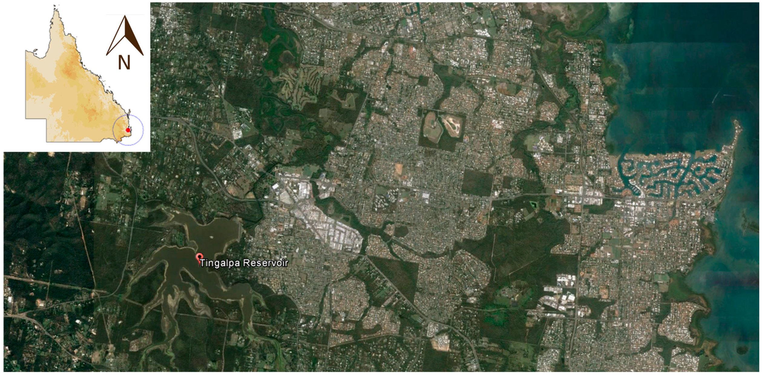
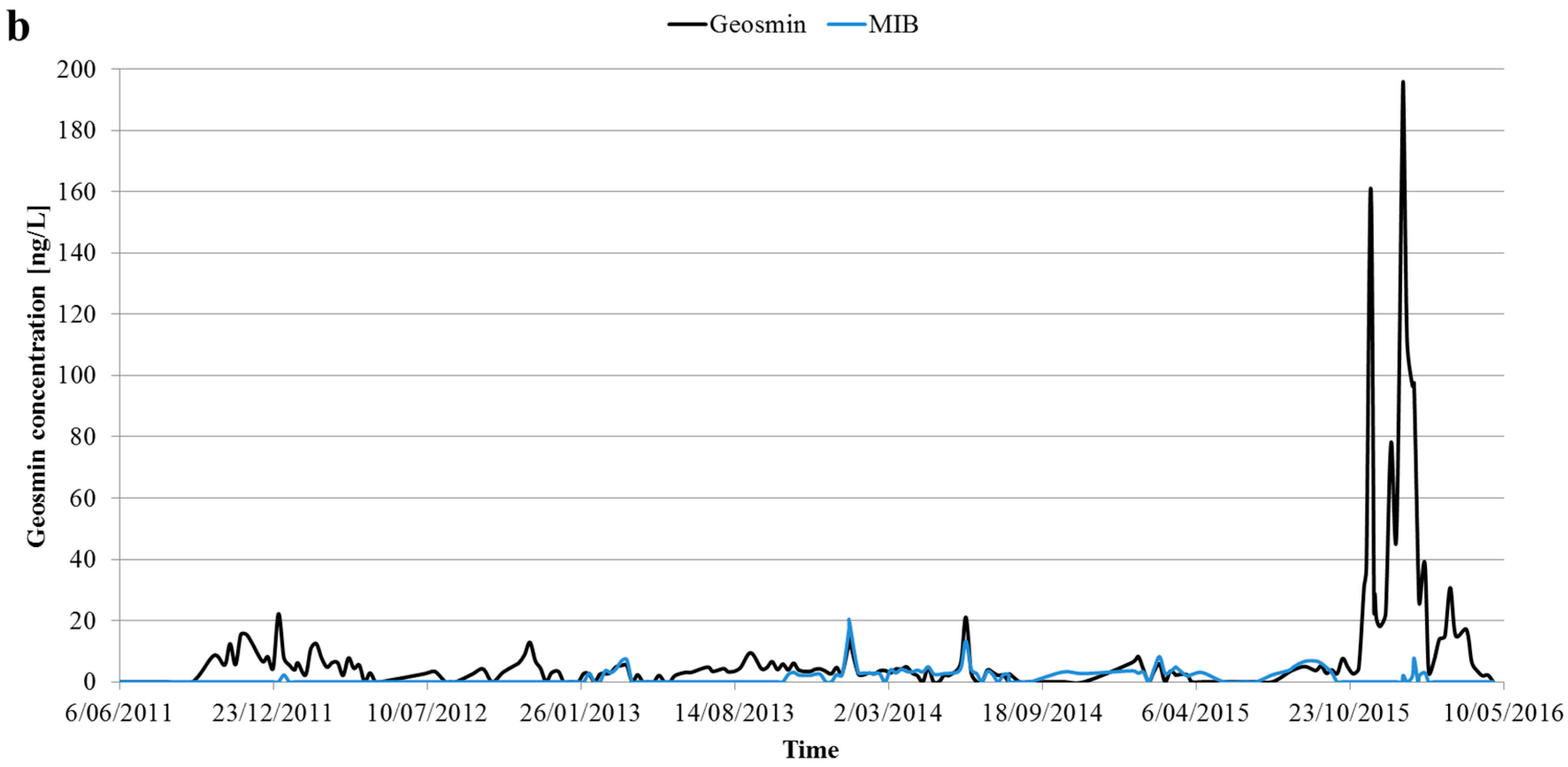
Figure 2 illustrates the temporal variation of sampled geosmin and MIB concentrations in the raw water of Lake Tingalpa since 2011.
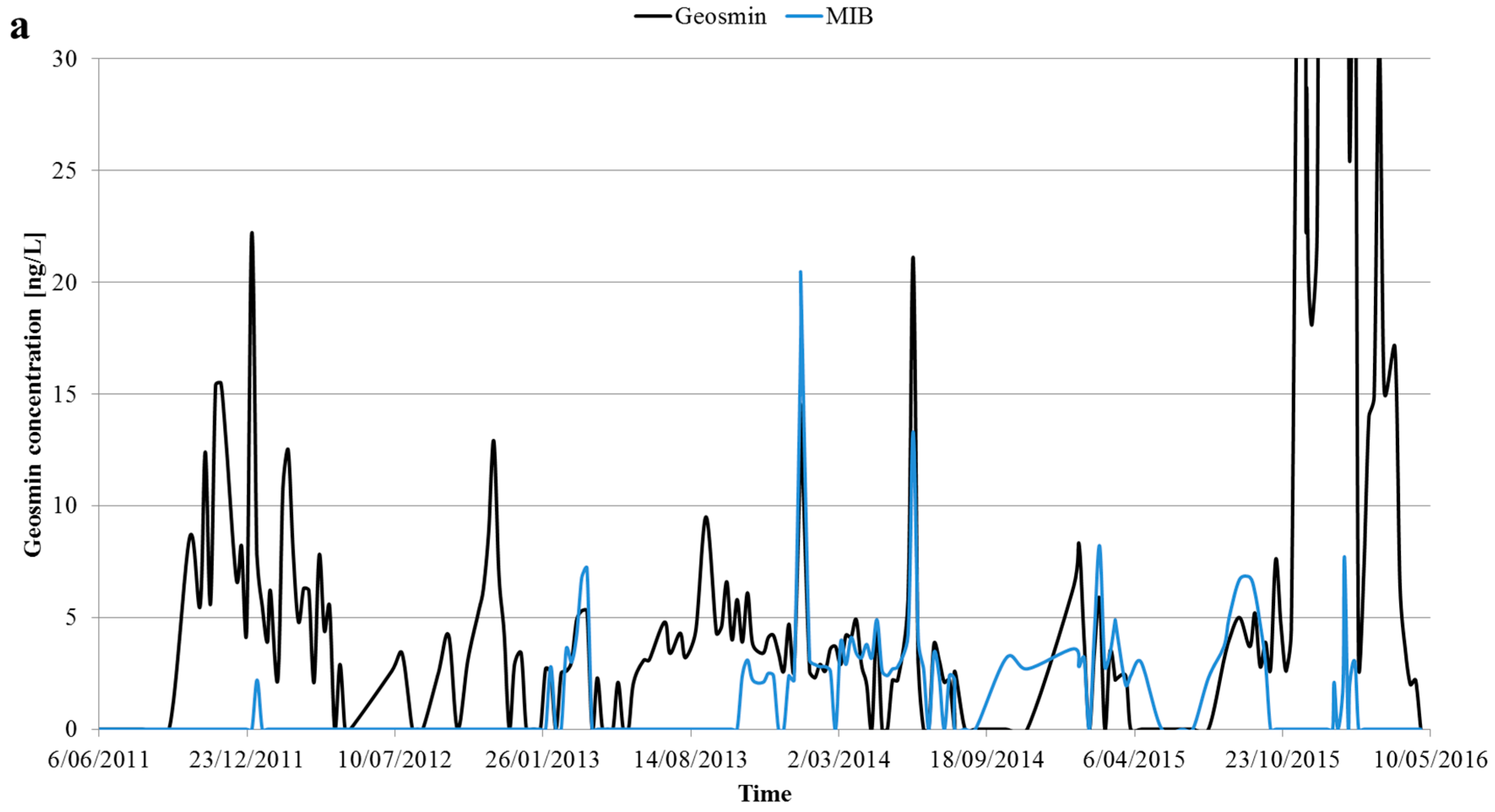
Figure 2a allows a better analysis of earlier, smaller events while
Figure 2b includes the major, more recent events. Therefore, it can be seen how a number of geosmin events above the detection threshold (5 to 10 ng/L) were detected over time, however two extreme events occurred during late spring/summer 2015, leading to concentrations over 150 ng/L, and resulting in wide spread customer complaints.
Table 1 displays how these events increased the calculated average geosmin concentrations. As a further consideration, MIB concentrations were consistently much lower than geosmin levels, thus the attention of this research shifted to geosmin only, after these preliminary outcomes.
As a first step, data were filtered to include only the events periods. Then, based on the literature and available data, a number of potential predictors were included, such as: total cyanophytes, as well as particular species of them (such as Microcystis aerug. and spp., Dolichospermum circ. and Merismopedia spp.), water temperature, reservoir volume, iron, total oxidised nitrogen, turbidity, and past week change in reservoir volume (proportional to rain and evaporation among others). Other parameters that were expected to play a role (such as dissolved oxygen and phosphorus) showed instead only a very weak correlation with geosmin peak events. Additionally, since geosmin was occasionally already detected the week/fortnight before the peak, the independent variable considered was the increase rate of geosmin, assumed linear, in ng/L per day, calculated by dividing the overall weekly/fortnightly variation by the number of days in between the two sampling (i.e., 7/14). This gives a better representation of the dynamics leading to the peak, and accounts for initial concentrations that might have been detected.
3.2. Self-Organising Maps
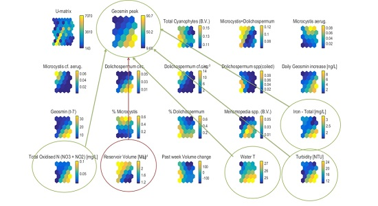
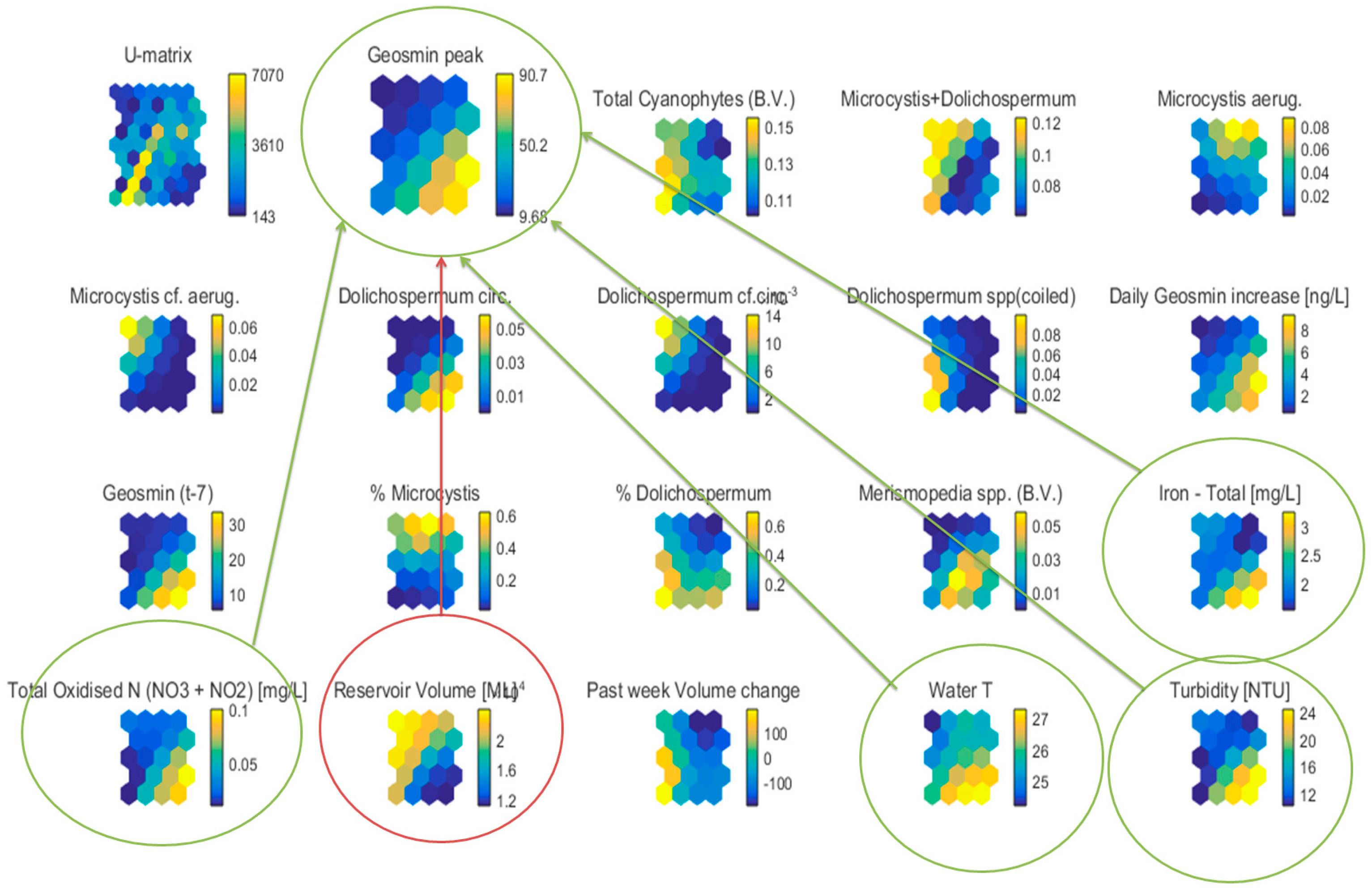
The prepared smaller dataset was used to create self-organising maps (
Figure 3).
Table 2 also presents the numerical quantification of each of these variables during those critical events, with conditional formatting helping to visually inspect similar trends. The first thing that can be noticed from the SOMs, is how the map for geosmin peaks has very similar colour patterns (highlighted with green connections) to turbidity, total iron, and total oxidised nitrogen (NO
3 and NO
2), as well as being inversely proportional to the reservoir volume (highlighted with a red connection). This means that any time there was a major geosmin peak, usually also those parameters recorded higher values; similarly, higher geosmin peak values were also recorded in times of low reservoir volume. From
Figure 4, a confirmation can be found and a very clear correlation can be seen between the substantial volume reduction, which occurred in winter 2014, and the sharp increases in iron, nitrogen and turbidity, most likely due to less dilution and increased reservoir instability leading to higher mixing. As a consequence, the geosmin peak events also became much more drastic. Increased nutrient availability is a well-documented factor cited in the literature that favours the production of geosmin. Turbidity was also found to positively correlate with geosmin in a number of studies [
9,
10]. Additionally, from the SOMs it can be also noticed how warmer water temperatures are typically linked to larger geosmin concentrations, as well as higher daily increase rates. This is again in agreement with the literature [
17,
19,
20], as it implies, for instance, a higher intracellular geosmin release.
3.3. Events Analysis
Table 2 allows for a better understanding of the role that cyanophytes blooms play in determining geosmin increment rates during peak events. The figure reports the biovolumes of total cyanophytes, as well as the sum of
Microcystis species and
Dolichospermum circ. (former
Anabaena), typically associated to T&O compounds production [
14,
28,
29]. This table also includes two entries (3 May 2012, and 14 October 2014) where, despite cyanophytes blooms, there was no detection of geosmin. In this way it was possible to gain a fuller picture of the relationships between cyanobacteria and geosmin events. In addition, for event extremely high algal counts, including cyanophytes, were recorded on 9 January 2014. Extremely high iron levels were also recorded. This event is not herein analysed or reported, since further investigation is required for this particular event, as the levels are incredibly high and sampling/analysis issues would need to be validated. As a confirmation, the sampling immediately preceding and following this critical one yielded values for all the parameters within absolutely normal ranges. Additionally, no geosmin was detected. Thus, given the uncertainty around it, this particular event was excluded from the next steps of the analysis.
Firstly, attention was focused on the two blooms not leading to geosmin peaks. On the 14 October 2014, a total cyanophytes biovolume of 0.191 mm3/L, the second highest in the dataset, was recorded. However, no geosmin was detected in the nearest sampling. This can be explained by the fact that neither Microcystis nor Dolichospermum species were detected; the dominant species leading to that bloom was Merismopedia spp., which is not known to be able to produce geosmin. This would strongly suggest that the type of cyanobacteria causing the bloom provides a much more useful prediction of a potential T&O event than the total aggregate cyanobacteria count. Nevertheless, the second event not leading to a geosmin peak event occurred on the 3 May 2012 (0.271 mm3/L, the highest value in the dataset), and in this case it was largely (98%) due to Microcystis and Dolichospermum circ. What is evident here, besides a high volume, is the low temperature of the raw water (22.5 °C). Although more research is needed, since contrasting outcomes emerged on the role of temperature in geosmin production, we can assume that below certain temperature thresholds, the production/release of geosmin by Microcystis species and Dolichospermum circ. is limited or inhibited. This also highlights how algal (cyanobacterial) blooms, despite often being a critical predictor for geosmin events, are only one of the factors of a far more complex system, where nutrients, dam level, temperature, and other parameters also play determinant roles.
3.4. Model Development
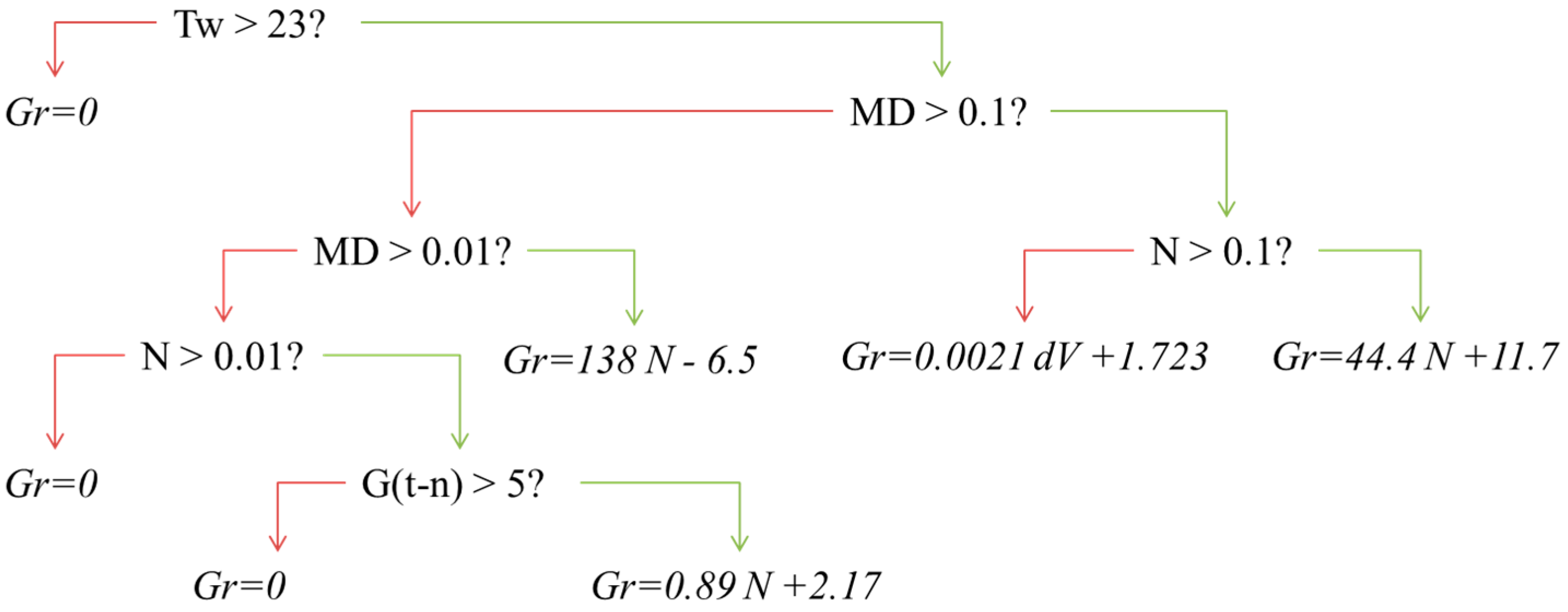
Based on the available data, its analysis and on the considerations above, we developed a conceptual regression tree, illustrated in
Figure 5. Since it is based on only few events, currently it cannot be deemed reliable to correctly estimate the exact amount of future peaks in geosmin. However, based on the analysis of historical events, it provides a structural hypothesis of relevant variables and processes, which determined the previous events or unexpected low values. Often, simpler regression models can outperform more complicated ones [
30]. It can be seen how variables, such as water temperature and total amount of geosmin-producing cyanophytes, do not directly enter the regression equation (i.e., their value is not directly proportional to the geosmin daily increase rate), however they are determinant factors in setting up thresholds under/above which different processes are inhibited or supported. Additionally, certain variables, such as iron, turbidity and reservoir volume, were not included in the model due to multicollinearity (i.e., they exhibit a similar behaviour to nitrogen), although they are relevant predictors too.
The first cut is set by water temperature; regardless of other factors, there is no evidence of geosmin events when the raw water temperature was below 23 °C. If the raw water is instead warmer than 23 °C, a number of other options are possible. Under this initial constraint, the presence of geosmin-producing cyanophytes plays a critical role. If they are not detected, and also nitrogen is not present, then there would be no increase whatsoever in geosmin concentration. Even if oxidised nitrogen is detected, geosmin might slightly increase only if it was already present in some noticeable (>5 ng/L) amounts in the previous sample. This can be due to the occurrence of a long peak event, which can persist if enough nutrients are available. If instead the geosmin-producing cyanophytes are detected, and in large amounts (i.e., >0.1 mm
3/L), then the rate of increase will depend on the available amount of nutrients (represented by oxidised nitrogen); if oxidised nitrogen is also present in large amounts (i.e., >0.1 mg/L), then the geosmin increase rate will be proportional to it; if instead, despite a bloom of geosmin-producing algae, there is no large amount of nutrients available, then the rate of increase would depend on the dam volume variation over the last week. In case of positive variation, rain and inflow were larger than evaporation and outflow, leading to higher increases in geosmin, which is in line with outcomes of previous studies [
11]. The remaining scenario is given by medium-size geosmin-producing algal blooms (i.e., between 0.01 and 0.1 mm
3/L); in this case, nitrogen plays again a critical role and its amount is proportional to the increase rate of geosmin.
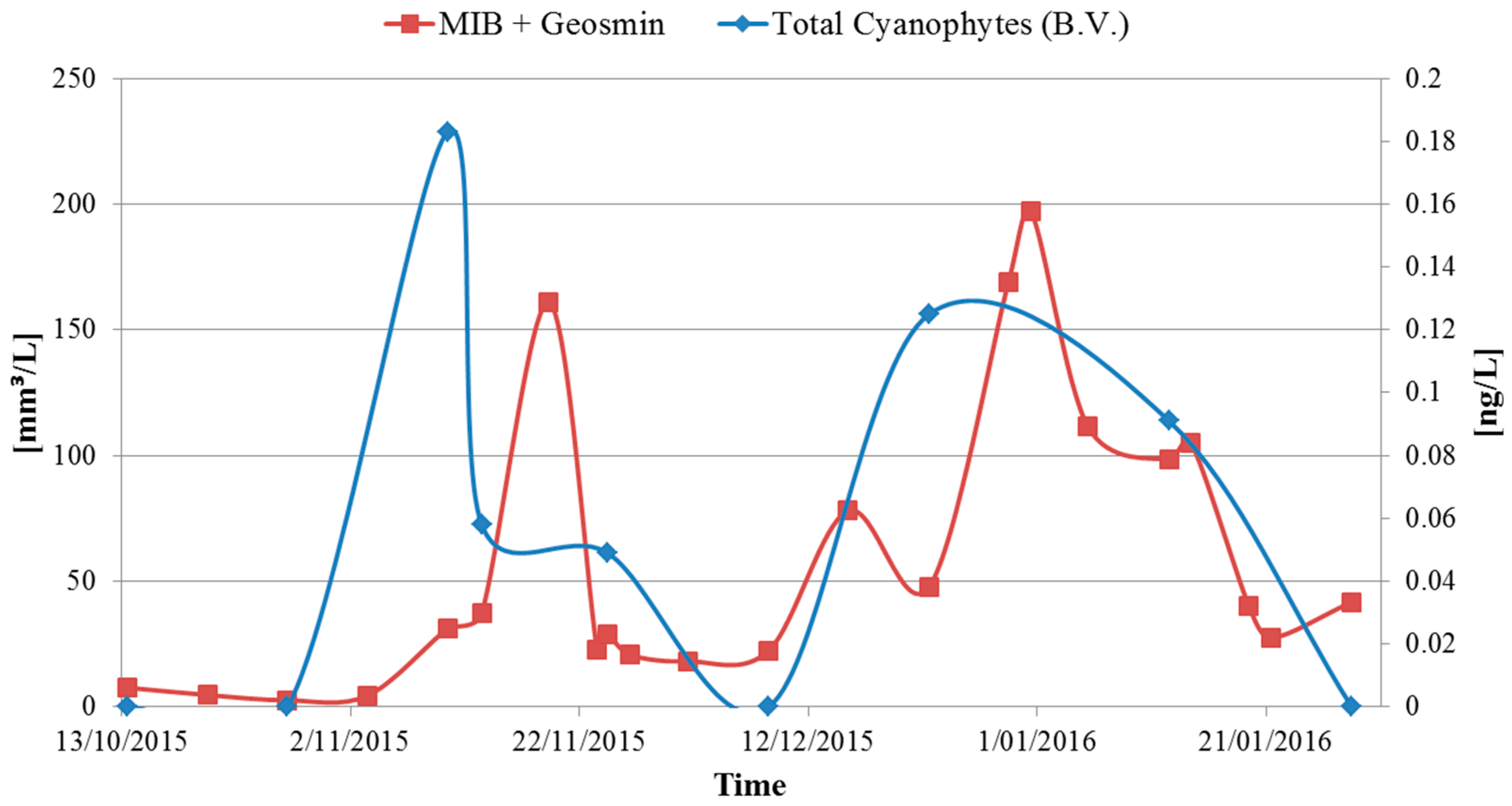
In order to validate the model, we focused on the two extreme events occurring at the end of 2015.
Figure 6 shows how both geosmin events were preceded by earlier peaks in total cyanophytes.
In addition,
Figure 7 shows the speciation of the cyanophytes. It can be seen how both peaks were largely caused by species of
Microcystis and
Dolichospermum, although the two peaks were quite different to each other. Looking back at
Figure 2, it seems that
Dolichospermum is responsible for the production of some MIB as well. However, as previously mentioned, the dominant compound is geosmin and this is produced by both
Microcystis and
Dolichospermum species.
Looking at the regression analysis tree developed in
Figure 5, the temperature detected in the raw water during that period (which corresponds to late spring and summer months) was consistently above the threshold of 23 °C, thus allowing for geosmin event to occur. Additionally, as it can be seen from
Figure 8, the total biovolume of
Microcystis and
Dolichospermum is above 0.1 mm
3/L, thus leading towards the far right side of the tree. Finally, it was pointed out (
Figure 4c) that the nutrient availability, in particular oxidised nitrogen, increased remarkably after the decrease in volume, reaching concentrations higher than 0.1 mg/L in the weeks preceding the geosmin event. Thus, these conditions led the developed model to predict sharp increases in geosmin levels; which actually occurred.
Since the peaks in relevant cyanophytes typically occur a couple of weeks before the T&O events, it is possible to use these data, as well as the other information (water temperature, oxidised nitrogen, dam volume variation) required by the tree, to estimate the potential for the occurrence of geosmin peak events, and thus proactively adjust the treatment procedures accordingly.
3.5. VPS Data Analysis and Predictive Potential
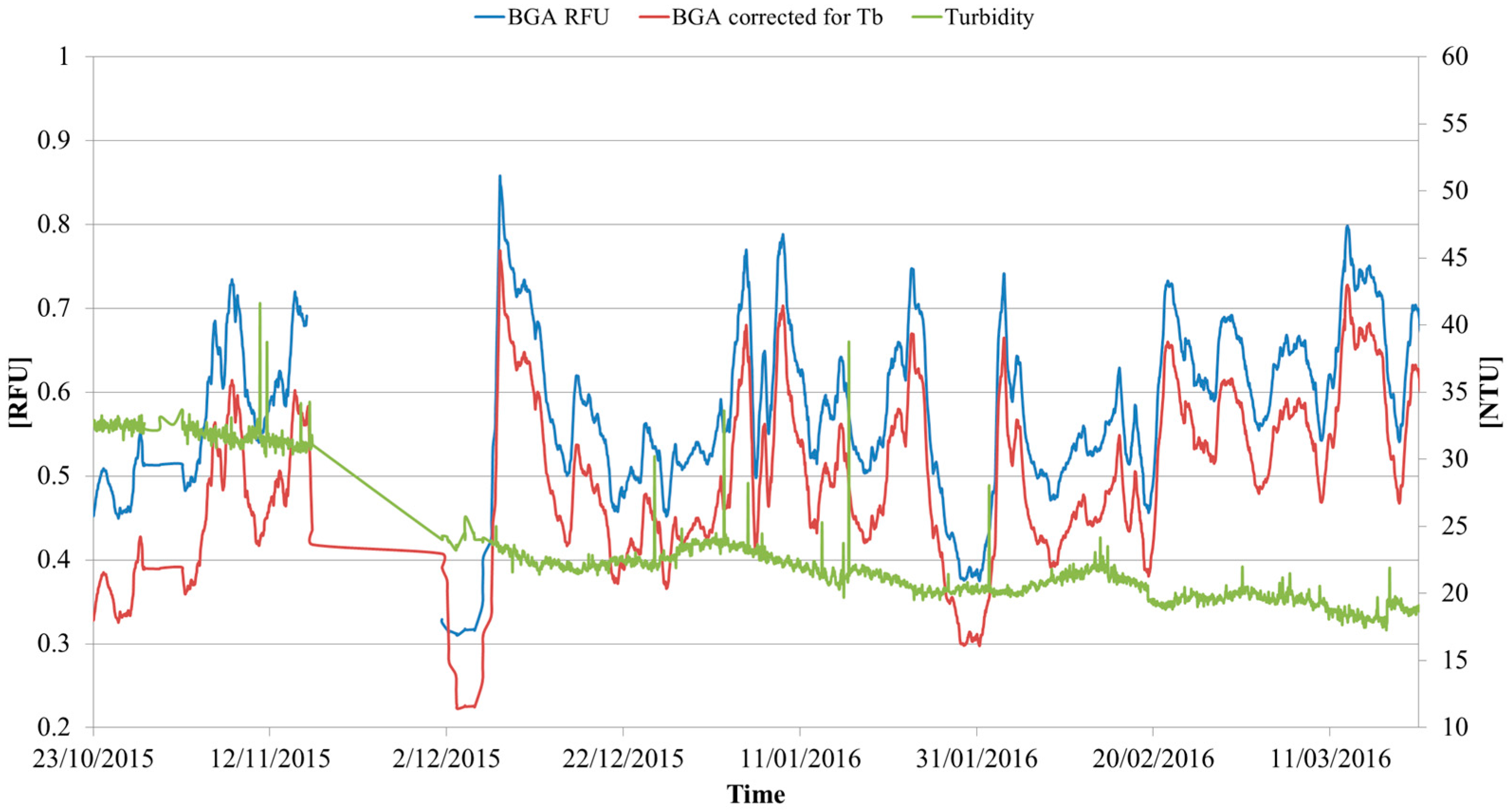
The historical data from the Vertical Profiling System (VPS) installed in Lake Tingalpa were analysed. The VPS was installed in 2013; hence it was possible to use its data for analysis of the more recent T&O events only. Additionally, during winter 2014, a number of sondes where changed from the previous YSI 6-Series Sensors to the newer EXO multiparameter water quality sonde product line, leading to newer units of measure, probe sensitivity to other water parameters and calibration procedures. Hence, for this study, we will focus on the two large 2015 events only. In particular, the aim was to analyse the phycocyanin-based blue-green algae (BGA-PC) sensor to see if it can be used to assist in predicting geosmin peak events.
The sensor measures blue-green algae in real-time through the in vivo fluorometry technique, which directly detects the fluorescence of a specific pigment in living algal cells and determines relative algal biomass. However, the sensor can be sensitive to variables such as turbidity, with newer EXO sondes less sensitive than the previous 6-series [
31]. In
Figure 8, the BGA readings (at depth = 1 m) adjusted for turbidity based on YSI indications [
31] are reported. A proper calibration should be performed for this specific location, which evaluate the effect of not only turbidity, but also of other variables; however this was out of the scope of this work. Although hourly data was provided, the chart shows 24-h moving averages. Between 16 November 2015, and 2 December 2015, the VPS was not operational and therefore data is missing for those two weeks. It can be noticed how, before 16 November 2015, the average turbidity was slightly higher (around 30 NTU) than in the following months (around 20 NTU), thus, by adjusting the readings, the difference in the BGA peak values in November and in December is relatively smaller than initially measured. Nevertheless the difference is minimal, and such adjustment would be crucial only in case of extreme turbidity events.
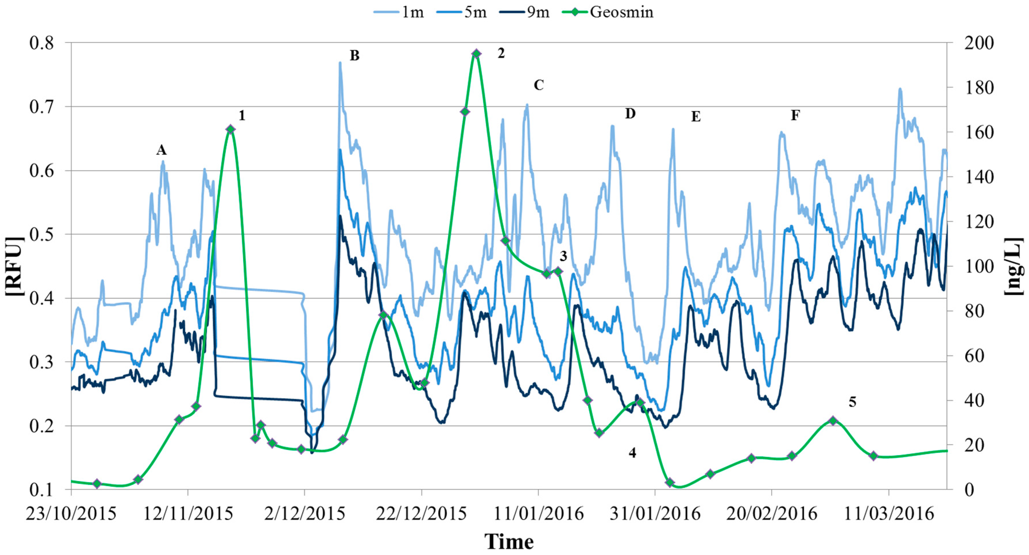
Figure 9 illustrates the BGA values at 1, 5 and 9 m depths of Lake Tingalpa, as well as the geosmin values in the raw water redirected to the Capalaba WTP. Typically, the values closer to the surface are higher than at the bottom, consistent with the literature findings (e.g., more light, higher temperatures, etc.). Although not extremely clear, a pattern can be noticed, with BGA peaks often anticipating geosmin high values. For instance, peak A in BGA occurred 12 days before the peak 1 in geosmin. Peak 2 occurred 23 days after a very high peak (B) in BGA; despite the longer lag, a smaller peak in geosmin was already detected 7 days later. Peak C also occurred 5 days before peak 3, as well as peak D with peak 4. Peak 5, interestingly, did not yield any sharp, lagged geosmin peak, although there was a slow, constant increase after that. Finally, peak F anticipated peak 5 by 8 days.
It is clear from the previous paragraphs how there is high complexity and uncertainty involved in these T&O events, and other parameters (e.g., water temperature, nitrogen, dam level) are as important as cyanobacteria. Nevertheless, given the large amount of VPS data which are collected remotely (i.e., no need for samplers), and in real-time, collected in the reservoir, future work (e.g., accurate calibration with manual sampling data; analysis of new events) could focus on better exploring the potential of the VPS BGA probe to be used as an input for a prediction model which could provide early warnings of T&O events. Although it was evident that also the strain of cyanophytes is a critical predictor, more work is needed to understand if the fluorescence approach of the BGA probe allows for all the strains to be detected, or not. The correlations found between its readings and T&O events are interesting as they may imply that the BGA probe can mainly detect T&O-causing strains. Additionally, similar VPS-based models were already developed by the authors [
30] for other parameters, leading to monetary and operational benefits for the water utility.
4. Conclusions
A comprehensive analysis of data related to a number of T&O events was performed for Lake Tingalpa and the Capalaba WTP. Geosmin was found to be the dominant compound, and two extremely high peaks occurred in November/December 2015. One of the key-factors triggering geosmin events was the occurrence of cyanobacteria blooms; however, the species of cyanobacteria was also a critical factor, since some of them (e.g., Merismopedia spp.) did not produce geosmin. Importantly, blooms alone cannot fully explain the occurrence and magnitude of geosmin events; other factors such as water temperature, nitrogen and reservoir volume variations were found to be determinant input factors. In particular, it was noticed how higher geosmin peaks have been recorded since the reservoir volume was lowered in 2014, and in turn turbidity and nutrients increased. As a result, a simple regression analysis tree was developed and validated to provide predictive capabilities and better understanding of geosmin peak events. Although such model can be already used, with caution, by the plant operators for early prediction of T&O events, this requires manual data input based on the results of the latest lake sampling; nevertheless, analysis of VPS BGA probe data, in conjunction with other VPS data (e.g., water temperature, turbidity), showed potential to use only remotely collected data to provide early warnings for T&O events. The development of such tool will be the focus of future research.


