
Relating Water Quality and Age in Drinking Water Distribution Systems Using Self-Organising Maps

 ,
,  , ,
, ,
Abstract
:1. Introduction
2. Methods and Materials
2.1. Hypotheses on Factors Influencing Microbial Water Quality Data
“The number of bacteria enumerated at 20–22 °C provides some indication of (1) the amount of food substance available for bacterial nutrition and (2) the amount of soil, dust and other extraneous material that had gained access to the water. The HPC at 37 °C affords more information relating to potentially dangerous pollution, as the organisms developing at this temperature are chiefly those of soil, sewage, or intestinal origin. Their number, therefore, may be used as an index of the degree of purity of the water” and “The ratio of the HPC at 22 °C to that at 37 °C is helpful in explaining sudden fluctuations, high ratios being associated with bacteria of clean soil or water saprophyte origin and, therefore, of ‘small significance’”.
2.2. Dutch Dataset
2.3. UK Datasets
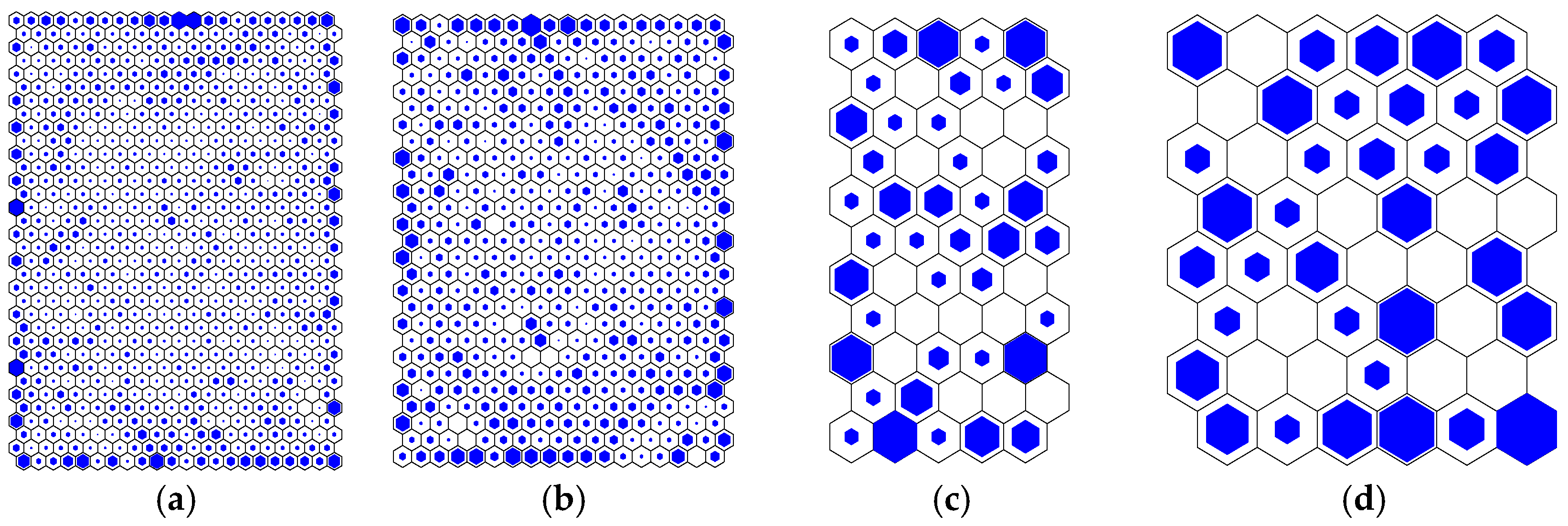
2.4. SOM Analysis
3. Results
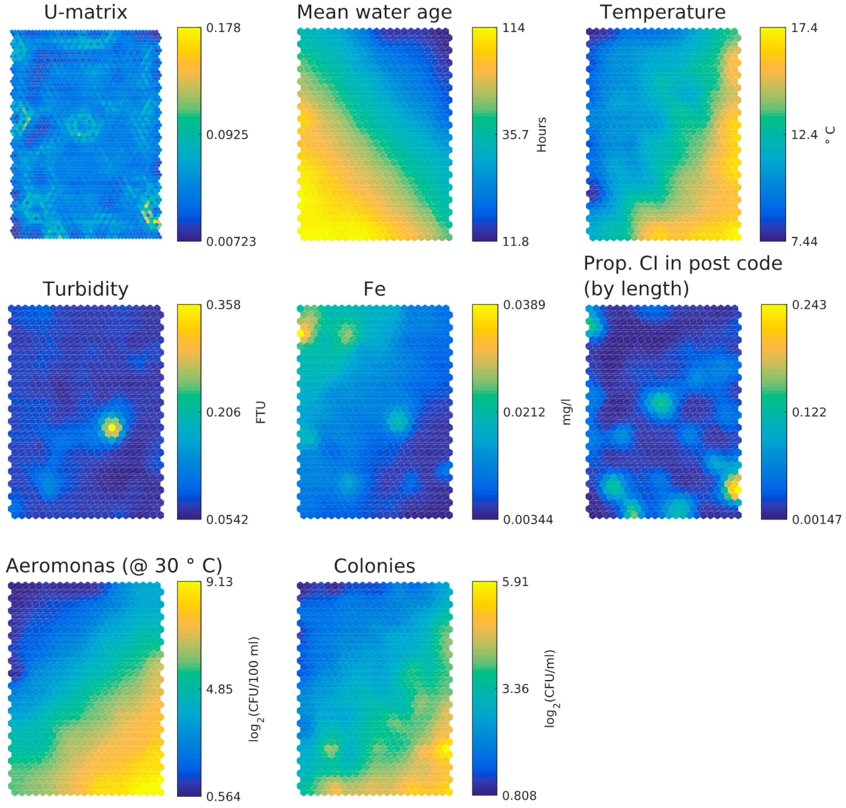
3.1. Dutch Dataset
- Water age and temperature are not correlated; this is as expected [3]
- Total iron and turbidity partly correlate; the highest turbidity values coincide with raised iron levels, presumably particulate iron, whereas the highest iron levels do not correlate with raised turbidity levels and this may indicate dissolved iron. Note that the values for iron and turbidity are all quite low. There seems to be a moderate correlation between higher iron levels and higher local cast iron percentage in the network.
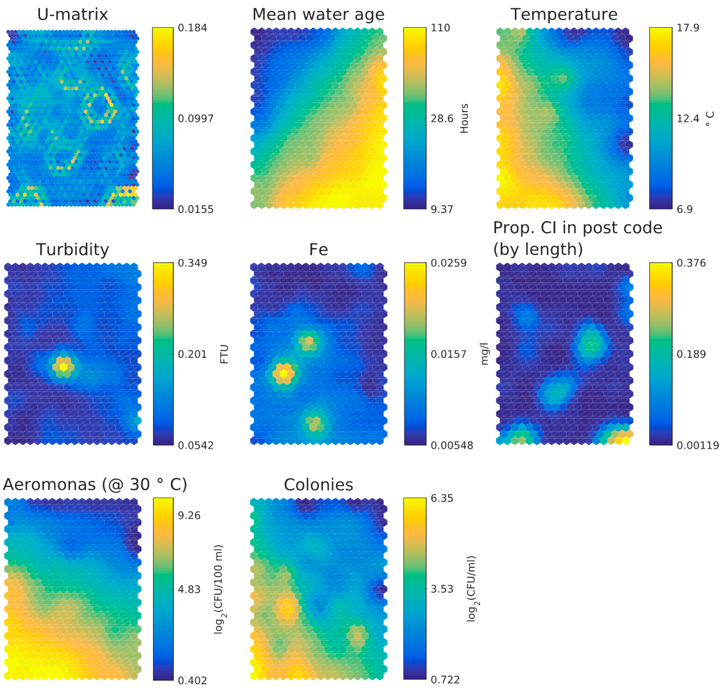
- HPC and Aeromonas correlate with each other and with temperature. There does not seem to be a correlation between Aeromonas and water age. Repeating the analysis segregated for the two main water sources (WTW Bergen and WTW Andijk) we see similar results, including a weak correlation between water age and Aeromonas for WTW Andijk (Figure 7 and Figure 5b).
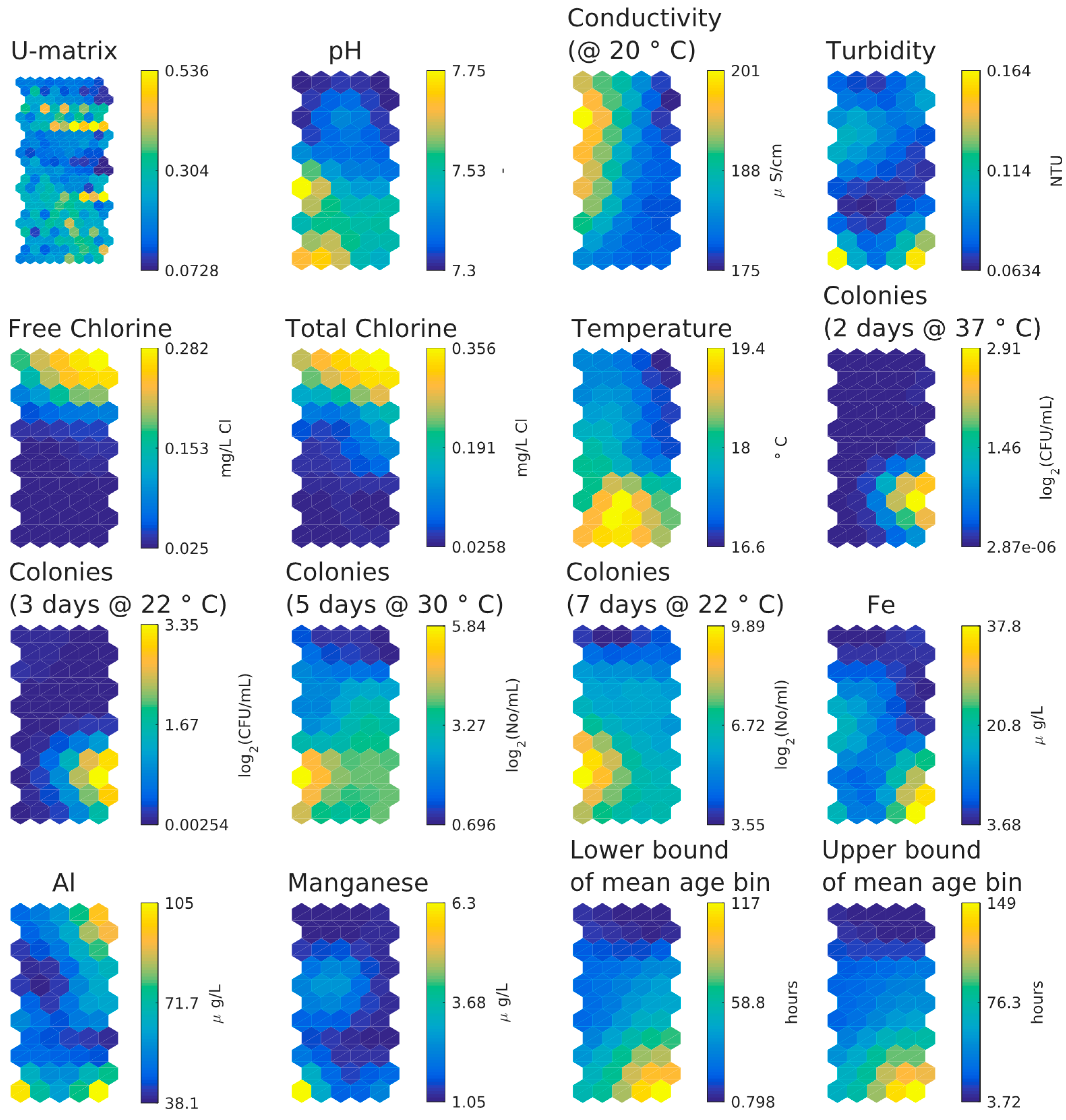
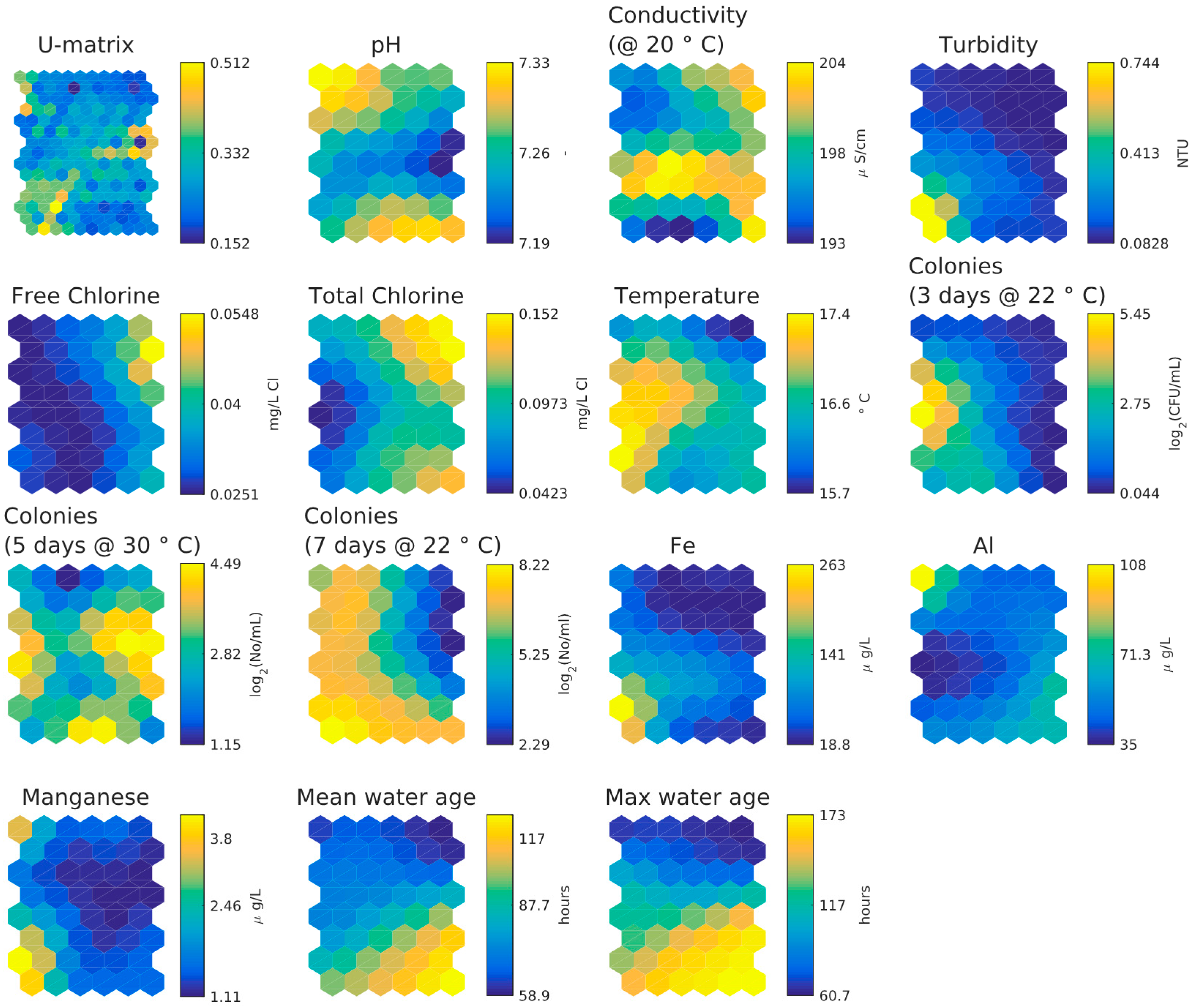
3.2. UK Customer Taps Dataset
- There is little difference between lower and upper bound of mean water age bin in SOM component plane plots.
- Inverse relationship between HPC and chlorine concentrations, strongest for the lower day HPC counts.
- Inverse relationship between chlorine and temperature/age.
- Weak relationship between age and temperature.
- Weak relationship between two days and three days HPC and age/temperature (HPC two days at 37 °C and three days at 22 °C strongly clustered).
- Weak relationship between five days and seven days HPC and age/temperature (HPC five days at 30 °C and seven days at 22 °C strongly clustered).
- Higher values of aluminium in the upper right-hand corner correlate with higher chlorine values and smaller water age values. Higher values of iron, aluminium and turbidity correlate in the lower right-hand corner but higher values of manganese, aluminium and turbidity correlate in the lower left-hand corner. Aluminium coagulant was used historically at the WTW and some of it entered the DWDS and some is found together with iron and manganese, in which case also a higher turbidity is found.
3.3. UK Small Looped Network Dataset
- Little difference between mean and max age bins in SOM component planes.
- Inverse relationship between chlorine concentration and three days HPC and weak inverse relationship between chlorine concentration and five days or seven days HPC.
- Temperature and water age appear to be independent.
- Five-day HPC features same higher values as three-day HPC plus some extra distinct higher values. This second cluster is possibly more representative of biofilm-associated microbial activity than bulk water activity.
- Five-day HPC and seven-day HPC are different.
- Higher values of iron, manganese and turbidity correlate in lower left-hand corner but higher values of manganese and aluminium correlate in upper left-hand corner (aluminium coagulant was used at the WTW and was historically suspected to be entering the DWDS as a result of filter breakthrough).
4. Discussion
5. Conclusions
Acknowledgments
Author Contributions
Conflicts of Interest
References
- US Environmental Protection Agency. Effects of Water Age on Distribution System Water Quality; EPA: Washington, DC, USA, 2002.
- Mounce, S.R.; Husband, S.P.; Furnass, W.R.; Boxall, J.B. Multivariate data mining for estimating the rate of discolouration material accumulation in drinking water distribution systems. IWA J. Hydroinform. 2016, 18, 96–114. [Google Scholar] [CrossRef]
- Blokker, E.J.M.; Pieterse-Quirijns, E.J. Modeling temperature in the drinking water distribution system. J. Am. Water Works Assoc. 2013, 105, E19–E29. [Google Scholar] [CrossRef]
- Blokker, E.J.M.; Vreeburg, J.; Speight, V. Residual chlorine in the extremities of the drinking water distribution system: The influence of stochastic water demands. In Proceedings of the 12th International Conference on Computing and Control for the Water Industry, Perugia, Italy, 20 February 2014.
- Havelaar, A.; Versteegh, J.; During, M. The presence of Aeromonas in drinking water supplies in the Netherlands. Int. J. Hyg. Environ. Med. 1990, 190, 236–256. [Google Scholar]
- Van der Kooij, D. Legionella in drinking-water suppliies. In Microbial Growth in Drinking-Water Supplies. Problems, Causes, Control and Research Needs; van der Kooij, D., van der Wielen, P.W.J.J., Eds.; IWA: London, UK, 2013; pp. 127–175. [Google Scholar]
- Machell, J.; Boxall, J. Field studies and modeling exploring mean and maximum water age association to water quality in a drinking water distribution network. J. Water Res. Plan. Manag. 2012, 138, 624–638. [Google Scholar] [CrossRef]
- Medema, G.J.; Smeets, P.W.M.H.; Van Blokker, E.J.M.; Lieverloo, J.H.M. Safe distribution without a disinfectant residual. In Microbial Growth in Drinking-Water Supplies. Problems, Causes, Control and Research Needs; van der Kooij, D., van der Wielen, P.W.J.J., Eds.; IWA: London, UK, 2013; pp. 95–125. [Google Scholar]
- Smeets, P.; Medema, G.; Van Dijk, J. The Dutch secret: How to provide safe drinking water without chlorine in the Netherlands. Drink. Water Eng. Sci. 2009, 2, 1–14. [Google Scholar] [CrossRef]
- Machell, J.; Smeets, P.W.M.H.; Van Blokker, E.J.M.; Lieverloo, J.H.M. Improved Representation of Water Age in Distribution Networks to Inform. Water Quality. J. Water Res. Plan. Manag. 2009, 135, 382–391. [Google Scholar] [CrossRef]
- Blokker, E.J.M.; Beverloo, H.; Vogelaar, A.J.; Vreeburg, J.H.G.; Van Dijk, J.C. A bottom-up approach of stochastic demand allocation in a hydraulic network model: A sensitivity study of model parameters. J. Hydroinform. 2011, 13, 714–728. [Google Scholar] [CrossRef]
- Mounce, S.R.; Sharpe, R.; Speight, V.; Holden, B.; Boxall, J. Knowledge discovery from Large disparate corporate databases using Self-Organizing Maps to help ensure supply of high quality potable water. In Proceedings of the 11th International Confernece on Hydroinformatics, New York, NY, USA, 17–21 August 2014.
- Machell, J.; Boxall, J. Modeling and Field Work to Investigate the Relationship between Age and Quality of Tap Water. J. Water Res. Plan. Manag. 2014, 140, 431–439. [Google Scholar]
- World Health Organization. Guidelines for Drinking-Water Quality: Recommendations; World Health Organization: Geneva, Switzerland, 2004; Volume 1. [Google Scholar]
- Standing Committee of Analysts. The assessment of taste, odour and related aesthetic problems in drinking waters. In Methods for the Examination of Waters and Associated Materials; Environmental Agency: London, UK, 1998. [Google Scholar]
- Standing Committee of Analysts. The microbiology of drinking water 2002—Part. I—The enumeration of heterotrophic bacteria by pour and spread plate techniques. In Methods for the Examination of Waters and Associated Materials; Environmanetal Agency: London, UK, 2002. [Google Scholar]
- Bartram, J.; Bartram, J.; Cotruvo, J.; Exner, M.; Fricker, C.; Glasmacher, A.; Bartram, J.; Cotruvo, J.; Exner, M.; Fricker, C.; et al. Heterotrophic Plate Counts and Drinking-Water Safety: The Significance of HPCs for Water Quality and Human Health; IWA Publishing: London, UK, 2003. [Google Scholar]
- Sartory, D.P. Heterotrophic plate count monitoring of treated drinking water in the UK: A useful operational tool. Int. J. Food Microbiol. 2004, 92, 297–306. [Google Scholar] [CrossRef] [PubMed]
- Liu, G.; Van der Mark, E.J.; Verberk, J.Q.J.C.; Van Dijk, J.C. Flow cytometry total cell counts: A field study assessing microbiological water quality and growth in unchlorinated drinking water distribution systems. BioMed Res. Int. 2013, 2013. [Google Scholar] [CrossRef] [PubMed]
- Geldreich, E.E. Microbial Quality of Water Supply in Distribution Systems; CRC Press: Boca Raton, Fl, USA, 1996. [Google Scholar]
- LeChevallier, M.W. Biofilms in drinking water distribution systems: Significance and control. In Identifying Future Drinking Water Contaminants; National Research Council: Washington, DC, USA, 1999; p. 206. [Google Scholar]
- Lehtola, M.J.; Michaela, L.; Miettinen, I.T.; Arja, H.; Terttu, V.; Martikainen, P.J. The effects of changing water flow velocity on the formation of biofilms and water quality in pilot distribution system consisting of copper or polyethylene pipes. Water Res. 2006, 40, 2151–2160. [Google Scholar] [CrossRef] [PubMed]
- LeChevallier, M.W.; Schulz, W.; Lee, R.G. Bacterial nutrients in drinking water. Appl. Environ. Microbiol. 1991, 57, 857–862. [Google Scholar] [PubMed]
- LeChevallier, M.W.; Welch, N.J.; Smith, D.B. Full-scale studies of factors related to coliform regrowth in drinking water. Appl. Environ. Microbiol. 1996, 62, 2201–2211. [Google Scholar] [PubMed]
- Van der Kooij, D. Assimilable organic carbon as an indicator of bacterial regrowth. J. Am. Water Works Assoc. 1992, 84, 57–65. [Google Scholar]
- Power, K.N.; Nagy, L.A. Relationship between bacterial regrowth and some physical and chemical parameters within Sydney's drinking water distribution system. Water Res. 1999, 33, 741–750. [Google Scholar] [CrossRef]
- Drinking Water Decree. 2015. Available online: http://wetten.overheid.nl/BWBR0030111/geldigheidsdatum_27-11-2015 (accessed on 27 November 2015).
- Van der Kooij, D.; Visser, A.; Hijnen, W. Growth of Aeromonas hydrophila at low concentrations of substrates added to tap water. Appl. Environ. Microbiol. 1980, 39, 1198–1204. [Google Scholar] [PubMed]
- Rouf, M.; Rigney, M.M. Growth temperatures and temperature characteristics of Aeromonas. Appl. Microbiol. 1971, 22, 503–506. [Google Scholar] [PubMed]
- Sekar, R.; Deines, P.; Machell, J.; Osborn, A.M.; Biggs, C.A.; Boxall, J.B. Bacterial water quality and network hydraulic characteristics: A field study of a small, looped water distribution system using culture-independent molecular methods. J. Appl. Microbiol. 2012, 112, 1220–1234. [Google Scholar] [CrossRef] [PubMed]
- Vatanen, T.; Osmala, M.; Raiko, T.; Lagus, K.; Sysi-Aho, M.; Orešič, M.; Honkela, T.; Lähdesmäki, H. Self-organization and missing values in SOM and GTM. Neurocomputing 2015, 147, 60–70. [Google Scholar] [CrossRef]
- Kalteh, A.M.; Hjorth, P.; Berndtsson, R. Review of the Self-Organizing Map (SOM) approach in water resources: Analysis, modelling and application. Environ. Model. Softw. 2008, 23, 835–845. [Google Scholar] [CrossRef]
- Astel, A.; Tsakovski, S.; Barbieri, P.; Simeonov, V. Comparison of self-organizing maps classification approach with cluster and principal components analysis for large environmental data sets. Water Res. 2007, 41, 4566–4578. [Google Scholar] [CrossRef] [PubMed]
- Mounce, S.; Douterelo, I.; Sharpe, R.; Boxall, J. A bio-hydroinformatics application of self-organizing map neural networks for assessing microbial and physico-chemical water quality in distribution systems. In Proceedings of the 10th International Conference on Hydroinformatics, Hamburg, Germany, 14–18 July 2012.
- Helsinki University of Technology. SOM Toolbox (for MATLAB) 2014. Available online: https://github.com/ilarinieminen/SOM-Toolbox/ (acccessed on 14 April 2016).
- Blokker, E.J.M.; Pieterse-Quirijns, E.J.; Vogelaar, A.; Sperber, V. Bacterial Growth Model in the Drinking Water Distribution System—An Early Warning System; KWR Watercycle Research Institute: Nieuwegein, The Netherlands, 2014; p. 31. [Google Scholar]


| Indicator | Description | Expected Correlation with Water Age | Expected Influence of Temperature | Dataset |
|---|---|---|---|---|
| Aeromonas (at 30 °C) | Grows in the sediments and biofilm | No direct correlation with water age, but may be indirectly through exchange with sediments and biofilm | Positive influence of temperature | Dutch |
| Spores of sulphite reducing Clostridia | Used as a process indicator for the treatment works in removal of pathogens No growth | No correlation with water age | No influence from temperature | Dutch |
| E. coli | Faecal indicator, does not grow in the DWDS | No correlation with water age | No influence from temperature | Dutch, UK |
| HPC at 37 °C (2 days) | Indicator of bacteria capable to grow at human body temperature | No growth in the DWDS, no correlation with water age | Optimum growth at high temperature, limited influence of temperature in DWDS | UK |
| HPC at 22 °C (3 days) | Indicator for bacteria in water that grow at 22 °C | Fast grower, possible correlation with water age | Could grow in the water, possible influence of temperature | Dutch, UK |
| HPC at 30 °C (5 days) | No growth in the DWDS, no correlation with water age | Optimum growth at high temperature, limited influence of temperature in DWDS | UK | |
| HPC at 22 °C (7 days) | Indicator for bacteria in water that grow at 22 °C | Slow grower, limited correlation with water age | Could grow in the water, possible influence of temperature | UK |
| Title | Unit | Number of Data Points | First Date | Last Date |
|---|---|---|---|---|
| Temperature | °C | 25,098 | 29 January 1997 | 2 March 2012 |
| Turbidity | FTU | 14,587 | 5 January 2004 | 30 September 2011 |
| Aeromonas | #cfu/100 mL | 14,577 | 3 July 1997 | 2 March 2012 |
| E. coli | #cfu/100 mL | 32,185 | 5 January 2004 | 30 September 2011 |
| HPC | #cfu/mL | 15,067 | 5 January 2004 | 30 September 2011 |
| Fe | mg/L | 15,440 | 6 April 2004 | 26 March 2013 |
| Spores of Clostridia | #cfu/100 mL | 6593 | 6 April 2004 | 30 September 2011 |
| Title | Unit | Not NaN | Non-NaN > 0 | Min | Max | ||
|---|---|---|---|---|---|---|---|
| Temperature | °C | 8763 | (37.9%) | 8763 | (100.0%) | 3.4 | 24.8 |
| Turbidity | FTU | 7286 | (31.6%) | 6592 | (90.5%) | 0.0 | 8.1 |
| Aeromonas | 2Log (#cfu)/100 mL | 6156 | (26.7%) | 4877 | (79.2%) | 0.0 | 11.0 |
| E. coli | 2LOG (#CFU)/100 mL | 12,855 | (55.7%) | 176 | (1.4%) | 0.0 | 9.7 |
| HPC | 2Log(#cfu)/mL | 7689 | (33.3%) | 6381 | (83.0%) | 0.0 | 14.3 |
| Fe | mg/L | 3076 | (13.3%) | 2769 | (90.0%) | 0.0 | 0.5 |
| Spores of Clostridia | #cfu/100 mL | 3856 | (16.7%) | 25 | (0.6%) | 0.0 | 2.6 |
| Water age | h | 23,092 | (100.0%) | 23,092 | (100%) | 6.1 | 330.5 |
| Percentage of Cast Iron | % | 22,955 | (99.4%) | 17,044 | (74.2%) | 0.0 | 75.0 |
| Parameter | Customer Taps | Small Looped Network | Of Interest? (After Preliminary Analysis) |
|---|---|---|---|
| pH | 7.2–8.1 | 7.1–7.5 | No, small variation |
| Conductivity | 170–215 | 180–220 | No, small variation (<10%) |
| Turbidity | <0.4 | <1.5 | Not likely, values are very low |
| free and total chlorine | 0.05–0.4 | <0.15 | Not for “small looped network”: values are too low to have any meaning |
| Temperature | 16–21 | 15–18 | No, small variation (for biological processes) |
| HPC at 37 °C for 2 days | Yes, if positive samples available | ||
| HPC at 22 °C for 3 days | Yes, if positive samples available | ||
| HPC at 30 °C for 5 days | Yes, if positive samples available | ||
| HPC at 22 °C for 7 days | Yes, if positive samples available | ||
| Fe | <50 | <200 | Yes |
| Al | <200 | <100 | Yes |
| Mn | <10 | <5 | Yes |
| water age lower and upper bound | 0–170 h | 60–170 h | Yes |
| Indicator | Expected Correlation with Water Age | Expected Influence from Temperature | Relation with Water Age Found | Relation with Temperature Found | |||
|---|---|---|---|---|---|---|---|
| Dutch Dataset | Customer Taps | Small Looped Network | Dutch Dataset | UK Datasets | |||
| Aeromonas | No direct correlation with water age | Positive influence of temperature | Yes, weak | N.A. | N.A. | Yes | N.A. |
| HPC at 37 °C (2 days) | No growth in the water, no correlation with water age | Optimum growth at high temperature, limited influence of temperature in DWDS | N.A. | Yes | N.A. | N.A. | N.A. |
| HPC at 22 °C (3 days) | Fast grower, correlation with water age | Could grow in the water, possible influence of temperature | Yes, weak | Yes | No | Yes | ? |
| HPC at 30 °C (5 days) | No growth in the water, no correlation with water age | Optimum growth at high temperature, limited influence of temperature in DWDS | N.A. | No | No | N.A. | ? |
| HPC at 22 °C (7 days) | Slow grower, limited correlation with water age | Could grow in the water, possible influence of temperature | N.A. | No | No | N.A. | ? |
© 2016 by the authors; licensee MDPI, Basel, Switzerland. This article is an open access article distributed under the terms and conditions of the Creative Commons by Attribution (CC-BY) license (http://creativecommons.org/licenses/by/4.0/).
Share and Cite
Blokker, E.J.M.; Furnass, W.R.; Machell, J.; Mounce, S.R.; Schaap, P.G.; Boxall, J.B. Relating Water Quality and Age in Drinking Water Distribution Systems Using Self-Organising Maps. Environments 2016, 3, 10. https://doi.org/10.3390/environments3020010
Blokker EJM, Furnass WR, Machell J, Mounce SR, Schaap PG, Boxall JB. Relating Water Quality and Age in Drinking Water Distribution Systems Using Self-Organising Maps. Environments. 2016; 3(2):10. https://doi.org/10.3390/environments3020010
Chicago/Turabian StyleBlokker, E.J. Mirjam, William R. Furnass, John Machell, Stephen R. Mounce, Peter G. Schaap, and Joby B. Boxall. 2016. "Relating Water Quality and Age in Drinking Water Distribution Systems Using Self-Organising Maps" Environments 3, no. 2: 10. https://doi.org/10.3390/environments3020010
APA StyleBlokker, E. J. M., Furnass, W. R., Machell, J., Mounce, S. R., Schaap, P. G., & Boxall, J. B. (2016). Relating Water Quality and Age in Drinking Water Distribution Systems Using Self-Organising Maps. Environments, 3(2), 10. https://doi.org/10.3390/environments3020010