
Structuring Nutrient Yields throughout Mississippi/Atchafalaya River Basin Using Machine Learning Approaches

1
Department of Natural Sciences, Southern University at New Orleans, New Orleans, LA 70126, USA
2
Department of Earth and Environmental Studies, Montclair State University, Montclair, NJ 07043, USA
3
Computational Science Initiative, Brookhaven National Laboratory, Upton, NY 11973, USA
*
Author to whom correspondence should be addressed.
Environments 2023, 10(9), 162; https://doi.org/10.3390/environments10090162
Submission received: 7 July 2023
/
Revised: 6 September 2023
/
Accepted: 14 September 2023
/
Published: 19 September 2023
Abstract
:To minimize the eutrophication pressure along the Gulf of Mexico or reduce the size of the hypoxic zone in the Gulf of Mexico, it is important to understand the underlying temporal and spatial variations and correlations in excess nutrient loads, which are strongly associated with the formation of hypoxia. This study’s objective was to reveal and visualize structures in high-dimensional datasets of nutrient yield distributions throughout the Mississippi/Atchafalaya River Basin (MARB). For this purpose, the annual mean nutrient concentrations were collected from thirty-three US Geological Survey (USGS) water stations scattered in the upper and lower MARB from 1996 to 2020. Eight surface water quality indicators were selected to make comparisons among water stations along the MARB over the past two decades. Principal component analysis (PCA) was used to comprehensively evaluate the nutrient yields across thirty-three USGS monitoring stations and identify the major contributing nutrient loads. The results showed that all samples could be analyzed using two main components, which accounted for 81.6% of the total variance. The PCA results showed that yields of orthophosphate (OP), silica (SI), nitrate–nitrites (NO3-NO2), and total suspended sediment (TSS) are major contributors to nutrient yields. It also showed that land-planted crops, density of population, domestic and industrial discharges, and precipitation are fundamental causes of excess nutrient loads in MARB. These factors are of great significance for the excess nutrient load management and pollution control of the Mississippi River. It was found that the average nutrient yields were stable within the sub-MARB area, but the large nitrogen yields in the upper MARB and the large phosphorus yields in the lower MARB were of great concern. t-distributed stochastic neighbor embedding (t-SNE) revealed interesting nonlinear and local structures in nutrient yield distributions. Clustering analysis (CA) showed the detailed development of similarities in the nutrient yield distribution. Moreover, PCA, t-SNE, and CA showed consistent clustering results. This study demonstrated that the integration of dimension reduction techniques, PCA, and t-SNE with CA techniques in machine learning are effective tools for the visualization of the structures of the correlations in high-dimensional datasets of nutrient yields and provide a comprehensive understanding of the correlations in the distributions of nutrient loads across the MARB.
1. Introduction
Numerous fish and wildlife species, including about 75% of waterfowl traversing the U.S., seabirds, wading birds, fur-bearers, and sport and commercial fisheries, are habituated in the Gulf’s coastal wetlands [1]. The Gulf of Mexico encompasses over five million acres (about half of the U.S. total). Unfortunately, hypoxia in the Gulf of Mexico threatens the coastal economy, and the water quality is decreased due to the increasing municipal and manufacturing needs, which are destroying coastal wetland habitats at an alarming rate [1]. The excess nutrients (N and P) in the Mississippi/Atchafalaya River Basin (MARB) are highly correlated with the hypoxic zone in the Gulf of Mexico [2]. To effectively manage and precisely control excess nutrient export from the MARB, it is important to understand the nature of nutrient loads, identify the critical source areas, and pinpoint the important sources of nutrients in specific areas [3,4].
Many efforts have been made to describe the major sources of N and P throughout the MARB and evaluate the effectiveness of nutrient reduction strategies [4]. Because of the randomness in the observations of nutrient loads [5], various statistical methods have been implemented to analyze trends in nutrient loads [6,7,8,9,10,11,12]. Linear regression was used to study yields throughout the MARB, considering various environmental impacts [13], and to identify the relative importance of sources and land use in nutrient delivery [14,15]. Forecasting methods, such as correlation, linear regression, principal component analysis (PCA), and clustering analysis (CA), are the most used statistical approaches for the analysis of water quality and spatial properties [16,17,18,19,20,21]. Spatially Referenced Regression on Watershed attributes (SPARROW) models and the Soil and Water Assessment Tool (SWAT) are the most commonly used simulation techniques to describe loads/yields throughout the MARB, analyze the relative importance of various sources, and evaluate the effectiveness of management practices [22,23,24,25]. Bayesian methods have been used in the decision analysis for environmental and resource management [26]. However, there is a defect in statistical methods such as linear regression and principal component analysis; that is, they can only capture global and linear variations in nutrient loads and are not able to analyze local and nonlinear variations in the distribution of nutrient loads. t-distributed stochastic neighbor embedding (t-SNE) is one of the promising machine learning methods to address this issue [27,28]. Moreover, there are few known studies combining the machine learning methods PCA, t-SNE, and CA to systematically analyze spatial properties in the distributions of nutrient loads throughout the MARB. This study investigates eight nutrient yields (ammonia nitrogen (NH3), dissolved organic carbon (DOC), nitrates–nitrites (NO3-NO2), orthophosphate (OP), silica (SI), total suspended sediment (TSS), total nitrogen (TN), and total phosphorus (TP)) throughout the MARB during 1996–2020 and explores the spatial properties of the distributions and variations in nutrient yields. The purpose of this research is to identify and visualize the structures in correlations of nutrient yield distribution and reveal the development of similarities in the nutrient yield distribution throughout the MARB using linear and nonlinear dimensionality reduction and clustering techniques, which may be useful to identify the critical source areas and pinpoint the important sources of nutrients in specific areas.
2. Materials and Methods
2.1. Materials
The surface water data used in this study were from the government public data source (https://www.sciencebase.gov/catalog/item/61c08ec5d34ee9cd54ed3425 (accessed on 22 May 2023), of which thirty-three water quality monitoring stations of the US Geological Survey (USGS) were selected. These stations were located in the states of Minnesota, Wisconsin, Iowa, Illinois, Missouri, Kentucky, Tennessee, Arkansas, Louisiana, and Mississippi, which are scattered in the upper, middle, and lower Mississippi/Atchafalaya River Basin (MARB), as shown in Figure 1 and Table 1. The water quality data were presented on an annual basis from 1996 to 2020 and recorded based on the water year (the 12-month period from October 1 for a given year through September 30 of the following year). The data contained eight basic nutrient yields, including ammonia nitrogen (NH3), dissolved organic carbon (DOC), nitrates–nitrites (NO3-NO2), orthophosphate (OP), silica (Si), total suspended sediment (TSS), total nitrogen (TN), and total phosphorus (TP), and they were used for a comprehensive evaluation of nutrient yields and the characterization of nutrient yields delivered from the MARB to the Gulf of Mexico.
2.2. Data Processing
The statistical software R 4.3.1 was employed to process and analyze the data collected at the water sampling stations. Data were cleaned up using Microsoft Excel and imported into the software R, and then the statistical results were obtained from R. A comparison among water quality data from different water stations was performed. Data on the nutrient yields used in statistical analysis are presented as the calculated average annual nutrient yields.
2.3. Principal Component Analysis (PCA)
Principal component analysis (PCA) is the machine learning method that can transform correlated variables into uncorrelated variables and evaluate the relative importance of correlated features. PCA is also one of the dimensionality reduction techniques [29]. To provide a comprehensive understanding involving all water quality parameters across the entire MARB, PCA was applied. The mathematical objective of PCA is to find a new set of orthogonal and uncorrelated variables or vectors , a linear combination of the original variables that can maximize the variance of original data or equivalently solve the constrained optimization problem
where the index i is the label of new variables and is covariance matrix where is the original data matrix and n represents the number of water monitoring stations. The solutions of vectors to the optimization problem are principal components, which are the directions of maximal variances of data. Thus, the original high-dimensional data can be analyzed in the lower-dimensional space spanned by vectors . The coefficients of the linear combination of the original variables from which the principal components (PCs) are constructed are called PCA loadings. The projections of original observations onto the principal components are called “scores” [29]. Kaiser–Meyer–Olkin [30] and Bartlett tests of sphericity [31] were used to evaluate the suitability of the data for PCA. All mathematical and statistical calculations were performed using the software R.
2.4. t-Distributed Stochastic Neighbor Embedding (t-SNE)
t-distributed stochastic neighbor embedding (t-SNE) is one of the dimension reduction machine learning techniques to visualize the structures of a high-dimensional dataset in a low-dimensional space. For a given set of n high-dimensional observations {}, the method of t-SNE aims to find corresponding representative points {} in low-dimensional space such that the statistical distance between the probability distribution in a high dimension, i.e., [27].
and the probability distribution in a low dimension, i.e.,
are minimized. The statistical distance is measured using Kullback–Leibler divergence [32]
2.5. Clustering Analysis (CA)
To understand the spatial structures of the distributions of nutrient yields across the MARB, clustering analysis was conducted. K-means clustering analysis identifies the latent behavior of a dataset by categorizing the observations into k groups or clusters on the basis of similarities [33]. The mathematical objective of K-means clustering is to find
where S is the k sets of {}, x is a set of observations {}, and is the mean of set . Hierarchical agglomerative clustering analysis is used to build a hierarchy of groups or clusters using an appropriate linkage criterion that specifies the dissimilarity of datasets as a function of the pairwise distances of observations in the datasets through a “bottom-up” approach [34].
3. Results
3.1. Distributions of Nutrient Yields (TN, TP, and SI)
The distribution of the average annual yields of total nitrogen, total phosphorus, and silica at thirty-three USGS water stations across the MARB are shown in boxplots in Figure 2, Figure 3 and Figure 4, respectively. As Figure 2 shows, there is a distinctly large nitrogen distribution group consisting of sites PROV, WAPE, KEOS, and VALL, with median yields ranging from 2.12 tons/square kilometer to 2.17 tons/square kilometer, while the remaining 29 have medians of around or less than 1.93 tons/square kilometer. Moreover, PROV, WAPE, and KEOS in Iowa and VALL in Illinois are located in the upper MARB along the Mississippi River. Iowa and Illinois are the heart of the Corn Belt, with the greatest amount of artificially drained soil, the highest percentage of total land in agriculture (corn and soybean), and the highest use of nitrogen fertilizers in the nation. From Figure 3, it can be seen that there is a distinct phosphorus distribution group consisting of the sites LELA, LONG, and MELV, which are located in the Lower Mississippi River Basin, with median yields ranging from 0.20 tons/square kilometer to 0.24 tons/square kilometer, while the remaining 30 have medians of less than 0.19 tons/square kilometer. Furthermore, the sites LELA and LONG are located in Mississippi, and MELV is in Louisiana. Mississippi produces more than half of the country’s farm-raised catfish, while agriculture and poultry products are the most important industries for Louisiana. This implies that these sites may be related to the emissions of surrounding industrial point sources [35,36]. The silica yields presented in Figure 4 show similar patterns in yield distribution as those of total phosphorus, presented in Figure 2.
3.2. PCA Results
In this study, PCA was conducted on eight nutrient yields for thirty-three USGS monitoring stations across the MARB. First, the applicability of PCA was tested using the Kaiser–Meyer–Olkin (KMO) and Barlett tests. These tests were used to verify the adequacy of the sample and the independence of each variable, respectively. The calculated results were KMO = 0.563 (>0.5) and the Barlett test’s significance (p < 0.001), indicating that the data were suitable for PCA.
3.2.1. Correlation Matrix
The correlation coefficient matrix was obtained using the R software, as shown in Table 2. From the table, it can be seen that OP, NH3, NO3-NO2, Si, DOC, TSS, TN, and TP showed a strong positive correlation (r > 0.7), which indicated that the variables were not independent and were suitable for PCA. TN, NO3-NO2, TP, and OP showed a significant positive correlation (r = 0.80~0.99). Furthermore, a significant relationship between TP and OP exists because OP is the principal form of dissolved P and contributes one-tenth to one-third of TP [13]. In addition, the significant correlation between OP and Si suggests that silicon availability may be related to phosphorus mobilization in soils [37].
3.2.2. Factor Loadings
Figure 5 is a scree plot that shows the eigenvalues or variances of each principal component (PC). The scree plot provided suggestions for an appropriate number of principal components chosen for study. It was observed that the slope became noticeably flatter after the second component. The first two principal components were preserved, which explained 81.6% of the variances in the dataset. Table 3 presents the loadings of the eight variables on PC1 and PC2. The first principal component (PC1), which explained 65.2% of the total variance, contained the largest negative loadings of OP (−0.40) and the second-largest negative loadings of TP (−0.39). The factor loadings of PC1 indicated that it mainly explains the phosphorus yielded primarily from manure, fertilizer, and municipal-point-source discharge across the MARB. The results indicate that phosphorus pollution is a major latent factor that influences water quality. The second principal component (PC2), explaining 16.4% of the total variance, is mainly an explanation of the variations in nutrient yields of NO3-NO2 (−0.57), TN (−0.47), and TSS (0.40). The factor loadings of PC2 implied that it explained the variation in nitrogen yields and suspended sediment. Furthermore, from the loadings of PC2, the effect of suspended sediment on the environment cannot be underestimated.
3.2.3. Factor Scores
A PCA biplot consisting of a score plot and a loading plot is shown in Figure 5. In Figure 5, each point represents a USGS water monitoring station. The axes show the principal components PC1 and PC2. The values on the axes represent the principal component scores of each monitoring station. The vectors are the loading vectors, whose components are in the magnitudes of the loadings in Table 3. From Figure 6, it can be seen that all eight variables are positively correlated, which is consistent with the correlation matrix and monitoring sites forming the groups based on annual yields. Furthermore, OP and SI are strongly correlated, and TP, DOC, and NH3 are highly associated. From the distribution of sites, it seemed that monitoring sites formed the groups based on similar annual yields. Although Nebraska’s site, ELKH, and Indiana’s site, CANN, are geologically separated, they formed a group for which their nutrient yields were negatively correlated with PC1 and positively correlated with PC2, and the scores are very similar. Kansas’s SEDG, Kentucky’s PADU, Iowa’s CLIN, and Minnesota’s HAST formed another group in which nutrient yields were positively correlated with both PC1 and PC2. Nebraska’s THED, Colorado’s DENV, and Missouri’s HERM formed a group with a positive association with PC1 and a negative association with PC2. The similarity among the sites may be related to similar percentages of cropland, geological features, urbanization, and precipitation [38]. In addition, from the relation between the site distribution and loading vectors, it can be seen that Mississippi’s LELA is aligned with TP, which means that Mississippi’s LELA has the largest TP yield, while Nebraska’s NICK has the largest TSS yield. The principal component scores of each USGS gauging station are listed in Table 4.
3.3. t-SNE Results
Figure 7 shows the results of applying t-SNE to the nutrient yields from 33 USGS monitoring sites across the MARB. The high-dimensional probability distribution is the Gaussian distribution, and the low-dimensional probability is Student’s t-distribution with one degree of freedom. All the nutrient yields of the 33 stations were used to compute the high-dimensional pairwise affinities pj|i. In implementation, the neighborhood graph was constructed using a conventional value of the effective number of k = 5 (~) nearest neighbors [27]. Figure 7 shows the consistent clustering results of the Figure 5 PCA biplot, in which the colors represent the labels of the monitoring sites. On the t-SNE map, the sites are seemingly separated into six clusters, and Louisiana’s MELV, Mississippi’s LELA, and Nebraska’s ELKH and NICK form a small, separate cluster. MELV and LELA are located in the lower MARB, while ELKH and NICK are in the upper MARB beside the Missouri River. The similarity in nutrient yields may be related to their major farming industries. In addition, Illinois’s GRAN and VALL, Missouri’s HERM, Indiana’s NEWH, HAZL, and CANN, Iowa’s WAPE and KEOS, and Kansas’s SEDG form a large cluster in which SEDG is located in a mountain–prairie area in the west of the middle MARB, while the rest of the sites are in the midwestern MARB and in the Corn Belt, with similar agricultural activities [38]. Furthermore, Nebraska’s THED, OMAH, and LOUI, Kansas’s DESO, Illinois’s THEB and GRAN, Montana’s SIDN, and Louisiana’s BELL and SIFR form another large cluster. This similarity may be related to their similar geological locations; that is, all these sites are distributed along the Missouri, Illinois, Ohio, and Mississippi rivers. Moreover, t-SNE revealed the main dimension of variation within each class; that is, the manifold comprises several distinct segments corresponding to different local structures, and each segment exhibits a continuously, linearly two-dimensional manifold.
3.4. CA Results
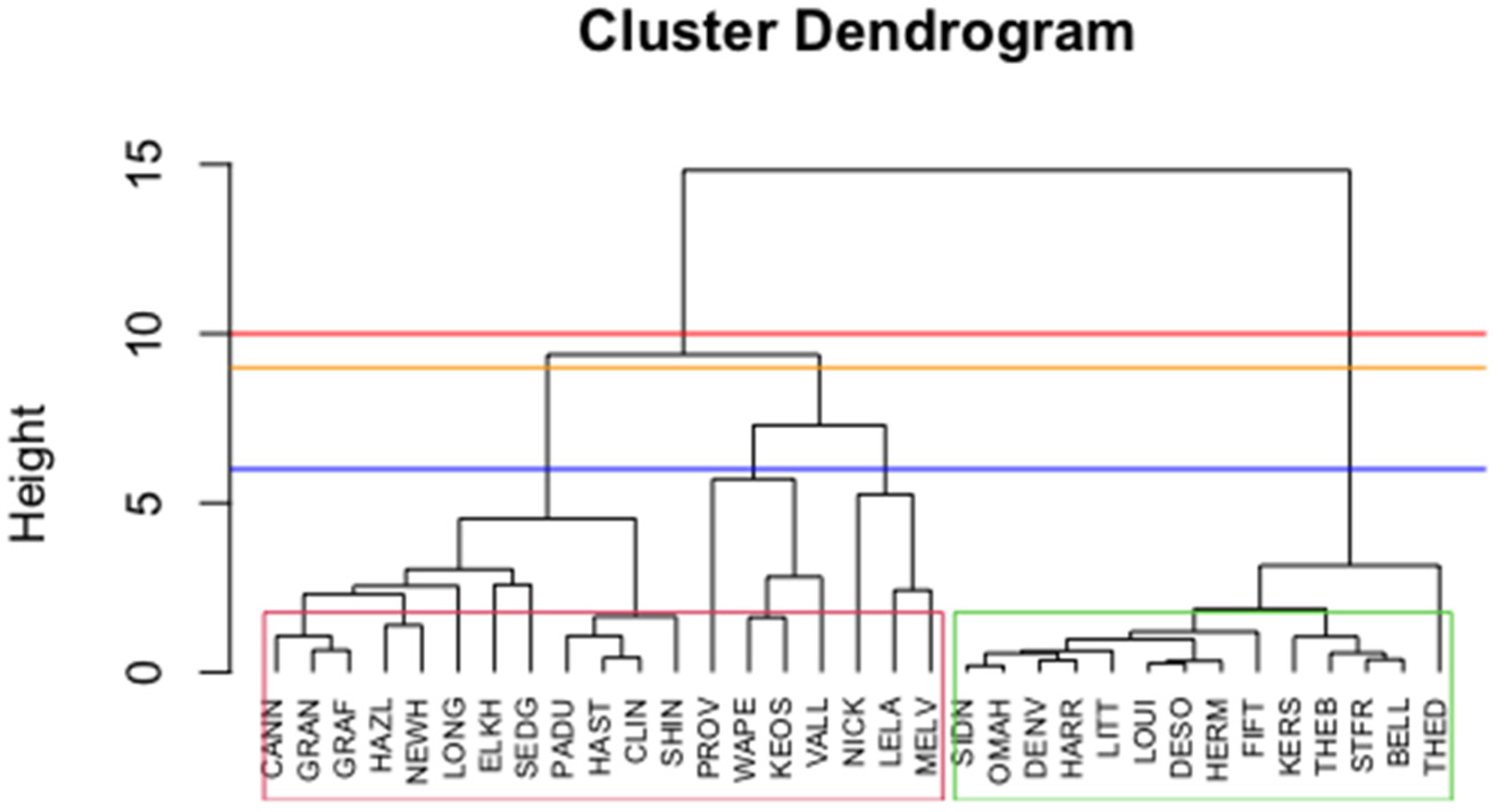
K-means cluster analysis (KCA) and hierarchical cluster analysis (HCA) were performed on the data, and the results are shown in Figure 8 and Figure 9, respectively. In KCA, the silhouette method was used to determine the optimal number of clusters by assessing the mean similarity within the cluster and mean dissimilarity between clusters. The metric for measuring the distance for the raw and centroid was Euclidean distance. From Figure 8, it can be seen that the sites are divided into five clusters: two large clusters and three small clusters. WAPE and KEOS, ELKH and CANN, and VALL and NEWH form the three small clusters. HAZL, GRAN, GRAF, CLIN, HAST, PADU, and SEDG and THED, HERM, THEB, STFR, BELL, SIDN, and SHIN form two large groups. In HCA, an agglomerative clustering algorithm was adopted, and Ward’s method was used to assess the similarity between each cluster by calculating the total sum of squared variations from the mean of a particular cluster and the proportion of variation explained by a particular clustering of the observations. As shown in Figure 9, HCA presented consistent results, as shown in PCA and KCA. In the nutrient yields from the 33 monitoring sites, 10 pair groups emerged. These sites are either located close to each other or along the same tributaries of the Mississippi River. Two large group sets have consistent elements, as shown in KCA.
4. Discussions
Louisiana’s MELV, Mississippi’s LELA, and Nebraska’s ELKH and NICK were found constantly to be assigned into the cluster that indicates suspended sediment accumulation. These sites have yields of DOC, NH3, NO3-NO2, OP, SI, TN, and TP around the mean values. However, these sites have TSS yields 141% greater than the mean values. MELV is located in Pointe Coupee Parish County, Louisiana. The parish’s economy is heavily reliant on agriculture, with sugar cane being one of the main cash crops. In 2010, the center of the population of Louisiana was located in Pointe Coupee Parish in the city of New Roads. Over 30,000 acres of Pointe Coupee Parish drain into the False River, and dirt has built up over time. LELA is located in Washington County, Mississippi. The Lake Washington watershed is in Washington County, near the Mississippi River in the Mississippi Delta, an area of the state that is very flat and has little to no relief for impairment caused by sedimentation. NICK is in Maple Creek, near Nickerson, Nebraska. The base flow at Maple Creek near Nickerson is shallow and slow, which leads to a buildup of sediment. ELKH is located on the Elkhorn River in Waterloo, Nebraska. It was reported that both the percentage of sand and the concentration of sand in the suspended sediment were much higher for the Platte and Elkhorn Rivers than for streams in the Big Blue River and Nemaha River basins. For Platte River at Louisville and for Elkhorn River at Waterloo, the measured sediment discharges ranged from about 7 to 94 percent of the computed total sediment discharge [39,40].
Illinois’s GRAN and VALL, Missouri’s HERM, Indiana’s NEWH, HAZL, and CANN, Iowa’s WAPE and KEOS, and Kansas’s SEDG form a large cluster indicating stretches of river with similar nutrient yields. Except for SEDG, all the other sites and their respective river locations comprise GRAN and CANN along the Ohio River, VALL along the Illinois River, HERM along the Missouri River, NEWH along the Wabash River, HAZL along the White River, WAPE along the Iowa River, and KEOS along the Des Moines River. The Wabash and White rivers are tributaries of the Ohio River, and the Ohio, Iowa, and Des Moines rivers are tributaries of the Mississippi River. It is important to notice that in this cluster, although SEDG is located in a mountain–prairie area, SEDG is located in Sedgwick County, which is the second-most-populous county in Kansas, with the presence of economic and industrial activities.
Nebraska’s THED, OMAH, and LOUI, Kansas’s DESO, Illinois’s THEB and GRAN, Montana’s SIDN, and Louisiana’s BELL and SIFR form another large cluster. This similarity may be related to their geological distribution and similar agricultural activities. DESO is located downstream of OMAH and LOUI. In addition, all these sites are distributed either along the Mississippi River or along its tributaries, indicating that nutrient yields are similar among these stretches of rivers [20]. THED is located along the Dismal River, OMAH along the Missouri River, LOUI along the Platte River, GRAN along the Ohio River, SIDN along the Yellowstone River, and THEB, BELL, and SIFR along the Mississippi River. The Yellowstone River is a tributary of the Missouri River and is considered the principal tributary of upper Missouri. The Platte River is a major river in the state of Nebraska and is also a tributary of the Missouri River. The Missouri River enters the Mississippi River north of St. Louis, Missouri. The Ohio River is a tributary of the Mississippi River and is located at the boundary of the midwestern and southern United States. The Ohio River enters the Mississippi River at the southern tip of Illinois.
5. Conclusions
In this study, the PCA, t-SNE, and CA methods were used to study the structures in the distribution of nutrient yields from the MARB to the Gulf of Mexico. This study analyzed the spatial characteristics of nutrient yields during 1996–2020 across the MARB. The PCA method was used to extract the most significant indicator parameters affecting the distribution of nutrient yields and to identify the possible pollution sources across the MARB. The temporal and spatial structures in the distribution of nutrient yields were visualized using the PCA, t-SNE, and CA methods. Eight nutrient yields were reduced to two important principal components using PCA, explaining 81.6% of the total variance of the original data set. PC1 (65.2%) represented orthophosphate- and silica-related nutrient yields, and PC2 (16.4%) represented nitrate–nitrite- and total-suspended-sediment-related nutrient yields. The management of nitrogen yields in the upper MARB and phosphorus yields in the lower MARB should be strengthened. With the effective treatment of industrial-point-source pollution, the impact of agricultural, rural non-point sources on tributary rivers and in stream channel erosion has gradually become prominent. However, sediment in the soil and stream bed cannot be ignored. This study comprehensively identified and visualized the structures and similarities in high-dimensional datasets on the distribution of nutrient yields across the MARB. The results of this study could arouse more rational attention to drive the improvement in the delicate management of nutrient loads from the MARB to the Gulf of Mexico. This study proved that the integration of dimension reduction techniques such as PCA and t-SNE with classification techniques such as CA in machine learning is an effective tool with which to identify and visualize the structures in high-dimensional datasets on nutrient yields and to provide a comprehensive understanding of the correlations of the distribution of nutrient loads across the MARB. Future works should consider more parameters, such as electrical conductivity, dissolved oxygen, the use of the landscape, hydrology, climate, and pH, to study variations in the temporal and spatial correlations of nutrient yield distribution.
Author Contributions
Study conceptualization, Y.Z., H.F. and S.Y.; data processing and modeling tasks, Y.Z., H.F. and S.Y.; analysis and result interpretation, Y.Z., H.F. and S.Y.; writing—original draft preparation, Y.Z.; writing—review and editing, H.F. and S.Y. All authors have read and agreed to the published version of the manuscript.
Funding
This research received no external funding.
Data Availability Statement
The data are publicly available on the USGS website (https://www.sciencebase.gov/catalog/item/61c08ec5d34ee9cd54ed3425, accessed on 6 July 2023).
Acknowledgments
We gratefully acknowledge the staff members at the Office of Education Programs and the Computational Science Initiative at Brookhaven National Laboratory for their support and assistance in this research. We also thank Data Chief Aub N. Ward and Data Scientist Daniel Kroes, Lower Mississippi Gulf Water Science Center, USGS, for their support and assistance in this research. This work was supported in part by the U.S. Department of Energy, Office of Science, Office of Workforce Development for Teachers and Scientists (WDTS), under the Visiting Faculty Program (VFP).
Conflicts of Interest
We declare that we do not have any commercial or associative interests that represent conflicts of interest in connection with the work submitted.
References
- McKinney, L.D.; Shepherd, J.G.; Wilson, C.A.; Hogarth, W.T.; Chanton, J.; Murawski, S.A.; Sandifer, P.A.; Sutton, T.; Yoskowitz, D.; Wowk, K.; et al. The Gulf of Mexico AN OVERVIEW. Oceanography 2021, 34, 30. [Google Scholar] [CrossRef]
- USEPA (U.S. Environmental Protection Agency). Nutrient Criteria Technical Guidance Manual—Lakes and Reservoirs; U.S. Environmental Protection Agency, Office of Water: Washington, DC, USA, 2000; 232p.
- Robertson, D.M.; Schwarz, G.E.; Saad, D.A.; Alexander, R.A. Incorporating Uncertainty into the Ranking of SPARROW Model Nutrient Yields from Mississippi/Atchafalaya River Basin Watersheds. J. Am. Water Resour. Assoc. 2009, 45, 534. [Google Scholar] [CrossRef]
- Robertson, D.M.; Saad, D.A. Nitrogen and Phosphorus Sources and Delivery from the Mississippi/Atchafalaya River Basin: An Update Using 2012 SPARROW Models. J. Am. Water Resour. Assoc. 2021, 57, 406. [Google Scholar] [CrossRef]
- LIoyd, C.E.M.; Freer, J.E.; Johnes, P.J.; Collins, A.L. Using hysteresis analysis of high-resolution water quality monitoring data, including uncertainty, to infer controls on nutrient and sediment transfer in catchments. Sci. Total Environ. 2016, 543, 388. [Google Scholar] [CrossRef]
- Morales-Marín, L.A.; Chun, K.P.; Wheater, H.S.; Lindenschmidt, K.E. Trend analysis of nutrient loadings in a large prairie catchment. Hydrol. Sci. J. 2017, 62, 657. [Google Scholar] [CrossRef]
- Feng, H.; Qian, Y.; Cochran, J.K.; Zhu, Q.; Hu, W.; Yan, H.; Li, L.; Huang, X.; Chu, Y.S.; Liu, H.; et al. Nanoscale measurement of trace element distributions in Spartina alterniflora root tissue during dormancy. Sci. Rep. 2017, 7, 40420. [Google Scholar] [CrossRef] [PubMed]
- Nie, J.; Mirza, S.; Viteritto, M.; Li, Y.; Witherell, B.B.; Deng, Y.; Yoo, S.; Feng, H. Estimation of nutrient (N and P) fluxes into Newark Bay, USA. Mar. Pollut. Bull. 2023, 190, 114832. [Google Scholar] [CrossRef] [PubMed]
- Antonopoulos, V.Z.; Papamichail, D.M.; Mitsiou, K.A. Statistical and trend analysis of water quality and quantity data for the Strymon River in Greece. Hydrol. Earth Syst. Sci. 2001, 5, 679. [Google Scholar] [CrossRef]
- Alexander, R.B.; Smith, R.A. Trends in the nutrient enrichment of U.S. rivers during the late 20th century and their relation to changes in probable stream trophic conditions. Limnol. Oceanogr. 2006, 51, 639. [Google Scholar] [CrossRef]
- Fernández del Castillo, A.; Yebra-Montes, C.; Verduzco Garibay, M.; de Anda, J.; Garcia-Gonzalez, A.; Gradilla-Hernández, M.S. Simple Prediction of an Ecosystem-Specifific Water Quality Index and the Water Quality Classifification of a Highly Polluted River through Supervised Machine Learning. Water 2022, 14, 1235. [Google Scholar] [CrossRef]
- Du, J.L.; Feng, H.; Nie, J.; Li, Y.; Witherell, B.B. Characterisation and assessment of spatiotemporal variations in nutrient concentrations and fluxes in an urban watershed: Passaic River Basin, New Jersey, USA. Int. J. Environ. Pollut. 2018, 63, 154. [Google Scholar] [CrossRef]
- Goolsby, D.A.; Battaglin, W.A.; Lawrence, G.B.; Artz, R.S.; Aulenbach, B.T.; Hooper, R.P.; Keeney, D.R.; Stensland, G.J. Flux and Sources of Nutrients in the Mississippi-Atchafalaya River Basin: Topic 3 Report for the Integrated Assessment on Hypoxia in the Gulf of Mexico; NOAA Coastal Ocean Program Decision Analysis Series No. 17; NOAA Coastal Ocean Program: Silver Spring, MD, USA, 1999; 130p.
- David, M.B.; Drinkwater, L.E.; McIssac, G.F. Sources of Nitrate Yields in the Mississippi River Basin. J. Environ. Qual. 2010, 39, 1657. [Google Scholar] [CrossRef] [PubMed]
- Jacobson, L.M.; David, M.B.; Drinkwater, L.E. A Spatial Analysis of Phosphorus in the Mississippi River Basin. J. Environ. Qual. 2011, 40, 931. [Google Scholar] [CrossRef] [PubMed]
- Feng, H.; Qian, Y.; Cochran, J.K.; Zhu, Q.; Heilbrun, C.; Li, L.; Hu, W.; Yan, H.; Huang, X.; Ge, M.; et al. Seasonal differences in trace element concentrations and distribution in Spartina alterniflora root tissue. Chemosphere 2018, 204, 359. [Google Scholar] [CrossRef] [PubMed]
- Schreiber, S.G.; Schreiber, S.; Tanna, R.N.; Roberts, D.R.; Arciszewski, T.J. Statistical tools for water quality assessment and monitoring in river ecosystems—A scoping review and recommendations for data analysis. Water Qual. Res. J. 2022, 57, 40. [Google Scholar] [CrossRef]
- de Andrade Costa, D.; Soares de Azevedo, J.P.; dos Santos, M.A.; dos Santos, R. Water quality assessment based on multivariate statistics and water quality index of a strategic river in the Brazilian Atlantic Forest. Sci. Rep. 2020, 10, 22038. [Google Scholar] [CrossRef]
- Yang, W.; Zhao, Y.; Wang, D.; Wu, H.; Lin, A.; He, L. Using Principal Components Analysis and IDW Interpolation to Determine Spatial and Temporal Changes of Surface Water Quality of Xin’anjiang River in Huangshan, China. Int. J. Environ. Res. Public Health 2020, 17, 2942. [Google Scholar] [CrossRef]
- Singh, K.P.; Malik, A.; Mohan, D.; Sinha, S. Multivariate statistical techniques for the evaluation of spatial and temporal variations in water quality of Gomti River (India)—A case study. Water Res. 2004, 38, 3980. [Google Scholar] [CrossRef]
- Dutta, S.; Dwivedi, A.; SureshKumar, M. Use of water quality index and multivariate statistical techniques for the assessmentof spatial variations in water quality of a small river. Environ. Monit. Assess. 2018, 190, 718. [Google Scholar] [CrossRef]
- Neitsch, S.L.; Arnold, J.G.; Kiniry, J.R.; Williams, J.R. Soil and Water Assessment Tool Theoretical Documentation Version 2009; Texas Water Resources Institute: College Station, TX, USA, 2011.
- Worku, T.; Khare, D.; Tripathi, S. Modeling runoff–sediment response to land use/land cover changes using integrated GIS and SWAT model in the Beressa watershed. Environ. Earth Sci. 2017, 76, 550. [Google Scholar] [CrossRef]
- Robertson, D.M.; Saad, D.A. SPARROW Models Used to Understand Nutrient Sources in the Mississippi/Atchafalaya River Basin. J. Environ. Qual. 2013, 42, 1422. [Google Scholar] [CrossRef] [PubMed]
- Robertson, D.M.; Saad, D.A.; Schwarz, G.E. Spatial Variability in Nutrient Transport by HUC8, State, and Subbasin based on Mississippi/Atchafalaya River Basin SPARROW models. J. Am. Water Resour. Assoc. 2014, 50, 988. [Google Scholar] [CrossRef]
- Varis, O. Bayesian decision analysis for environmental and resource management. Environ. Model. Softw. 1997, 12, 177. [Google Scholar] [CrossRef]
- Van Der Maaten, L.; Hinton, G. Visualizing data using t-SNE. J. Mach. Learn. Res. 2008, 9, 2579. [Google Scholar]
- Tseng, H.-H.; Naqa, I.E.; Chien, J.-T. Power-law stochastic neighbor embedding. In Proceedings of the 2017 IEEE International Conference on Acoustics, Speech and Signal Processing (ICASSP), New Orleans, LA, USA, 5–9 March 2017; pp. 2347–2351. [Google Scholar] [CrossRef]
- Hotelling, H. Analysis of a complex of statistical variables into principal components. J. Educ. Psychol. 1933, 24, 417. [Google Scholar] [CrossRef]
- Cerny, B.A.; Kaiser, H.F. A study of a measure of sampling adequacy for factor-analytic correlation matrices. Multivar. Behav. Res. 1977, 12, 43. [Google Scholar] [CrossRef]
- Arsham, H.; Lovric, M. Bartlett’s Test. In International Encyclopedia of Statistical Science; Lovric, M., Ed.; Springer: Berlin/Heidelberg, Germany, 2011. [Google Scholar] [CrossRef]
- Kullback, S.; Leibler, R.A. On Information and Sufficiency. Ann. Math. Stat. 1951, 22, 79. [Google Scholar] [CrossRef]
- MacQueen, J.B. Some methods for classification and analysis of multivariate observations. In Proceedings of the Fifth Berkeley Symposium on Mathematical Statistics and Probability, California, CA, USA, 21 June–18 July 1965, 27 December 1965–7 January 1966; Le Cam, L.M., Neyman, J., Eds.; University of California Press: California, CA, USA, 1967; Volume 1, p. 281. [Google Scholar]
- Nielsen, F. Hierarchical Clustering. In Introduction to HPC with MPI for Data Science; Springer: Berlin/Heidelberg, Germany, 2016; pp. 195–211. ISBN 978-3-319-21903-5. [Google Scholar]
- Saad, D.A.; Robertson, D.M. 2019 Midwest SPARROW Streamflow, Total Nitrogen, Total Phosphorus, and Suspended Sediment Models Inputs and Outputs; U.S. Geological Survey Data Release; U.S. Geological Survey: Reston, VA, USA, 2019. [CrossRef]
- Saad, D.A.; Robertson, D.M. Long-Term Mean Annual Total Nitrogen and Total Phosphorus Loads Estimated Using Fluxmaster 5-Parameter Models and Detrended to 2012, Midwest Region of the United States, 1999–2014; U.S. Geological Survey Data Release; U.S. Geological Survey: Reston, VA, USA, 2020. [CrossRef]
- Schaller, J.; Faucherre, S.; Joss, H.; Obst, M.; Goeckede, M.; Planer-Friedrich, B.; Peiffer, S.; Gilfedder, B.; Elberling, B. Silicon increases the phosphorus availability of Arctic soils. Sci. Rep. 2019, 9, 449. [Google Scholar] [CrossRef]
- Yu, S.; Xu, Z.; Wu, W.; Zuo, D. Effect of land use types on stream water quality under seasonal variation and topographic characteristics in the Wei River basin, China. Ecol. Indic. 2016, 60, 202. [Google Scholar] [CrossRef]
- Mundorff, J.C. Sediment Discharge during Floods in Eastern Nebraska; US Department of the Interior, Geological Survey: Reston, VA, USA, 1962; Volume 470.
- Robertson, D.M.; Saad, D.A.; Benoy, G.A.; Vouk, I.; Schwarz, G.E.; Laitta, M.T. Spatially Referenced Models of Streamflow and Nitrogen, Phosphorus, and Suspended-Sediment Loads in Stream of the Midwestern United States. U.S. Geol. Surv. Sci. Investig. Rep. 2019, 5114, 74. [Google Scholar] [CrossRef]
Figure 1.
Study area and USGS water stations involved in the Mississippi/Atchafalaya River Basin.

Figure 2.
Boxplot of the distribution of annual yields of total nitrogen.

Figure 3.
Boxplot of the distribution of annual yields of total phosphorus.
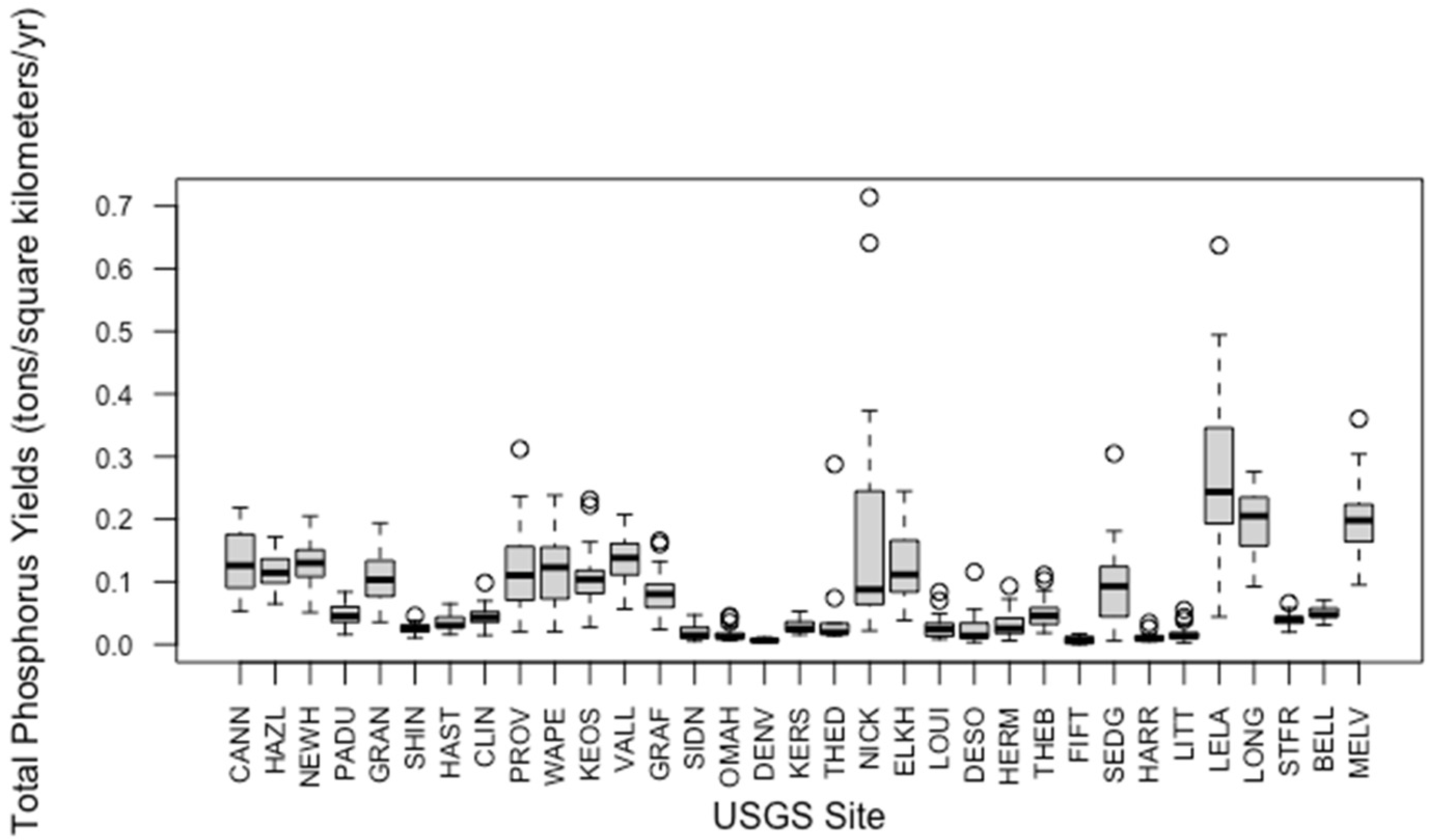
Figure 4.
Boxplot of the distribution of annual yields of silica.
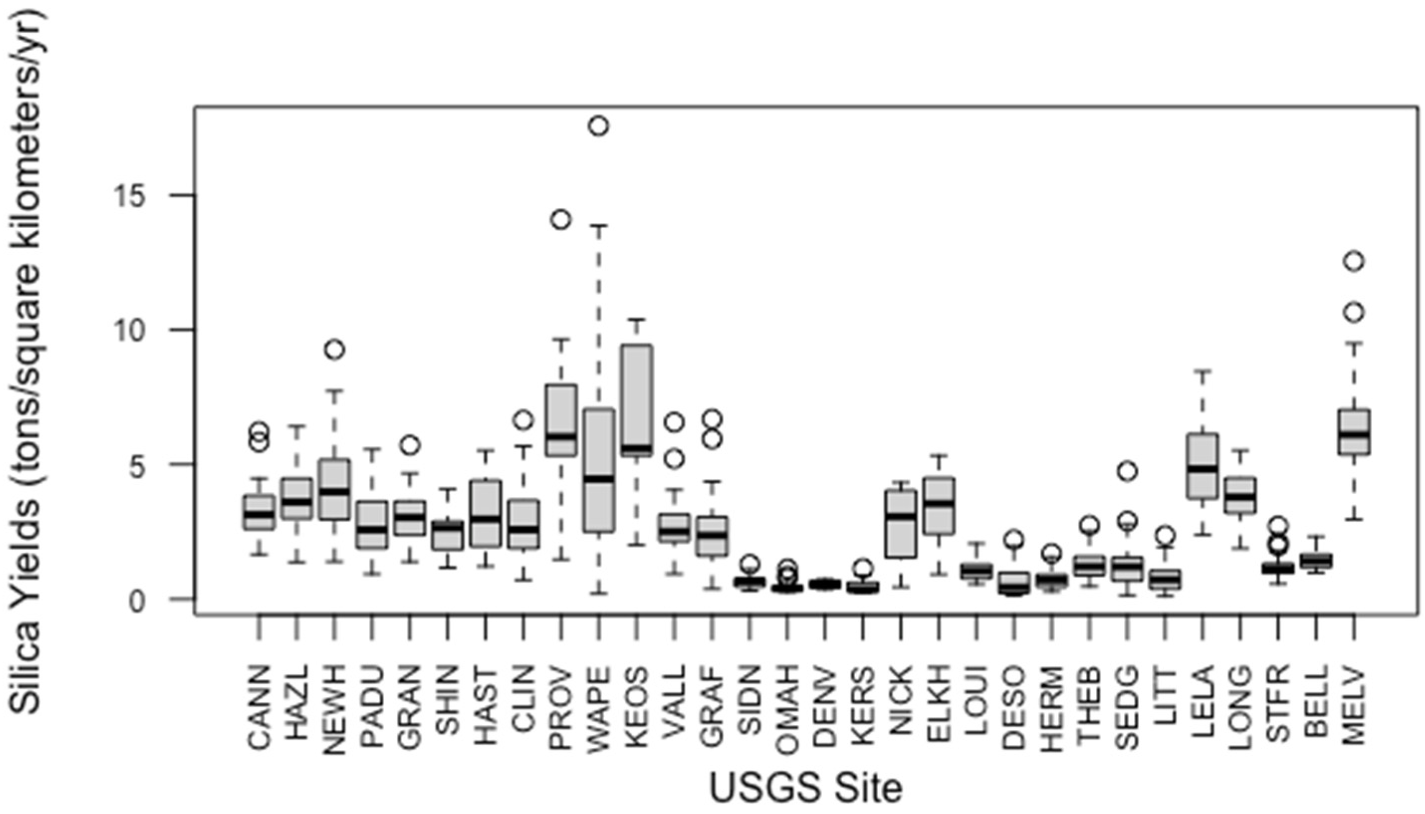
Figure 5.
Scree plot.
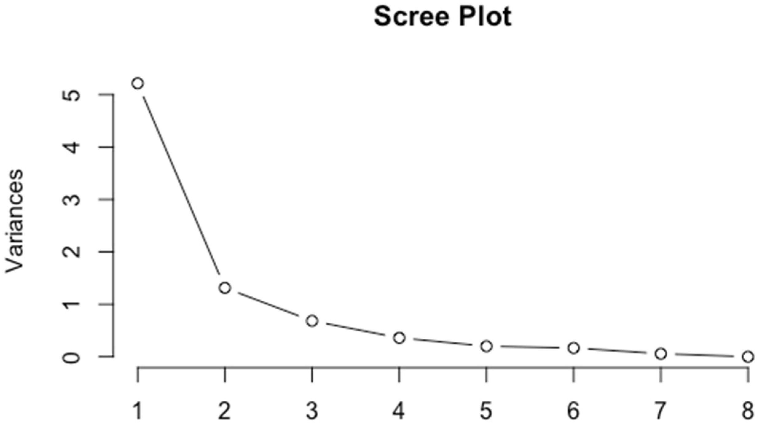
Figure 6.
PCA biplot.
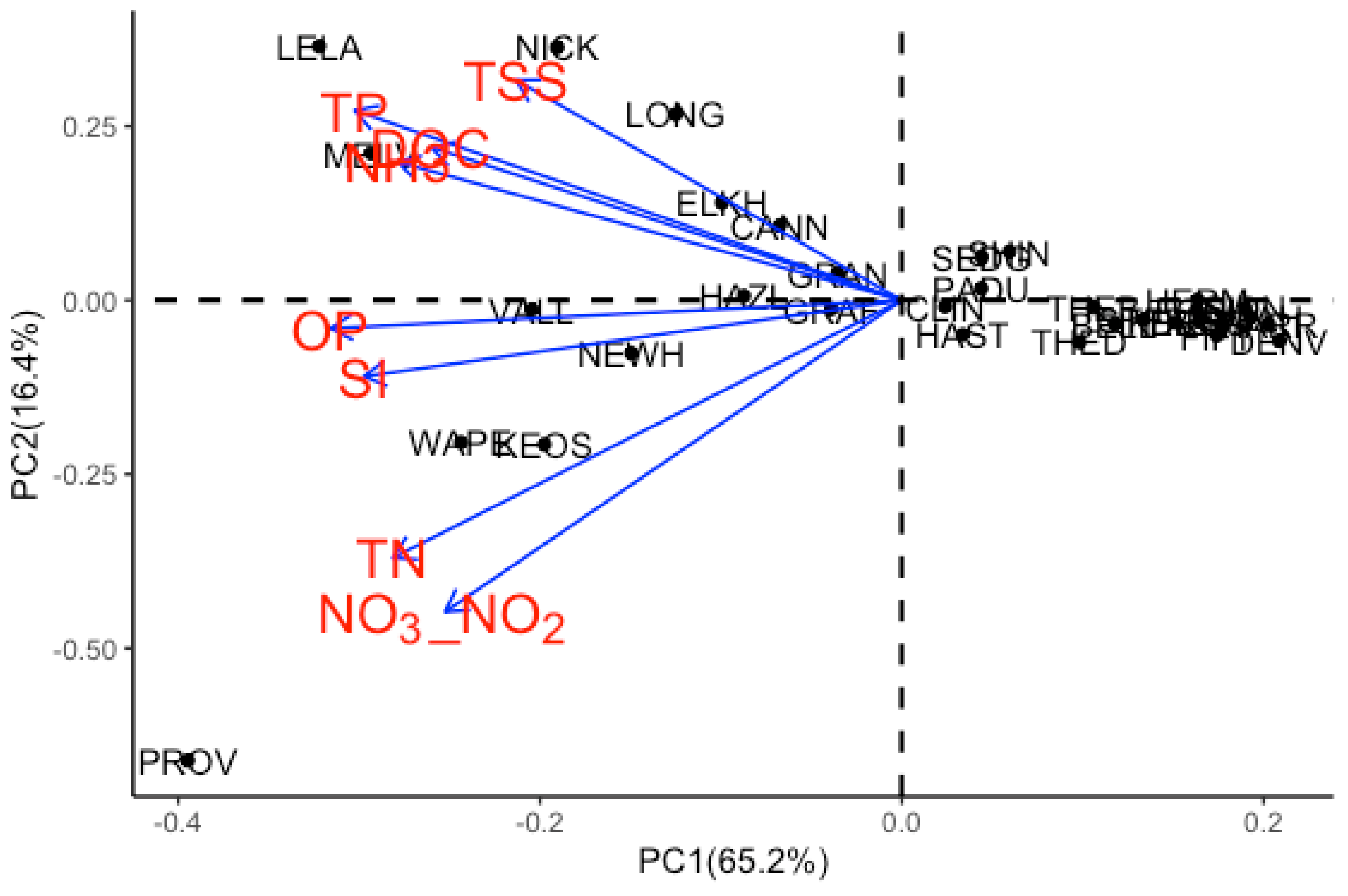
Figure 7.
Visualization of annual average nutrient yields from the 33 USGS monitoring stations produced using t-SNE.
Figure 7.
Visualization of annual average nutrient yields from the 33 USGS monitoring stations produced using t-SNE.
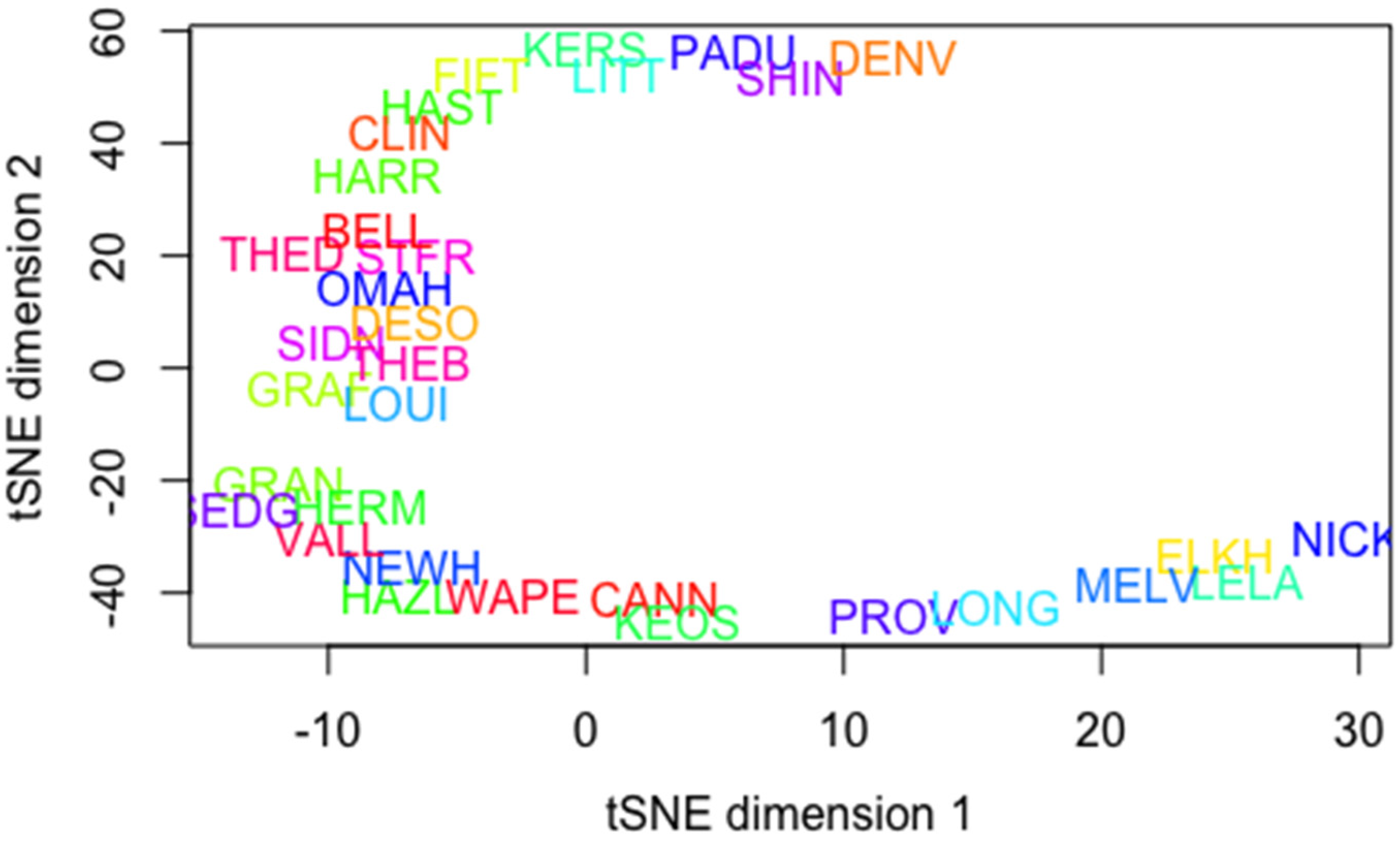
Figure 8.
Clustering annual average nutrient yields from the 33 USGS monitoring stations produced using K-means clustering analysis.
Figure 8.
Clustering annual average nutrient yields from the 33 USGS monitoring stations produced using K-means clustering analysis.
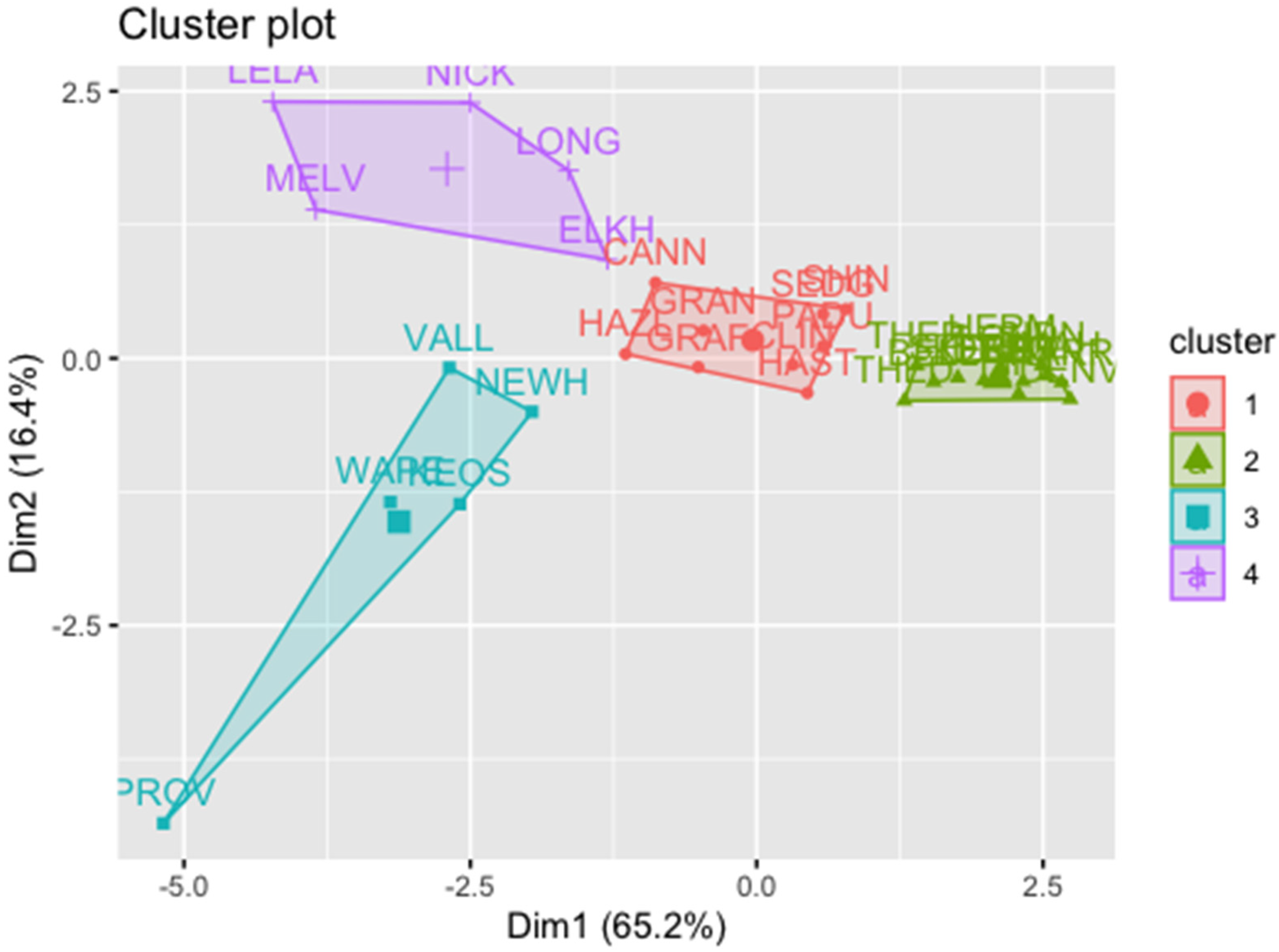
Figure 9.
Clustering annual average nutrient yields from the 33 USGS monitoring stations produced using hierarchical clustering analysis. Red, orange, and purple lines represent the heights of formations of two, three, and four clusters, respectively.
Figure 9.
Clustering annual average nutrient yields from the 33 USGS monitoring stations produced using hierarchical clustering analysis. Red, orange, and purple lines represent the heights of formations of two, three, and four clusters, respectively.

Table 1.
USGS water stations used in the study during 1996–2020 (https://www.sciencebase.gov/catalog/item/61c08ec5d34ee9cd54ed3425 (accessed on 22 May 2023).
Table 1.
USGS water stations used in the study during 1996–2020 (https://www.sciencebase.gov/catalog/item/61c08ec5d34ee9cd54ed3425 (accessed on 22 May 2023).
| SITE_ABB | SITE_QW_ID | Location |
|---|---|---|
| CANN | 3303280 | Ohio River at Cannelton Dam at Cannelton, IN |
| HAZL | 3374100 | White River at Hazleton, IN |
| NEWH | 3374100 | Wabash River at New Harmony, IN |
| PADU | 3609750 | Tennessee River at Highway 60 near Paducah, KY |
| GRAN | 3612500 | Ohio River at Dam 53 near Grand Chain, IL |
| SHIN | 5288705 | Shingle Creek at Queen Ave. in Minneapolis, MN |
| HAST | 5331580 | Mississippi River below L&D 2 at Hastings, MN |
| CLIN | 5420500 | Mississippi River at Clinton, IA |
| PROV | 5451210 | South Fork Iowa River NE of New Providence, IA |
| WAPE | 5465500 | Iowa River at Wapello, IA |
| KEOS | 5490500 | Des Moines River at Keosauqua, IA |
| VALL | 5586100 | Illinois River at Valley City, IL |
| GRAF | 5587455 | Mississippi River below Grafton, IL |
| SIDN | 6329500 | Yellowstone River near Sidney, MT |
| OMAH | 6610000 | Missouri River at Omaha, NE |
| DENV | 6713500 | Cherry Creek at Denver, CO |
| KERS | 6754000 | South Platte River near Kersey, CO |
| THED | 6775900 | Dismal River near Thed Ford, NE |
| NICK | 6800000 | Maple Creek near Nickerson, NE |
| ELKH | 6800500 | Elkhorn River at Waterloo, NE |
| LOUI | 6805500 | Platte River at Louisville, NE |
| DESO | 6892350 | Kansas R. at Desoto, KS |
| HERM | 6934500 | Missouri River at Hermann, MO |
| THEB | 7022000 | Mississippi River at Thebes, IL |
| FIFT | 7060710 | North Sycamore Creek near Fifty-Six, AR |
| SEDG | 7144100 | L. Arkansas R. NR Sedgwick, KS |
| HARR | 7241550 | North Canadian River near Harrah, OK |
| LITT | 7263620 | AR River David D. Terry L&D below Little Rock, AR |
| LELA | 7288650 | Bogue Phalia NR Leland, MS |
| LONG | 7288955 | Yazoo River BL Steele Bayou NR Long Lake, MS |
| STFR | 7373420 | Mississippi River NR St. Francisville, LA |
| BELL | 7374525 | Mississippi River at Belle Chasse, LA |
| MELV | 7381495 | Atchafalaya River at Melville, LA |
Note: SITE_ABB: a text abbreviation of the site name primarily for use within the National Water Quality Program; SITE_QW_ID: unique USGS station number indicating the location where water quality samples were collected.
Table 2.
Correlation coefficient matrix of eight parameters (note: bold typeface is used to show strong correlation coefficients).
Table 2.
Correlation coefficient matrix of eight parameters (note: bold typeface is used to show strong correlation coefficients).
| DOC | NH3 | NO3_NO2 | OP | SI | TSS | TN | TP | |
|---|---|---|---|---|---|---|---|---|
| DOC | 1.00 | |||||||
| NH3 | 0.68 | 1.00 | ||||||
| NO3_NO2 | 0.31 | 0.42 | 1.00 | |||||
| OP | 0.62 | 0.72 | 0.70 | 1.00 | ||||
| SI | 0.68 | 0.57 | 0.69 | 0.77 | 1.00 | |||
| TSS | 0.35 | 0.55 | 0.23 | 0.52 | 0.40 | 1.00 | ||
| TN | 0.42 | 0.52 | 0.99 | 0.76 | 0.74 | 0.33 | 1.00 | |
| TP | 0.79 | 0.77 | 0.39 | 0.80 | 0.70 | 0.73 | 0.51 | 1.00 |
Table 3.
Loadings of eight variables in two principal components.
| Eigenvalues | 5.22 | 1.31 |
|---|---|---|
| Cumulative (%) | 65.2 | 16.4 |
| Principal Component(PC) | PC1 | PC2 |
| DOC | −0.33 | 0.28 |
| NH3 | −0.36 | 0.25 |
| NO3-NO2 | −0.32 | −0.57 |
| OP | −0.40 | −0.05 |
| SI | −0.37 | −0.14 |
| TSS | −0.27 | 0.40 |
| TN | −0.36 | −0.47 |
| TP | −0.39 | 0.35 |
Table 4.
Principal component scores.
| USGS Monitoring Site | PC1 | PC2 |
|---|---|---|
| CANN | −0.88 | 0.71 |
| HAZL | −1.15 | 0.04 |
| NEWH | −1.96 | −0.50 |
| PADU | 0.57 | 0.11 |
| GRAN | −0.46 | 0.26 |
| SHIN | 0.78 | 0.46 |
| HAST | 0.44 | −0.32 |
| CLIN | 0.31 | −0.06 |
| PROV | −5.18 | −4.35 |
| WAPE | −3.19 | −1.34 |
| KEOS | −2.59 | −1.36 |
| VALL | −2.68 | −0.08 |
| GRAF | −0.51 | −0.08 |
| SIDN | 2.49 | −0.06 |
| OMAH | 2.53 | −0.16 |
| DENV | 2.74 | −0.38 |
| KERS | 1.98 | −0.20 |
| THED | 1.28 | −0.40 |
| NICK | −2.50 | 2.39 |
| ELKH | −1.30 | 0.92 |
| LOUI | 2.14 | −0.09 |
| DESO | 2.16 | −0.20 |
| HERM | 2.15 | 0.003 |
| THEB | 1.39 | −0.07 |
| FIFT | 2.29 | −0.33 |
| SEDG | 0.58 | 0.41 |
| HARR | 2.66 | −0.22 |
| LITT | 2.32 | −0.22 |
| LELA | −4.23 | 2.40 |
| LONG | −1.64 | 1.76 |
| STFR | 1.76 | −0.18 |
| BELL | 1.55 | −0.22 |
| MELV | −3.85 | 1.39 |
Disclaimer/Publisher’s Note: The statements, opinions and data contained in all publications are solely those of the individual author(s) and contributor(s) and not of MDPI and/or the editor(s). MDPI and/or the editor(s) disclaim responsibility for any injury to people or property resulting from any ideas, methods, instructions or products referred to in the content. |
© 2023 by the authors. Licensee MDPI, Basel, Switzerland. This article is an open access article distributed under the terms and conditions of the Creative Commons Attribution (CC BY) license (https://creativecommons.org/licenses/by/4.0/).
Share and Cite
MDPI and ACS Style
Zhen, Y.; Feng, H.; Yoo, S. Structuring Nutrient Yields throughout Mississippi/Atchafalaya River Basin Using Machine Learning Approaches. Environments 2023, 10, 162. https://doi.org/10.3390/environments10090162
AMA Style
Zhen Y, Feng H, Yoo S. Structuring Nutrient Yields throughout Mississippi/Atchafalaya River Basin Using Machine Learning Approaches. Environments. 2023; 10(9):162. https://doi.org/10.3390/environments10090162
Chicago/Turabian StyleZhen, Yi, Huan Feng, and Shinjae Yoo. 2023. "Structuring Nutrient Yields throughout Mississippi/Atchafalaya River Basin Using Machine Learning Approaches" Environments 10, no. 9: 162. https://doi.org/10.3390/environments10090162
Note that from the first issue of 2016, this journal uses article numbers instead of page numbers. See further details here.