Spectral Index-Based Monitoring (2000–2017) in Lowland Forests to Evaluate the Effects of Climate Change


1
Department of Physical Geography and Geoinformatics, University of Szeged, Egyetem str. 2-6, 6722 Szeged, Hungary
2
Department of Physical Geography and Geoinformatics, Doctoral School of Earth Sciences, University of Szeged, Egyetem str. 2-6, 6722 Szeged, Hungary
*
Author to whom correspondence should be addressed.
Geosciences 2019, 9(10), 411; https://doi.org/10.3390/geosciences9100411
Submission received: 16 August 2019
/
Revised: 11 September 2019
/
Accepted: 19 September 2019
/
Published: 23 September 2019
(This article belongs to the Special Issue Remote Sensing used in Environmental Hydrology)
Abstract
:In the next decades, climate change will put forests in the Hungarian Great Plain in the Carpathian Basin to the test, e.g., changing seasonal patterns, more intense storms, longer dry periods, and pests are expected to occur. To aid in the decision-making process for the conservation of ecosystems depending on forestry, how woods could adapt to changing meso- and microclimatic conditions in the near future needs to be defined. In addition to trendlike warming processes, calculations show an increase in climate extremes, which need to be monitored in accordance with spatial planning, at least for medium-scale mappings. We can use the MODIS sensor dataset if up-to-date terrestrial conditions and multi-decadal geographical processes are of interest. For geographic evaluations of changes, we used vegetation spectral indices; Enhanced Vegetation Index (EVI) and Normalized Difference Vegetation Index (NDVI), based on the summer half year, 16-day MODIS data composites between 2000 and 2017 in an intensively forested study area in the Hungarian Great Plain. We delineated forest areas on the Danube–Tisza Interfluve using Corine Land Cover maps (2000, 2006, and 2012). Mid-year changes over the nearly two-decade-long period are currently in balance; however, based on their reactions, forests are highly sensitive to abrupt changes caused by extreme climatic events. The higher occurrence of years or periods with extreme water shortages marks an observable decrease in biomass production, even in shorter index time series, such as that between 2004 and 2012. In the drought-stricken July-August periods, the effect of a dry year, subsequent to years with more precipitation, immediately pushes back the green mass and the reduction in the biomass production could become persistent, according to climatology predictions. The changes of specific sub-periods in the vegetation period can be evaluated even in a relatively short, 18-year data series, including the change in the growing values of the vegetative growth in spring or the increase in the summertime biomass production. Standardized differences highlight spatial differences in the biomass production; in response to years with the highest (negative) biomass difference; typically, the northern and southwestern parts of the Danube–Tisza Interfluve in the study area have longer lasting losses in biomass production. A comparison of NDVI and EVI values with the PaDI drought index and the vegetation indices of LANDSAT Operational Land Imager sensor respectively confirms our results.
1. Introduction
The magnitude of the geographical consequences of processes characterized by climate and land use changes plays a substantial role in the quest for higher temporal and geometrical resolutions in environmental monitoring systems [1,2]. Continuous and up-to-daily temporal resolution data acquisitions, which started in the 1970s with the NOAA AVHRR satellite observations and were followed by the LANDSAT, SPOT and MODIS programs, enable us to study recent and multi-decadal environmental processes based on multi-resolution databases of various satellite sensors. We can analyze the changes in enviro-climatic processes as well as their effects on shorter and longer time periods.
The key question addressed by regional or local scale environmental studies is how agriculture and forestry will cope with the continuously evolving climatic conditions in the near future, that is, in the next decade. According to the current Paris Climate Agreement, a global temperature increase of over +2 °C is expected to occur by 2100, which would amplify global economic effects currently leading to decreases of 23% in the gross domestic product [3]; Central Europe, and therefore Hungary, belongs to one of the regions exhibiting higher warming rates than the global mean.
Climate change induced processes, such as aridification, lead to higher complexity problems due to the interconnected nature of landscape factors. Today, irreversible changes in some areas cannot be mitigated, even with extreme water amounts [4]. In addition to landscape factors, ecosystem services add character to the landscape, highlighting the importance of vegetation as a landscape factor. Based on the number of species, 58% of the global land surface is biologically compromized (71.4% of the human population lives in these areas) and ongoing human intervention may be needed to ensure the delivery of ecosystem functions [5]. Biospheric changes (e.g., albedo changes) feedback on climatic change; therefore, it is important to have accurate and up-to-date information on the state of the vegetation. Therefore, it is not a coincidence that continental-scale vegetation and vegetation change datasets are also currently being produced at resolutions of 20 m [6]. Vegetation as a climate indicator is also an indicator of short-term changes, extremes, and trend-like changes that can be measured and assessed everywhere with a fully developed remote sensing methodology.
In creating local and regional land uses fitted to climatic conditions, the main goal is the conservation of ecosystems depending on forestry. Forests are the only land ecosystems that extract CO2 from the air and therefore slow the increase in its atmospheric concentration, thereby moderating the rate of climate change. The Hungarian forests alone are extracting more than 3 million tons of CO2 from the atmosphere annually. These phenological estimates, which are concerned with the relation between the carbon- and water cycles and the forests, and their relation to climate change, are critically important.
Based on the drought-sensitivity and vulnerability of forest ecosystems, Hungary is one of the regions worldwide that are highly endangered by climate change [7]. We need to adopt decades-long forestry strategies that require a new mindset due to the climate change. According to the National Landscape Strategy (2012–2020) [8], to achieve the 26% forest coverage goal, 600,000–750,000 ha of afforestation is required over the next 35 years. In the meantime, climate change may challenge forests, e.g., via changing seasonal patterns, more intense storms, longer dry periods, and pests are expected to happen. To aid in the decision-making process, it should be defined how forestry could adapt to changing mezo- and microclimatic conditions in the near future needs to be defined.
To understand the landscape degradation problems caused by climate change, it is necessary to observe the vegetation, particularly the forest-covered areas on a local/regional scale. The Danube–Tisza Interluve contains extensive forest-covered areas, despite the fact that it is a lowland region, and is one of the regions with the most intense afforestation activity in Hungary. One question is whether the process of climate change is recognizable on various temporal scales for woody vegetation, e.g., on its growth and phenological phases. How much of a difference in productivity would be caused by more frequent extreme water balance situations? The adaptation capacity via deviations from the average can express how the vegetation factor is capable of fending off the negative effects of gradual (e.g., aridification) and abrupt changes (e.g., drought). Remote sensing monitoring can be used to quantify these effects. Studies have verified moderate-resolution satellite products with in-situ point measurements (and the empirical indices based on them); therefore, we can provide information on large areas and at better spatial resolution for regional forestry planning. This would provide good results toward the final goal, realizing automatized change detection, because such changes are not temporary or isolated events; accordingly, there is a need for a regional development strategy.
1.1. The Study Area and the Delineation of Forests
Vegetation change is an applied indicator that connects climate change to the landscape [9], and monitoring provides a tool to determine the value of this change. In the Carpathian Basin, more specifically on the Hungarian Plain, on the Danube–Tisza Interfluve, in areas stricken by weather extremes, not only the climatic conditions, but also the land cover is heterogeneous. The summer-half-year monitoring of forests between 2000 and 2017 was performed between days 81 and 288 of each year. We examined data cells in raster graphics of 250 m-resolution MODIS satellite images (see the data description in Section 2.1); two-thirds of which are covered with deciduous, or with coniferous, or with mixed forests based on the Corine Land Cover (CLC) datasets of 2000, 2006 and 2012 [10], where each forest patch is made up of at least three raster cells. The other pixels were subtracted from the evaluation. Therefore, the forest cells as determined by satellite images cover 71–85% of all the forests in the region (Figure 1). Deforestation and the forestry management works in the region might affect the results; however, based on the CLC layers, deforestation only affected 1.5% of forests between 2000 and 2006 and, at maximum, 7–9% of forests between 2006 and 2012. A test analysis of deciduous forests with constant coverage (with no deforestation throughout the years) confirmed that these spatial alterations have a negligible effect on the results. The forest coverage was 132,296 ha in 2012.
Seasonal, continuous mid-year, and sudden changes can be differentiated using homogeneous cells at the applied geometric resolution [12]. Aridification is causing ecologic transformation at the landscape level, for which low-resolution data are suited. Conversely, human-caused changes are taking place on time scales of days and at smaller spatial scales [13]. Reference [14] classified cells with more than 20% coverage as “agricultural” and Reference [13] used 60% coverage in the case of forests, whereas Reference [15] used 75% coverage. Reference [16] used a more homogenous delineation because they used cells with 90% coverage that were unchanged according to the MCD12Q1 500 m data product however with these conditions, only a quarter of the original area can be analyzed.
1.2. The Environmental Problem in the Study Area: Consequences of Climate Change for the Landscape
Global warming is more easily verifiable. According to NASA, by the summer of 2016, the global monthly warm temperature records were broken in seven consecutive months and July 2016 was the hottest month in the 137-year temperature records [17]. The year 2018 was one of the warmest years in weather history despite the fact that no (natural) anomaly (such as El Nino) could account for it. In the period of 931−2005, based on tree ring data, the six hottest years were between 2000 and 2005 [18]. In a climatically relatively homogenous environment such as Hungary, it is not easy to detect regional differences [19]. In the last decades, extremes have dominated, and inland excess water and aridification can occur at the same time [20]. Multiple times in recent years, the annual precipitation amount differed by at least 200 mm from the previous year [21]. Based on measurements, in Hungary, 2010 was the wettest and 2011 was the driest years ever. The dual nature of the annual precipitation amount is characterized by the fact that, in addition to the wettest years of 1998, 1999, 2005, and 2010, the years 2000, 2013, and 2011 were among the seven driest years on record.
In our study area in the last 30 years, the mean temperature increased by 1.2–1.5 °C, the summer days increased by 20–30 days, and the biggest temperature increase was +2.2° C in the summer, with areas above a mean temperature of 11 °C appearing [22,23] (Figure 2). According to climate models, the growing period, which is characterized by Tmean > 5 °C, might increase by 24 days compared to the 1960–1990 reference period. The annual mean warming is in these models is between 1.1 °C and 1.7 °C, whereas the summer mean warming is between 1.4 °C and 3.7 °C [24,25].
The incidence rate of the months above the average temperature and below the average precipitation was 40% during the period of 2000–2017, and these differences were characteristic primarily in the spring. Between 1995 and 2017, only 8 years can be considered to be drought-free (Figure 3). In 14 years, the spatial ratio of drought-stricken areas was greater than 70% seven times. The average of the annual Pálfai Drought Index (PaDI) generally known in the Carpathian Basin, calculated using the temperature, precipitation, and groundwater level increased from 4.4–5.5 (during the period of 1961–1987) to 5.6–6.6 (during the period of 1988–2012) [27]. The soil being a natural water storage medium can moderate precipitation extremes; however, only 19% of the soils in the study area are considered as having good water storage capacities.
Owing to trend-like changes, the Danube–Tisze Interfluve has a 9 km3 groundwater deficit and this change is irreversible in 1500 km2 of the region. A wet year can cause approximately 2 km3 change in the water supply; however, one or two wet years only enables partial water refilling at the mesoscale [4]. Based on a 130-year time series, in response to more precipitation, lakes, swamps, and marches are being partially regenerated for shorter time periods; however, a quarter of these areas are drying up [28].
1.3. Environmental Problems in the Study Area: Climate Change and Forests
A total of 80% of tree growth can be realized with intensive water usage between May and July. Therefore, the springtime precipitation decreases and the 4–5 subsequent dry summers typical in the last decades are crucially important [7]. The dryness of the Danube–Tisza Interfluve is amplified by the fact that 98% of the underlying soils in these forests have a weak water storage capacity.
The state of the woody vegetation is an integral, and its productivity is influenced by past effects and therefore the annual average does not necessarily accurately reflect its quality; regarding climate change, we cannot draw any conclusions solely from current observations [16]. The forests store carbohydrates, which, for a given time, compensate for the nutrient deficit and the lack of photosynthetic carbon; however, the regenerative capacity of lowland forests is generally small.
Tree flowering in Hungary currently starts 3–8 days earlier than it did 100 years ago. By the 1990s, the flowering of black locust trees (Robinia pseudoacacia), which makes up 20% of all domestic forests, was only sustained until the end of May [30]. From 1952 to 2000, the flowering time of black locust changed by 1.9–4.4 days per decade, which was confirmed by measurements in the period of 1984–1997 [31].
A total of 80% of forests are not native to the Danube–Tisza Interfluve, and these forests primarily exist for timber production (76%). The landscape, natural capital index based on habitat volume and quality [32] is on average 7.7% (max. 32%) for coniferous forests, 5.8% (max. 28%) for deciduous forests, and 7.1% (max. 32%) for mixed forests. The foliage of 75% of the forests is closed by a minimal coverage of 50% (see Figure 1).
Forests primarily exert their effects locally on the underground water level and on its decreases locally. According to Reference [33], forestation with land use change accounts for 10% of the water level decrease, whereas according to Reference [34], the increase in forest area is only responsible for 13–15% of the decrease.
2. Materials and Methods
2.1. Multispectral Data Products
The main remote sensing data for regional scale observations are MODIS data. Phenological processes require the combined usage of Terra and Aqua carriers; however, the correlation coefficients of these sensors are very weak; accordingly, for an analysis, only one is used in general and the surface reflectance correlation is better in the case of Terra [35]. The MODIS Maximum Value Composite (MVC) data product assigns the highest Normalized Difference Vegetation Index (NDVI) value to each cell in 16-day periods, where the value is determined by the image cell with the lowest viewing angle from the 5–10 images retained after the quality assessment. A total of 87% of the pixels in the composites are in the ±30° viewing angle range [36]. Due to the image processing, the composite image is closer to the field data than the daily reflectance data because the pixel size, the viewing angle of the sensor, and the covered area are variable from day to day. As a result, the variability in the reflectance could originate from the variable spatial coverage, and not from the actual changes [13,37].
In our study, we used versions 5 and 6 of the 16-day, daily reflectance-based, 250 m spatial resolution MOD13Q1 composite product. A detailed analysis of the quality assurance data was conducted by using programming solutions (i.e., scripts) [38]. We only analyzed dates when at least 80% of the forest cells had good quality; therefore, we were able evaluate 97% of the entire 18-year study period.
For the validation of small-scale satellite images, we used multispectral images with better resolution captured by the LANDSAT OLI (Operational Land Imager) instrument as a “virtual field observations” [39,40,41]. In this case, the spectral indices also used for MODIS satellite were derived from the Level-2 and 30-m-resolution images [42]. We looked for a period when the most cloud-free imagery was available within a year, and we found eight OLI images with good quality to the southern part of the sample area in the spring and in the summer of 2015; 16. April, 18. May, 03. June, 05. July, 21. July, 06. August, 07. September, and 23. September.
2.2. The Usage and Application of Spectral Indices
A total of 90% of vegetation information has been measurable with spectral indices since the 1970s [43]. The goal of such indices is to enhance the vegetative response and to reduce the soil brightness and color, atmospheric effects, shadows, and moisture content. These indices correlate with the field leaf area index (LAI) and fraction of absorbed photosynthetically active radiation (fAPAR) measurements [14]. The 16-day MVC vegetation index (VI) data, with angle- and atmospheric-dependences, gives good estimates matching those of aerial surveys [40].
Vegetation index datasets are good phenological indicators; however, this multispectral landscape phenology is different than the phenology characterized by individual-level morphologic properties [30]. At an appropriate scale, despite interfering factors, vegetation indices with normalization describe the vegetation well within empirical value ranges. Drought levels can be characterized by the vegetative characteristic contributing to the decrease in their effects [44].
NDVI and EVI as Vegetation Indices
For our vegetation monitoring, we chose the MOD13Q1 NDVI and Enhanced Vegetation Index (EVI) datasets between 2000 and 2017, and analyzed 457 satellite images:
where NIR indicates the near infrared band, Red indicates the visible red band, Blue indicates visible blue band, L = 1, C1= 6, C2 = 7.5, and G = 2.5.
Due the errors in the atmospheric correction, i.e., errors originating from the uncertainty of the calibration, the Rayleigh scattering error, and ozone absorption [45] an acceptable MODIS NDVI error of +/–0.04 can be calculated, which could be significant in time series exhibiting only small change values. This index may be overestimated at the start of the summer half year and underestimated at the end of the summer half year. The greening is due to the parts under the canopy, which can reach 14% of the examined quantity. This could be the cause of earlier greening and the stable VI maximum at the defoliation time. NDVI values of high-biomass forests have a tendency to saturate but are appropriate for surface change assessment in biologically complex areas [14,46]. Owing to its sensitivity to the surface heterogeneity, the vegetation cover needs to be delineated. In the case of seasonal analyzes with small seasonal variations, drought is not always prominent.
In global observations, AVHRR NDVI was replaced by MODIS EVI solutions [45]. EVI is more stable due to the usage of the visible blue band. It has sensitivity to high biomasses; the difference in the EVI values between coniferous and deciduous forests is 1.5-fold. A deciduous forest is detected if EVI exceeds 50% of the maximum in an annually time series [41]. At the time of defoliation, the decrease is more significant [40]. EVI has a smoother, more symmetric seasonal profile with a better-defined peak; its value is lower than that of NDVI, and this narrower value range is an advantage in the elimination of “saturation.”
NDVI and EVI complement each other; therefore, so change detection and the extraction of biophysical parameters can be performed more successfully. For example, in the 32-day MODIS MVC dataset, NDVI was more accurate when studying forests and shrubs [47]. Usually, the index values in the case of forests do not correlate well. However, the results in our study area do not support this; the deciduous and mixed forests had a strong correlation calculated by Pearson’s method (rdeciduous = 0.95123; rmixed = 0.8582). The saturation problem is characterized by the difference in the index values, which is higher for grasslands/shrubs (EVImax = 0.4 and NDVImax = 0.7) than for forests (EVImax = 0.8 and NDVImax = 0.9) [40]. Based on regional and national averages and the differences calculated for vegetation surfaces, we cannot state that one index is better than the other one in every aspect [16,44,48].
The variability of the standardized anomalies is informative during monitoring.
where i and j indicate the row and column numbers of the current cell, Zi,j indicates the standardized vegetation index, Xi,j indicates the current value of the index, indicates the average of index values for the reference period from 2000 to 2017, and SDi,j indicates the standard deviation of the spectral index values for the reference period.
The forestry forest-state monitoring system also uses the MODIS-based standardized NDVI/EVI anomalies. For the different land cover types, drought years (e.g., 2012) are defined by the standardized negative anomalies of these indices [16,49]. In assessments, it is very important that, while cropland and meadows/pasture indicators are consistent, forests have different behaviors and do not necessarily have similarities to meteorological anomalies. Based on data series from Central-European countries between 2000 and 2014, there is not a single year having a general effect that applies to all forests [16].
In the phenology for the time period between DOYs (day-of-year) 120 and 200 evaluated using the MODIS products, the best match was found between the starting time of the canopy closure and the 1 km MOD15 LAI data, which only differed by 7% from the maximum of the field measurements. According to daily MOD09 NDVI, there is a 21-day gap between the greening and the start of canopy closure; therefore the 16-day MVC under-, or over-estimates the phenological state. Accordingly, we could increase the temporal resolution to just under seven-week value [45]. The connection between the field and MODIS NDVI measurements in the case of deciduous forests is significant mainly during the greening and vegetation densification periods [37]. The inflection points of the fitted model match the greening (spring) and yellowing (autumn) time with less than one-week difference. The 16-day MODIS maximum is suitable to create the springtime NDVI curve and, based on that, to determine the inflection point with 1.5–7 days of difference, because its pre-processing is more reliable than that of the daily data.
In the case of regional-scale assessments focusing on forest land usage, productivity does not necessary develop in accordance with climate-change fluctuations because, at a larger scale, climate is not necessary the dominant factor in the development of vegetation. Based on the forest-covered areas in the Danube–Tisza Interfluve, climatic effects can be evaluated with at least a decade of biomass production data [50].
2.3. PaDI as the Index of the Validation
By studying various surface cover types in Hungary, the strongest link was found between NDVI and temperature [14]. In our study area, dry periods and dense vegetation also occur; therefore, we looked for connections with the PaDI index [27].
where TApr-Aug indicates the mean monthly temperature from April to August, POct-Aug indicates the monthly sum of precipitation from October to August, wi indicates the weighting factor expressing the importance of the months in the evolution of drought, kt, kp, and kgw are the correction factors assessing the temperature, precipitation, and groundwater conditions in the preceding years.
The 10-km resolution PaDI model values calculated on the basis of field stations are available for the period of 2000–2010 in the CARPATCLIM database [51].
3. Results and Discussion
3.1. Evaluation of Forest Vegetation with EVI/NDVI between 2000 and 2017
High index values in the 2000–2017 data series prove the accuracy of the forest delineation and the legitimacy of taking both indices into account on the basis of their differences in the examined 18-year period. The median values show the NDVI saturation problem: 0.37 < NDVIdeciduous < 0.85 and 0.17 < EVIdeciduous < 0.59. As a result, EVI is more responsive to changes in biomass production and reacts more regularly and more sensitively to external influences, making dry periods conspicuous (Figure 4). The average year in the data series was 2013, which is only specific to EVIdeciduous and EVImixed. Owing to the 25% median value differences between deciduous and coniferous forests, different types of vegetations are more distinguishable using EVI. The relative runs of the curves of different forest categories are similar; therefore, missing values can be given according to the data of the other forest types and a complete data series can be considered. For the deciduous EVI, we created a test series limited to permanent forest areas as defined by CLC 2000–2012, which confirmed that the applied forest area differences between CLC2000, CLC2006, and CLC2012 do not affect the values for the entire study area over the 18 years.
Despite the aridification impacting the study area, the NDVI and EVI medians, sums and extreme values of the entire time series between 2000 and 2017 do not exhibit a significant trend-like change, in which the higher VI values in the 2014–2017 period played the main role due to the more favorable environmental conditions. The most intensive mid-year change is the springtime growth of the deciduous forests when the vegetation quantity can increase by 35–65% within a single month.
The median VI values and the sum obtained by adding the cell values decreased more rapidly in years with less precipitation and those generally exhibiting warming; this is seen between 2006 and 2007. Higher values in single wet years (such as 2010) and lower values in single drought years (2015) are not extraordinary due to the effects of the surrounding years. By comparing the periods of 2003–2004 and 2012–2013 years, it is clear that the low value of a drought year in the case of water resupply rapidly increases; this translates to an 8–10% increase in the deciduous biomass production. The order of years with the smallest VI values is 2012, 2003, and 2009, whereas that of the years with the highest values is 2016, 2017, and 2008. The year 2008, was one of the most productive years despite the fact that it was not backed up by meteorological conditions. After 2012, the effect of the drought years 2013, 2015, and 2017 did not show up in the statistical values. From 2013 to the present, biomass production has generally been increasing, whereas the drought-stricken area often has a value of 80–89% according to national data (see Figure 3). A given month in a wetter year can have EVI values as low as the same period in a drier year; the wet year of 2010 had the lowest end of the May–June EVIdeciduous value; conversely, the drought years of 2003 and 2012 had above-average values in June.
The sum of biomass production for the period of 2004–2012 has a decreasing trend; however, if we only take into account the more recent 2009–2017 period, we see growth. Dry periods with a maximum of 5 years are usually intercepted by a year with more precipitation, which is sufficient for the woody biomass production to not decrease regionally in the longer term [49]. Years marked by biomass production periods of 4–5 years are not necessarily the same for different types of forests. The shorter 2001–2003, the characteristic 2006–2009 (in the case of NDVIdeciduous: 2005–2009), and the 2010–2014 (in the case of NDVI: 2010–2013) periods experienced a decrease in the EVI/NDVI median values. They fit well into periods of warmer and drier weather and low groundwater levels [28]. The 2014–2017 period had a growing, stable biomass production in the last 18 years, even though there were also several drought years in that period. Over 18 years, the total value of the deciduous biomass increased.
The value of VIdeciduous shows a trend-like growth in the spring period from March 22–May 8 (Figure 5). Between the periods of 2000–2006, 2007–2013, and 2014–2017 the value of VI increased by a total of 14–25%, which indicates a more intensive greening due to warming [31]. At the same time, the rising EVImixed values of the last September 30–October 15 period together with rising springtime values support growth during the entire vegetation period. The fact that greening comes earlier, while leaf fall shifts toward later dates, is in agreement with phenological observations in Europe [53]. In contrast to the increasing values of vegetation growth in the spring, the time to reach the biomass production peak (May 25–July 11) and the amount of deciduous productivity did not change. In the case of the EVIconiferous and EVImixed values, the summer peak of the biomass production shifted; this was mainly achieved by vegetation in early June between 2000 and 2007, which has shifted to the late-June and July periods [50]. During the June 10–July 11 period, growth can be detected during the 18-year period. In these types of forests, secondary peak values are frequent, which, in addition to increasing production values, suggests stable vegetation and therefore our values do not support predictions made about the weakening of pine forests.
It is beneficial that, in our analysis, there is no visible link between monthly intense water use and a significant reduction in the springtime precipitation (according to climatology) in the March–May–July period when 80% of tree stock growth occurs. In the spring period (April 23–May 8) in the case of NDVIdeciduous longer critical periods showing decline were observed between 2000 and 2006 and during the peak period (June 26–July 11) between 2006 and 2012. A geographical relation can be seen in 2001, 2004–2006, 2008, 2010, 2014, and 2016, when the precipitation exceeds the multi-year average and the temperature in the summer semesters is around the average or cooler, therefore leading to richer vegetation and two-peak VI curves. When examining MODIS biomass production, the precipitation in the March–May period and in June was the determining factor [20].
In the main drought period between July 12–September 13, the year-to-year fluctuations increase. In response to a dry year, the green mass instantly decreases, in other words, the woody vegetation is a fast indicator of environmental change [54]: primarily between 2000/2001 and 2006/2007 and in the summer periods between 2003/2004 and 2010/2011–2012. Starting in 2007, the period of July 28–August 28 has become critical because there are more below-average values during this period.
3.2. Analysis of Standardized Deviations from the EVI Mean
Owing to the sensitivity observed in the MODIS index data series, the standardized deviation was only evaluated for EVI in this study. In the standardized EVI deviation time series, the years showing negative anomalies are the same for every forest type and the drought years can be easily identified (Figure 6). This is clear in 2003, which had the greatest drought, whereas similar negative anomalies were observed in deciduous forests in 2012 and in coniferous forests in 2009. The worst period is the 2007–2012 6-year period, which had four below-average years. In the 2004–2006 period, which had positive EVI anomalies in general, deciduous forests continuously declined, whereas coniferous forests expanded. Between 2013 and 2015, the deciduous forest anomaly was larger and, until 2017, the biomass product surplus was constant in deciduous and coniferous forests.
Pixel-based, temporal and spatial analyzes through forest areas can indirectly indicate surfaces threatened by reductions in biomass quantity (Figure 7). Lasting deviations indicate vegetative responses to the effects of water shortages due to climate change. Seven below-average years exist between 2000 and 2017, i.e., the degree of positive anomalies could be higher but are slight for mixed forests and cannot be spatially generalized.
The years 2004, 2008, and 2016 can be considered to be the years with the most abundant vegetation based on the standardized EVI deviation maps. Of the drought years, the years 2003, 2009, and 2012 significantly affected the entire study area. In these years, there are 35–40% more negative anomalies than in the drought years of 2000, 2002, 2007, and 2011. The negative period of 2007–2012 with below-average values in the southern and northern parts of the Danube–Tisza Interfluve, based on spatiality, can be extended to the period between 2006 and 2014/2015; therefore the regionally increasing VI values characterized from 2013 do not apply to every area based on the spatial distribution. In the southern part of the study area, negative anomalies are specific even in the favorable year of 2000 and drought conditions are constant between 2009 and 2012. In the generally average and positive-anomaly years of 2014 and 2015, multiple negative values concentrating at specific locations can be observed. In contrast to the production increase from 2013 (significant growth percentages exceeded 35–40%), the decline in the period of 2014-2015 was greater than 40%.
The highest precipitation year of 2010 showed significant spatial deviations due to rainfall patterns and environmental effects; therefore, the study area can be split into two parts. The southern part has many negative anomalies even in 2010 (that is why it did not show increased biomass production in the statistics). Compared to the fact that 2010 was not a drought year in the time series, according to the EVI anomaly maps, more than 30% of forests have negative anomalies. This highest precipitation year is followed by 2011, which had the driest conditions and, in turn, resulted in significantly decreases in the green mass growth, increasing negative deciduous deviations from 27% to 46%, whereas coniferous negative anomalies increased from 34% to 66%. In the drought years of 2013, 2015, and 2017, areas with high negative anomalies were visible. However, since 2013, biomass production increases have been characteristic, yet the drought-stricken area was repeatedly at 80–89% according to national data (see Figure 3). One can highlight the 40% negative anomalies of coniferous forests; however, this is not much compared to the 70–80% anomalies in the case of similar droughts.
Based on the forest vegetation series, the geographic effect of intensifying droughts in the Carpathian Basin can be predicted (Figure 8). Negative anomalies of drought years after the millennium are clearly distinguishable in deciduous and coniferous forests. Between 2000 and 2005, the proportion of negative deviations greater than –0.1 was also at 23–30%. According to the difference between a drought and a pre-drought or a year with more abundant vegetation (2003 versus 2004, 2008 versus 2009, and 2012 versus 2013), the negative deviation area may increase four-fold in coniferous and mixed forests from 15–23% to 74–83%. In the deciduous forest, there is a difference of 5–6 times because this ratio increases from 12–16% to 79–81%. More than 80% of forest areas are affected by drought. There is also a 4–5-fold increase in the significant −0.1 to −0.5 category: in deciduous forests from 9–10% to 48–56% and in coniferous from 12–14% to 60–65%. A year with a higher level of drought has rapid and drastic consequences on the vegetation, which poses a significant risk to the forest economy and supports the observation that trees can dry out in a few weeks in the summer. A rainy year after a negative year (or even years) also leads to a rapid and significant increase in the biomass production, even if it follows several consecutive drought years. Our analysis does not support the claim of a delay effect based on robust data [16].
Based on the CLC mapping with a 6-year frequency (2000–2005, 2006–2011, and 2012–2017), which summarizes the changes in the surface cover during 6-year periods, the study continuously examined significant deviations in the biomass production and, according to the data, the negative anomalies decreased. In the first drought period, 39% of forest surfaces had below-average biomass production; this first fell to 31% first, and then to 21% for the most current period. Above-average biomass production increased from 29–32% in drought periods to 55%. Pine forests showed duel behavior because, on one hand, they are characterized by an increase in the average exceeding positive deviations (from 38% to 52%); conversely, the negative anomalies are also high (29%) in the last two mapping periods. In addition, the ratio of “strongly decreasing” category is increasing. Based on the current mapping period, 19% of deciduous, 22% of mixed, and 29% of pine forests are currently sensitive to environmental impacts and climate change. On the basis of the drought period, 35% of deciduous, 43% of mixed, and 39% of pine forests are sensitive to the future effects of climate change.
In the northern part of the study area, the Pilis–Alpári-sand ridge landscape has the largest area of forest exhibiting negative deviations, including in the more favorable period of 2012–2017. In its deciduous forests, there are significant negative variations on contiguous patches of 100–170 ha. Mixed forest spots in the middle part of the landscape show even greater negative deviations in areas of up to 250 ha. In the Kiskunság-sand ridge landscape in the drought period (here between 2006 and 2011), the biomass production of most of the deciduous trees, which compose the majority of the forests, is below the average over nearly the entire landscape. Each and every forest area of the Bugac-sand ridge landscape is characterized by a negative difference in at least one of the three periods. In the Dorozsma–Majsa-sand ridge during drought conditions, the areal ratio exceeding the average is minimal. This landscape, along with the Kiskunság-sand ridge and the Bugac-sand ridge, is more susceptible to drought conditions due to the many small forest patches. In the area of the Illancs landscape, the proportion of negative deviations is also very significant in the current period. Considering the negative deviations in terms of forest vegetation, the Pilis–Alpári-sand ridge and the Illancs landscape are currently the most endangered. The forest districts in these areas are the most vulnerable, and there is an additional risk of highly incendiary forest areas occupying large areas.
3.3. Validation of the EVI and NDVI Values
When comparing the PaDI values calculated for the MODIS forest coverage cells to the EVI and NDVI mean images, linear regressions were applied separately for each forest category separately. In all cases, there was a statistically significant relation (p < 0.001) between the VI and PaDI averages. Coefficients of determination (the R2 values) based on the Pearson correlation coefficients (r) ranged from 0.72 to 0.85 and indicated a link between the 250-m-resolution EVI/NDVI and the PaDI. Data points for drought and non-drought form two distinct groups; years can be considered to be drought years for values of PaDI above 5–6 (Figure 9).
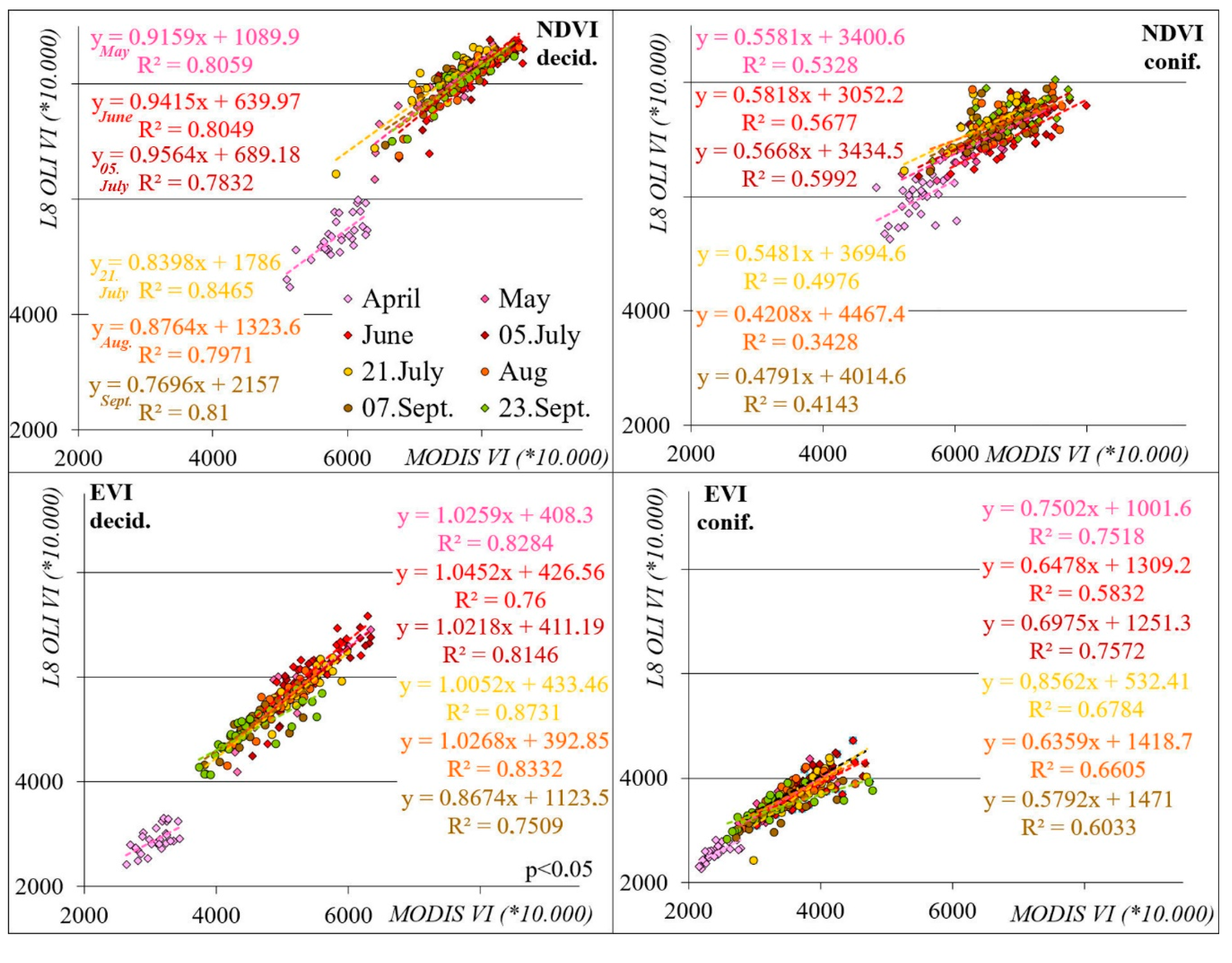
We calculated the linear regressions between MODIS MVC VIs and the LANDSAT OLI-based VI values for eight 16-day periods in the summer of 2015 (Figure 10). The given 16-day composite image was compared with an OLI image recorded on a day of this time period. The deciduous, coniferous, and mixed forests were mapped in cloud-free, corrected OLI images based on CLC 2012. According to the EVI/NDVI median values of the forest areas, the value of the determination coefficient is high between MODIS and OLI, 0.9499 < R2EVI < 0.9926 and 0.88853 < R2NDVI < 0.9753, where the worst values are for the median NDVIconiferuous and the best values are for the median EVIdeciduous. Values for the 30 largest forest patches were compared at each of the eight time periods, where the determination coefficient value ranges already indicated more realistic results, 0.5546 < R2EVI < 0.8731 and 0.2593 < R2NDVI < 0.8465 (Figure 10). Correlation is significant at 95%.
Values for April are well distinguishable in the data series, and here the relation is moderate. Due to the very strong correlation, the changes in the LANDSAT OLI EVI values for deciduous forests in July can be predicted by at least 87% based on the MODIS EVI. EVI and NDVIdeciduous are closely related for the rest of the summer months, 0.77214 < R2NDVI/EVI < 0.8465, but fluctuating, where the values of the NDVI and EVI R2 are higher. According to the relation for deciduous forests, appropriate quality, high-temporal-resolution MODIS data are highly suitable for regional-scale studies.
In the case of pine forest, by comparing MODIS/OLI NDVI and EVI data, the connection is the strongest between EVI values based on the determination coefficients and is more moderate in July only (R2 = 0.7518). Looking at the EVI values for the summer months, the correlation is strong (0.7767 < r < 0.8701). The coniferous forest is characterized by a generally 15% weaker connection with NDVI. The comparative analysis confirms the better usability and accuracy of EVI.
The validation assessment revealed that in general, according to the annually calculated PaDI, NDVI is more accurate, whereas according to OLI, which is calculated using the daily data, EVI is more accurate.
According to Reference [30] the temperature effect can be highlighted considering vegetation development, which is verified by the correlation coefficients between the monthly median temperatures and the MODIS VI medians of different forest types, 0.738 < r < 0.802.
4. Conclusions
The unique feature of our environmental monitoring is the high-temporal-resolution regional analysis, which is achieved via accurate, homogenous surface cover delineation and the highest possible spatial resolution; in this way, MODIS data can be well used for greater scale, regional analyzes. The differences between the results of the deciduous, mixed, and coniferous biomass production indicate complex processes, even within vegetation, which is a factor in the landscape. The complex nature of changes in the underlying 18-year dataset demonstrates the importance of continuous monitoring.
Our study, which analyzed three different woody vegetation types with two types of vegetation indices, shows different processes and produces surprising values and, consequently, we cannot say one index superior is to the other. In the evolution of the productivity values it is evident that, in higher resolution analyzes, other dominant factors in addition to climate have an influence on the vegetation growth.
Overall, the forest biomass production show little trend-like changes in the forest categories (deciduous, coniferous, or mixed), and these are not significant changes due to the length of the time series. As a geographic effect of climate change, the effect of extreme water shortage years/periods can be evaluated with the statistical and spatial visualization of anomalies to support prevention. Changes in one or another sub-period of the entire vegetation period can also be evaluated even in the relatively short, 18-year dataset, such as changes in springtime growing values or the summertime biomass production increase. Via the variability, the rapid response of vegetation to environmental influences can be clearly seen, and forests are vulnerable in short periods. According to climatology predictions, the current short-term biomass production losses could become longer lasting than they are now.
The deviation from the pixel-based average has changed the processes defined in the statistical evaluation in a generally favorable time frame, with the negative deviation affecting large areas. Spatial evaluations can identify where forest interventions are needed.
Due to the complexity of the processes, in aridification studies, it is advisable to aim for synthesis-based practical proposals in which the usage of vegetation monitoring is supported by various free, high-resolution remote sensing database services as well. The extension of the base data and temporal sensitivity increases the data quality of the indices; however, our results also reflect quality improvement in the remote sensing data provision. The spatial and temporal resolution of the methodology and continuous analysis programmed can provide great results for the planning of an operative, near real-time, automatic change detection system in the near future.
Author Contributions
Conceptualization: F.K.; Data management and data processing: A.G.; Methodology: F.K. and A.G.; Investigation: F.K.; Validation: F.K. and A.G.; Visualization: F.K. and A.G.; Writing—original draft: F.K.; Writing—editing: F.K. and A.G.; Funding acquisition: F.K.
Funding
The research has been supported by the Hungarian National Research Fund (OTKA K 124648).
Acknowledgments
This research was supported by the Interreg-IPA Cross-border Cooperation Program Hungary-Serbia and co-financed by the European Union (IPA) under the project HUSRB/1602/11/0057 entitled WATERatRISK (Improvement of drought and excess water monitoring for supporting water management and mitigation of risks related to extreme weather conditions).
Conflicts of Interest
The authors declare no conflict of interest.
References
- Copernicus—Europe’s Eyes on Earth. Available online: https://www.copernicus.eu/en (accessed on 2 July 2019).
- Early Warning and Environmental Monitoring Program (EWEM). Available online: https://earlywarning.usgs.gov/ (accessed on 2 July 2019).
- Burke, M.; Hsiang, S.M.; Miguel, E. Global non-linear effect of temperature on economic production. Nature 2015, 527, 235–239. [Google Scholar] [CrossRef] [PubMed]
- Rakonczai, J.; Fehér, Z. A klímaváltozás szerepe az Alföld talajvízkészleteinek időbeli változásaiban (The role of climate change in the changes of groundwater level in the Great Hungarian Plain). Hidrol. Közl. 2015, 95, 1–15. (In Hungarian) [Google Scholar]
- Newbold, T.; Hudson, L.N.; Arnell, A.P.; Contu, S.; De Palma, A.; Ferrier, S.; Hill, S.L.L.; Hoskins, A.J.; Lysenko, I.; Phillips, H.R.P.; et al. Has land use pushed terrestrial biodiversity beyond the planetary boundary? A global assessment. Science 2016, 353, 288–291. [Google Scholar] [CrossRef] [PubMed]
- Copernicus—High Resolution Layers. Available online: https://land.copernicus.eu/pan-european/high-resolution-layers (accessed on 2 July 2019).
- Mátyás, C. Forecasts needed for retreating forests. Nature 2010, 464, 1271. [Google Scholar] [CrossRef] [PubMed]
- Nemzeti Vidékstratégia 2012–2020 (National Landscape Strategy); Ministry of Agriculture and Rural Development: Budapest, Hungary, 2012; p. 136. Available online: http://www.terport.hu/webfm_send/2767 (accessed on 22 September 2019). (In Hungarian)
- Farkas, J.; Rakonczai, J.; Hoyk, E. Környezeti, gazdasági és társadalmi éghajlati sérülékenység: Esettanulmány a Dél-Alföldről (Environmental, economical and social climate vulnerability: A case study on the Hungarian South Great Plain). Tér Társad. 2015, 29, 149–174. (In Hungarian) [Google Scholar] [CrossRef]
- Copernicus—Corine Land Cover (CLC). Available online: https://land.copernicus.eu/pan-european/corine-land-cover (accessed on 2 July 2019).
- Digital Elevation Model over Europe (EU-DEM). Available online: http://data.europa.eu/euodp/data/dataset/data_eu-dem (accessed on 2 July 2019).
- Verbesselt, J.; Hyndman, R.; Newnham, G.; Culvenor, D. Detecting trend and seasonal changes in satellite image time series. Remote Sens. Environ. 2010, 114, 106–115. [Google Scholar] [CrossRef]
- Xin, Q.; Olofsson, P.; Zhu, Z.; Tan, B.; Woodcock, C.E. Toward near real-time monitoring of forest disturbance by fusion of MODIS and Landsat data. Remote Sens. Environ. 2013, 135, 234–247. [Google Scholar] [CrossRef]
- Lunetta, R.S.; Knight, J.F.; Ediriwickrema, J.; Lyon, J.G.; Worthy, L.D. Land-cover change detection using multi-temporal MODIS NDVI data. Remote Sens. Environ. 2006, 105, 142–154. [Google Scholar] [CrossRef]
- Távérzékelésen Alapuló Erdőállapot Monitorozó Rendszer (Hungarian Forestry Monitoring Based on Remote Sensing, TEMRE). Available online: http://klima.erti.hu/home/erdoallapot-monitoring-2/ (accessed on 2 July 2019). (In Hungarian).
- Kern, A.; Marjanovic, H.; Dobor, L.; Anic, M.; Hlásny, T.; Barcza, Z. Identification of Years with Extreme Vegetation State in Central Europe Based on Remote Sensing and Meteorological Data. South East Eur. For. 2017, 8, 1–20. [Google Scholar] [CrossRef]
- GISS Surface Temperature Analysis (GISTEMP). NASA Goddard Institute for Space Studies. Available online: https://data.giss.nasa.gov/gistemp/ (accessed on 2 July 2019).
- Wilson, R.; Anchukaitis, K.; Briffa, K.R.; Büntgen, U.; Cook, E.; D’Arrigo, R.; Davi, N.; Esper, J.; Frank, D.; Gunnarson, B.; et al. Last millennium northern hemisphere summer temperatures from tree rings. Part I: The long term context. Quat. Sci. Rev. 2016, 134, 1–18. [Google Scholar] [CrossRef]
- Csorba, P.; Blanka, V.; Vass, R.; Nagy, R.; Mezősi, G.; Meyer, B. Hazai tájak működésének veszélyeztetettsége új klímaváltozási előrejelzés alapján (Sensitivity of the Hungarian mesolandscapes according to the modelled climate change). Földr. Közl. 2012, 136, 237–253. (In Hungarian) [Google Scholar]
- Rakonczai, J.; Deák, J.Á.; Ladányi, Z.; Fehér, Z. Indicators of climate change in the landscape: Investigation of the soil—Groundwater—Vegetation connection system in the Great Hungarian Plain. In Review of Climate Change Research Program at the University of Szeged; Rakonczai, J., Ladányi, Z., Eds.; Institute of Geography and Geology: Szeged, Hungary, 2012; pp. 41–59. [Google Scholar]
- Kovács, F.; van Leeuwen, B.; Ladányi, Z.; Rakonczai, J.; Gulácsi, A. Regionális léptékű aszálymonitoringot támogató vegetáció—És talajnedvesség értékelés MODIS adatok alapján (Vegetation and soil moisture assessment based on MODIS data to support regional drought monitoring). Földr. Közl. 2017, 141, 14–29. (In Hungarian) [Google Scholar]
- Lakatos, M.; Bihari, Z.; Szentimrey, T. A klímaváltozás magyarországi jelei (Observed climate change in Hungary). Légkör 2014, 59, 158–163. (In Hungarian) [Google Scholar]
- Bihari, Z.; Babolcsay, G.; Bartholy, J.; Ferenczi, Z.; Kerényi, J.; Haszpra, L.; Újváry, K.; Kovács, T.; Lakatos, M.; Németh, Á.; et al. Éghajlat (Climate). In Magyarország Nemzeti Atlasza 2. Kötet: Természeti Környezet (Hungarian National Atlas, Nature Environment); Kocsis, K., Horváth, G., Keresztesi, Z., Nemerkényi, Z., Eds.; MTA CSFK Földrajztudományi Intézet: Budapest, Hungary, 2018; pp. 58–69. (In Hungarian) [Google Scholar]
- Bartholy, J.; Horányi, A.; Krüzselyi, I.; Pieczka, I.; Pongrácz, R.; Szabó, P.; Szépszó, G.; Torma, C.; Radics, K.; Szentimrey, T.; et al. A várható éghajlatváltozás dinamikus modelleredmények alapján (Expected climate change based on results of dynamic modell). In Klímaváltozás—2011; Bartholy, J., Bozó, L., Haszpra, L., Eds.; MTA-ELTE Meteorológia Tanszék: Budapest, Hungary, 2011; pp. 170–235. (In Hungarian) [Google Scholar]
- Mezősi, G.; Blanka, V.; Ladányi, Z.; Bata, T.; Urdea, P.; Frank, A.; Meyer, B. Expected mid- and long-term changes in drought hazard for the South-Eastern Carpathian Basin. Carpathian J. Earth Environ. Sci. 2016, 11, 355–366. [Google Scholar]
- Integrált Vízháztartási Tájékoztatók (Hungarian Integrated Water Management Bulletin). Available online: http://www.vizugy.hu/index.php?module=documents&programelemid=108 (accessed on 2 July 2019). (In Hungarian).
- Fiala, K.; Blanka, V.; Ladányi, Z.; Szilassi, P.; Benyhe, B.; Dolinaj, D.; Pálfai, I. Drought severity and its effect on agricultural production in the Hungarian-Serbian cross-border area. J. Environ. Geogr. 2014, 7, 43–51. [Google Scholar] [CrossRef]
- Kovács, F. GIS analysis of short and long term hydrogeographical changes on a nature conservation area affected by aridification. Carpathian J. Earth Environ. Sci. 2013, 8, 97–108. [Google Scholar]
- Központi Statisztikai Hivatal (Hungarian Central Statistical Office). Available online: https://www.ksh.hu/docs/hun/xstadat/xstadat_eves/i_uw002.html (accessed on 2 July 2019). (In Hungarian).
- Hunkár, M.; Vincze, E.; Szenyán, I.; Dunkel, Z. Application of phenological observations in agrometeorological models and climate change research. Q. J. Hung. Meteorol. Serv. 2012, 116, 195–209. [Google Scholar]
- Szabó, B.; Vincze, E.; Czúcz, B. Flowering phenological changes in relation to climate change in Hungary. Int. J. Biometeorol. 2016, 60, 1347–1356. [Google Scholar] [CrossRef]
- Czúcz, B.; Molnár, Z.; Horváth, F.; Botta-Dukát, Z. The natural capital index of Hungary. Acta Bot. Hung. 2008, 50 (Suppl. 1), 161–177. [Google Scholar] [CrossRef]
- Pálfai, I. A Duna-Tisza Közi Hátság Vízháztartási Sajátosságai (Peculiarities of water household in Danube-Tisza Interfluve). Hidrol. Közlöny 2010, 90, 40–44. (In Hungarian) [Google Scholar]
- Völgyesi, I. A Homokhátság Felszínalatti Vízháztartása. Vízpótlási és Visszatartási Lehetőségek (Groundwater Household on the Sandy Ridge). In Proceedings of the MHT XXIV, Országos Vándorgyűlés Kiadványa, Pécs, Hungary, 5–6 July 2006; pp. 1–12. (In Hungarian). [Google Scholar]
- Kristóf, D.; Pataki, R.; Neidert, D.; Nagy, Z.; Pintér, K. Integrating temporal and spectral information from low-resolution MODIS and high-resolution optical satellite images: Two Hungarian case studies. In Proceedings of the SPIE—The International Society for Optical Engineering, Florence, Italy, 17–20 September 2007; Volume 6742. [Google Scholar] [CrossRef]
- Solano, R.; Didan, K.; Jacobson, A.; Huete, A. MODIS Vegetation Index User’s Guide; MOD13 Series; Vegetation Index and Phenology Lab., University of Arizona: Tucson, AZ, USA, 2010; p. 42. Available online: https://vip.arizona.edu/documents/MODIS/MODIS_VI_UsersGuide_01_2012.pdf (accessed on 22 September 2019).
- Hmimina, G.; Dufrêne, E.; Pontailler, J.-Y.; Delpierre, N.; Aubinet, M.; Caquet, B.; de Grandcourt, A.; Burban, B.; Flechard, C.; Granier, A.; et al. Evaluation of the potential of MODIS satellite data to predict vegetation phenology in different biomes: An investigation using ground-based NDVI measurements. Remote Sens. Environ. 2013, 132, 145–158. [Google Scholar] [CrossRef]
- Gulácsi, A.; Kovács, F. Drought monitoring with spectral indices calculated from MODIS satellite images in Hungary. J. Environ. Geogr. 2015, 8, 11–19. [Google Scholar] [CrossRef]
- Xie, Y.; Sha, Z.; Yu, M. Remote sensing imagery in vegetation mapping: A review. J. Plant Ecol. 2008, 1, 9–23. [Google Scholar] [CrossRef]
- Huete, A.; Didan, K.; Miura, T.; Rodriguez, E.P.; Gao, X.; Ferreira, L.G. Overview of the radiometric and biophysical performance of the MODIS vegetation indices. Remote Sens. Environ. 2002, 83, 195–213. [Google Scholar] [CrossRef]
- Cuba, N.; Rogan, J.; Christman, Z.; Williams, C.A.; Schneider, L.C.; Lawrence, D.; Millones, M. Modelling dry season deciduousness in Mexican Yucatán forest using MODIS EVI data (2000–2011). GISci. Remote Sens. 2013, 50, 26–49. [Google Scholar] [CrossRef]
- LSDS Science Research and Development (LSRD), USGS. Available online: https://espa.cr.usgs.gov/ (accessed on 2 July 2019).
- Bannari, A.; Morin, D.; Bonn, F.; Huete, A.R. A review of vegetation indices. Remote Sens. Rev. 1995, 13, 95–120. [Google Scholar] [CrossRef]
- Gulácsi, A.; Kovács, F. Drought monitoring of forest vegetation using MODIS-based normalized difference drought index in Hungary. Hung. Geogr. Bull. 2018, 67, 29–42. [Google Scholar] [CrossRef] [Green Version]
- Ahl, D.E.; Stith, T.G.; Sean, N.B.; Nikolay, V.S.; Myneni, R.B.; Knyazikhin, Y. Monitoring spring canopy phenology of a deciduous broadleaf forest using MODIS. Remote Sens. Environ. 2006, 104, 88–95. [Google Scholar] [CrossRef] [Green Version]
- Borgogno-Mondino, E.; Lessio, A.; Gomarasca, M. A fast operative method for NDVI uncertainty estimation and its role in vegetation analysis. Eur. J. Remote Sens. 2016, 49, 137–156. [Google Scholar] [CrossRef]
- Li, Z.; Li, X.; Wei, D.; Xu, X.; Wang, H. An assessment of correlation on MODIS-NDVI and EVI with natural vegetation coverage in Northern Hebei Province, China. Procedia Environ. Sci. 2010, 2, 964–969. [Google Scholar] [CrossRef] [Green Version]
- Szabó, S.; Elemér, L.; Kovács, Z.; Püspöki, Z.; Kertész, Á.; Singh, S.K.; Balázs, B. NDVI dynamics as reflected in climatic variables: Spatial and temporal trends—A case study of Hungary. GISci. Remote Sens. 2019, 56, 624–644. [Google Scholar] [CrossRef]
- Ladányi, Z.; Blanka, V. Relationship of drought and biomass production. In Drought and Water Management in South Hungary and Vojvodina; Blanka, V., Ladányi, Z., Eds.; Department of Physical Geography and Geoinformatics, University of Szeged: Szeged, Hungary, 2014; pp. 132–135. [Google Scholar]
- Kovács, F. Assessment of regional variations in biomass production using satellite image analysis between 1992 and 2004. Trans. GIS 2007, 11, 911–926. [Google Scholar] [CrossRef]
- Szalai, S.; Auer, I.; Hiebl, J.; Milkovich, J.; Radim, T.; Stepanek, P.; Zahradnicek, P.; Bihari, Z.; Lakatos, M.; Szentimrey, T. Climate of the Greater Carpathian Region. Final Technical Report. 2013. Available online: http://www.carpatclim-eu.org (accessed on 22 September 2019).
- Kovács, F. NDVI/EVI monitoring in forest areas to assessment the climate change effects in Hungarian Great Plain from 2000. In Proceedings of the SPIE 10783, Remote Sensing for Agriculture, Ecosystems, and Hydrology XX, 107831H, Berlin, Germany, 10 October 2018. [Google Scholar] [CrossRef]
- Menzel, A.; Sparks, T.H.; Estrella, N.; Koch, E.; Aasa, A.; Agas, R.; Alm-Kübler, K.; Bissolli, P.; Braslavská, O.; Briede, A.; et al. European phenological response to climate change matches the warming pattern. Glob. Chang. Biol. 2006, 12, 1969–1976. [Google Scholar] [CrossRef]
- Hlásny, T.; Barka, I.; Sitková, Z.; Bucha, T.; Konopka, M.; Lukác, M. MODIS-based vegetation index has sufficient sensitivity to indicate stand-level intra-seasonal climatic stress in oak and beech forests. Ann. For. Sci. 2015, 72, 109–125. [Google Scholar] [CrossRef]
Figure 1.
Characterization of forests analyzed on the Danube−Tisza Interfluve in Hungary; based on data: [6,10,11].

Figure 2.
Deviation of the monthly temperature mean (2009–2017) from the 1971–2000 climate normal value in Hungary; based on data [26]. (red: positive deviations, blue: negative deviations).
Figure 2.
Deviation of the monthly temperature mean (2009–2017) from the 1971–2000 climate normal value in Hungary; based on data [26]. (red: positive deviations, blue: negative deviations).

Figure 3.
Proportion of areas affected by drought in Hungary from 1995 to 2018; based on data [29].
Figure 3.
Proportion of areas affected by drought in Hungary from 1995 to 2018; based on data [29].
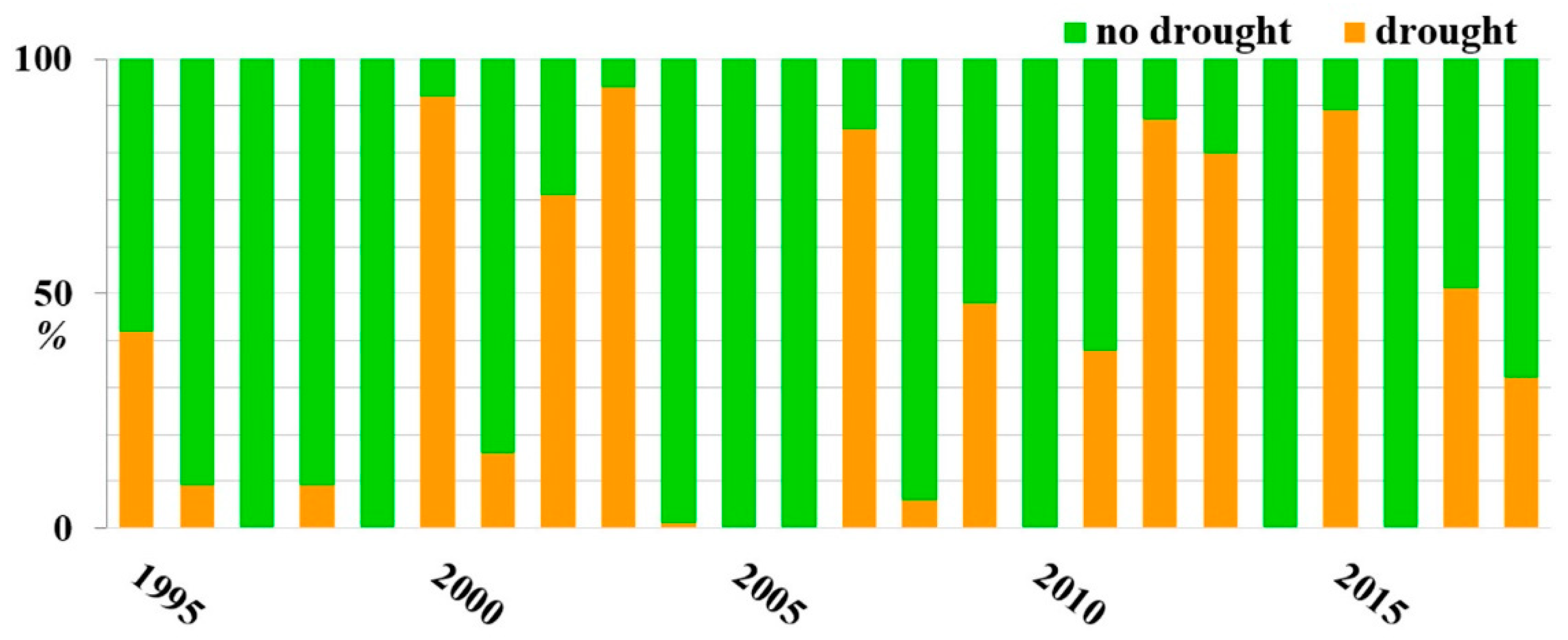
Figure 4.
Deciduous forest EVI data time series based on MODIS MVC images for 16-day periods during the growing season (2000–2017) [52].
Figure 4.
Deciduous forest EVI data time series based on MODIS MVC images for 16-day periods during the growing season (2000–2017) [52].
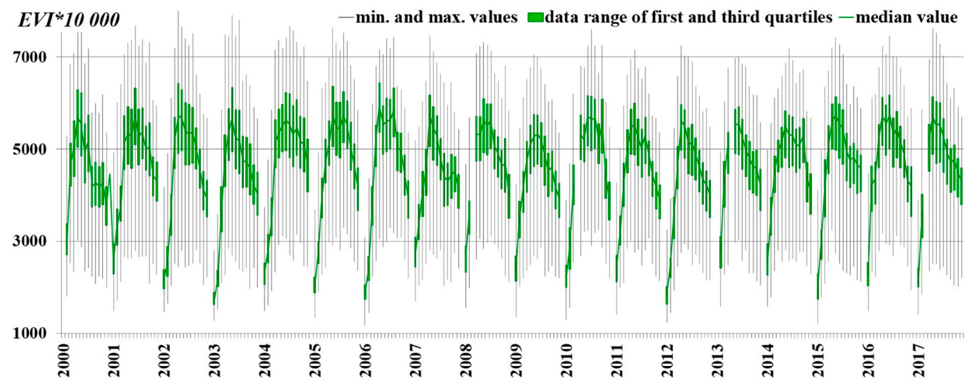
Figure 5.
Deciduous forest EVI median value dataset in the MVC 16-day periods between 2000 and 2017.
Figure 5.
Deciduous forest EVI median value dataset in the MVC 16-day periods between 2000 and 2017.

Figure 6.
EVI yearly standardized deviation of deciduous, mixed and coniferous forests between 2000 and 2017 based on MODIS MVC images.
Figure 6.
EVI yearly standardized deviation of deciduous, mixed and coniferous forests between 2000 and 2017 based on MODIS MVC images.

Figure 7.
Spatiality of EVI standardized deviation for forests in the Danube–Tisza Interfluve between 2000 and 2017 in 250 m spatial resolution MODIS MVC images.
Figure 7.
Spatiality of EVI standardized deviation for forests in the Danube–Tisza Interfluve between 2000 and 2017 in 250 m spatial resolution MODIS MVC images.

Figure 8.
EVI yearly standardized deviation rates for different forest types between 2000 and 2017, based on MODIS MVC images (d: deciduous, c: coniferous, m: mixed forest).
Figure 8.
EVI yearly standardized deviation rates for different forest types between 2000 and 2017, based on MODIS MVC images (d: deciduous, c: coniferous, m: mixed forest).
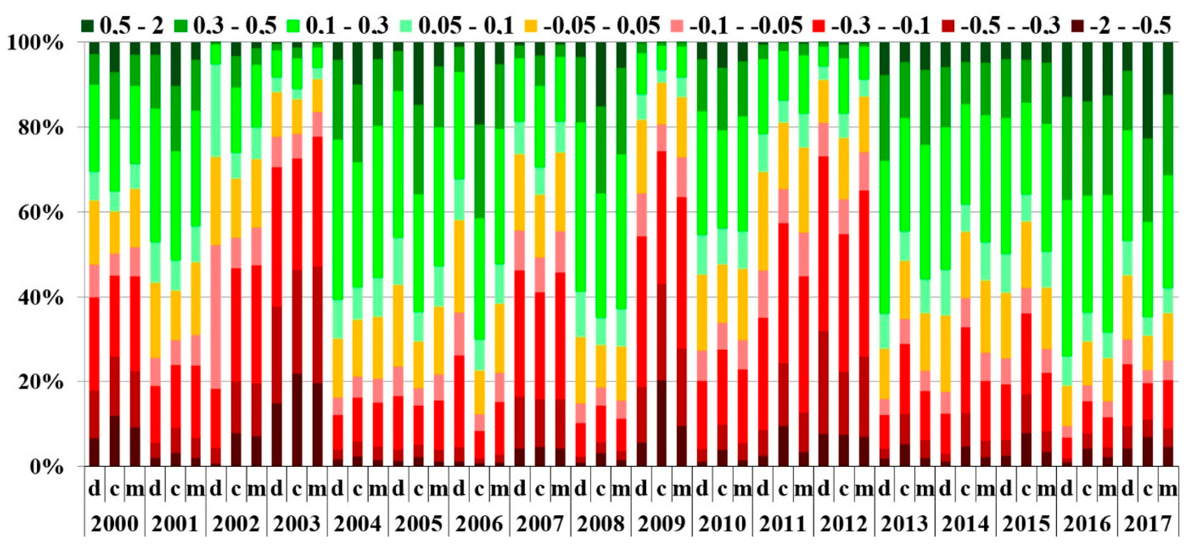
Figure 9.
Determination coefficients between the spectral indices of MODIS images and PaDI for the time period 2000–2010.
Figure 9.
Determination coefficients between the spectral indices of MODIS images and PaDI for the time period 2000–2010.
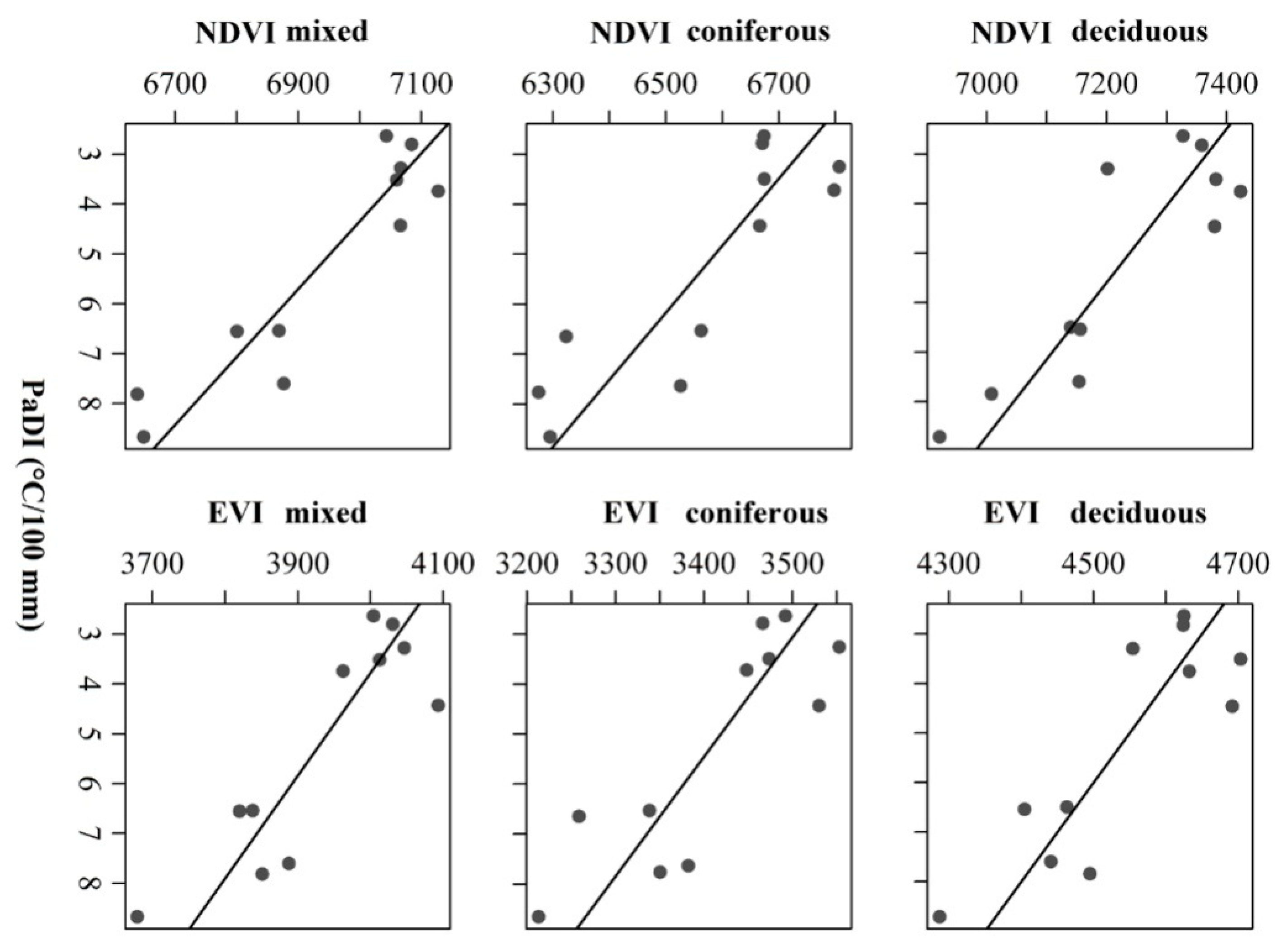
Figure 10.
Evaluation of MODIS 13Q1 NDVI/EVI and OLI NDVI/EVI deciduous and coniferous linear regressions based on the summer semester of 2015.
Figure 10.
Evaluation of MODIS 13Q1 NDVI/EVI and OLI NDVI/EVI deciduous and coniferous linear regressions based on the summer semester of 2015.
© 2019 by the authors. Licensee MDPI, Basel, Switzerland. This article is an open access article distributed under the terms and conditions of the Creative Commons Attribution (CC BY) license (http://creativecommons.org/licenses/by/4.0/).
Share and Cite
MDPI and ACS Style
Kovács, F.; Gulácsi, A. Spectral Index-Based Monitoring (2000–2017) in Lowland Forests to Evaluate the Effects of Climate Change. Geosciences 2019, 9, 411. https://doi.org/10.3390/geosciences9100411
AMA Style
Kovács F, Gulácsi A. Spectral Index-Based Monitoring (2000–2017) in Lowland Forests to Evaluate the Effects of Climate Change. Geosciences. 2019; 9(10):411. https://doi.org/10.3390/geosciences9100411
Chicago/Turabian StyleKovács, Ferenc, and András Gulácsi. 2019. "Spectral Index-Based Monitoring (2000–2017) in Lowland Forests to Evaluate the Effects of Climate Change" Geosciences 9, no. 10: 411. https://doi.org/10.3390/geosciences9100411
Note that from the first issue of 2016, this journal uses article numbers instead of page numbers. See further details here.