Modeling the Natural Drainage Network of the Grand River in Southern Ontario: Agriculture May Increase Total Channel Length of Low-Order Streams

1
Department of Chemistry and Biology, Ryerson University, 350 Victoria Street, Toronto, ON M5B 2K3, Canada
2
Environmental Applied Science and Management, Ryerson University, 350 Victoria Street, Toronto, ON M5B 2K3, Canada
*
Author to whom correspondence should be addressed.
Geosciences 2019, 9(1), 46; https://doi.org/10.3390/geosciences9010046
Submission received: 5 December 2018
/
Revised: 29 December 2018
/
Accepted: 10 January 2019
/
Published: 17 January 2019
(This article belongs to the Special Issue Hydrology in River Basins: Developments in Science and Application (HRBDSA))
Abstract
:The Grand River watershed is an important agricultural area in southern Ontario, with several large and growing municipalities. Based on digital elevation models (DEMs), the natural drainage network was modelled to predict flow paths. Channel lengths and locations of the predicted network were compared with a ground-truthed channel network to determine efficacy of the models. Approximately 5% of predicted channels lay >40 m from actual channel locations. This amounted to 388 km of channel that had no corresponding channels in reality. The model was unable to predict, based on topography, 2535 km of actual channel present in the watershed. Channels not anticipated by topography were mostly first-order, with low sinuosity, were most common in areas with high agricultural land use, and are likely excavated extensions to headwater streams to facilitate drainage. In addition, this study showed that Soil and Water Assessment Tool (SWAT) models produced using different DEM resolutions did not predict significantly different stream flows, even when resolution was as low as 200 m. However, these low resolution DEMs did result in under-prediction of sediment export entering Lake Erie, most likely because the low resolution maps failed to account for small localized areas of high slope that would have relatively higher rates of erosion.
1. Introduction
Engineering of stream channels generally occurs within a context of broader changes in land use. Between one-third to one-half of the land surface has been modified by human activities [1]. Land conversion to more economic uses (in a conventional sense of financial benefit to landowner) has been a chief component of economic growth; many land use and land cover changes are set in motion by individual landowners and land managers [2]. Much engineering of stream channels has coincided with clearing of land for agriculture, launching the agrarian economy of the nineteenth and early twentieth century in the United States and Canada.
While land use conversion continues, the rate of conversion peaked in Canada in the late 19th century. Globally, land modification will continue to increase with a growing population, its demand for food, and urban development [3]. Conversion of land has many social, economic, and environmental ramifications which are acknowledged, but which lay beyond the scope of this paper.
Channelization can reduce the length of a meandering stream, replacing it with a straightened course with sometimes drastically altered channel width, depth and bank slopes. Channelized headwater streams increase flow carrying capacity and flow velocity, both of which result in ecological disturbances. Collateral effects of channelizing streams include removal of riparian vegetation, removal of in-stream substrate, an increase in bed gradient, reduced transient storage capacity, and a decrease in total network length of headwater streams. Removal of riparian vegetation and in-stream bottom substrate, coupled with the greater flow capacity, increase bank and bed erosion, leading to higher suspended sediment loads and sediment export from the watershed [4,5]. Streams originating in agricultural landscapes not only experience altered flow regimes and increased transport of sediment, but increased nutrient transport, contributing to cultural eutrophication in receiving water bodies [6]. Headwater streams are particularly important in processing and retaining nutrients; however, the nutrient retention capacity is compromised by increased depth [7] and reduced transient hydrologic retention associated with channelization [8,9]. Farmers dislike losing soil to the erosive forces of streams, and generally would rather not be under scrutiny by environmental regulators for contributing to nutrient export and eutrophication. However, steam channelization offers the trade-off of effective drainage and enhanced crop growth in wet soils. As a result, reaches that were channelized in the past are often maintained, and in jurisdictions with weak environmental regulation and continued land use conversion, sinuous reaches are straightened.
The primary purpose of this research was to investigate the impact of landuse on stream network in the Grand River Watershed (GRW) in Southwestern Ontario. This is an important agricultural region of Ontario, and row crop agriculture is the predominant land use in the basin. The drainage network of the GRW was constructed, based on soil layers and topography, to serve as a null model for comparison against the existing drainage network. This provided an opportunity to consider how channel engineering associated with land use (primarily agriculture) has affected drainage density, total channel length, and sinuosity in the network. Moreover, we need to have a good understanding of the strengths and limitations of the dataset and the modeling approaches since these tools will be used for remediation, watershed restoration and other important decision-making processes such as funding, grants and resource allocation within the watershed. Furthermore, similar watersheds in Ontario have experienced the same fate at the GRW and what is learned from this study may directly benefit the surrounding watersheds in southern Ontario.
Watersheds have emerged as the basic unit for most hydrologic analyses. Manual survey of a watershed can be expensive and time consuming. However, geographic information systems (GIS) have become valuable investigative tools with respect to stream visualization and analysis. With GIS, one can add spatial elements and also perform analysis of variables such as slope, aspect and other watershed parameters including climate, topography, soil type, vegetative cover, population density, point source of pollution and farming practice. With GIS, it is possible to greatly reduce processing time (as compared to field surveys) and elements of subjectivity that are frequently encountered with the manual measurement of features on maps and aerial photographs. When large watersheds are being studied, digital data resolution is important since digital elevation models (DEMs) are the primary topographic inputs of hydrologic modelling. A digital elevation model is a numerical representation of a surface that represents the height of the terrain. According to Ariza-Villaverde et al. [10], a DEM may be considered in different ways, such as by (a) contours with x, y coordinate pairs along each contour line of a specified elevation, (b) a triangulated, irregular network made up of nodes that are irregularly distributed and lines with 3-D coordinates (x, y, z) and (c) a 2-D array of numbers that represents the spatial distribution of elevations on a regular grid. The latter model is widely used for raster DEMs. Previous studies [10,11,12,13,14,15] have examined the effect of spatial resolution on modeling and quantifying stream networks in watersheds of varying sizes and have concluded that the distance between actual stream networks and DEM derived stream networks increase exponentially at higher resolutions. However, none of these studies specifically examined the effect of different resolutions on headwater streams or on stream sinuosity.
The algorithm in GIS software is commonly employed as an eight-direction (D8) flow model in order to derive hydrologic characteristics of a surface such as the direction of flow from every cell in the raster [10,12]. In this model, there are eight valid output directions in relation to the eight surrounding cells into which flow can enter. The direction of flow is then computed from the direction of steepest descent and the process is repeated to produce higher order streams in the stream network. Immediately, two limitations of the D8 technique stand out: it will not function as anticipated on flat terrains, and secondly, aquatic features such as lakes may not be delineated or accounted for. One possible workaround is to burn the stream network onto the DEM to account for streams on flat terrains.
Thus, a secondary objective of this research was to consider the effect of spatial resolution in DEMs on prediction of stream networks, and modeling of hydrology and sediment export from the GRW.
2. The Grand River Basin, Southern Ontario
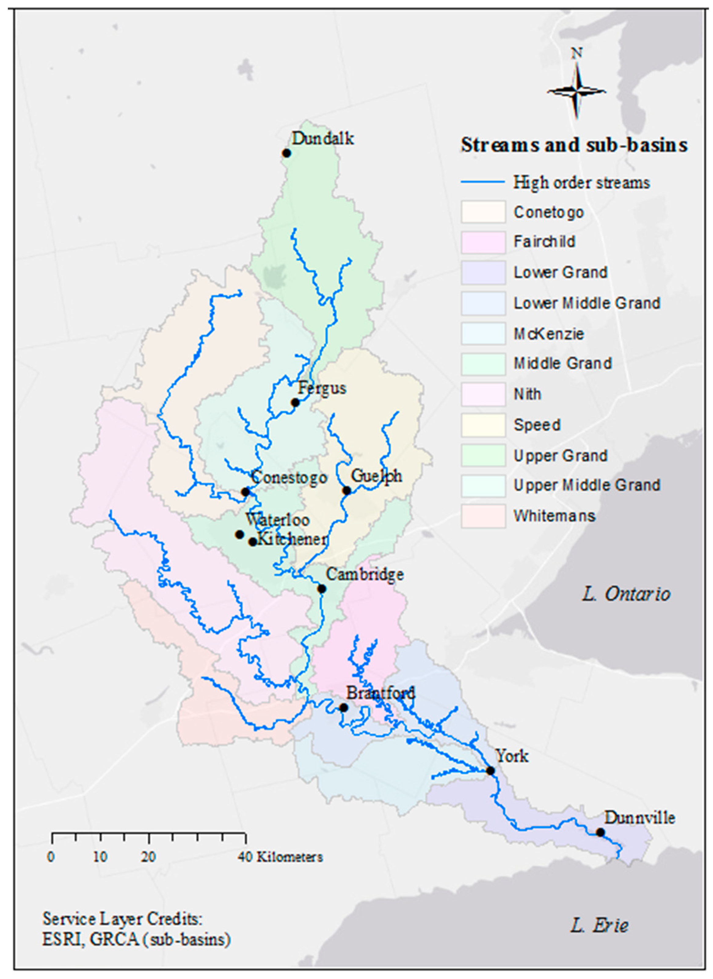
The Grand River Watershed covers an area of 6965 km2 and it is the largest of the watersheds in Southwestern Ontario that drain into Lake Erie (Figure 1). Spanning a length of 290 km and having an elevation differential of about 362 m from source to mouth, the Grand River follows a dendritic pattern after it originates at the Dundalk Highlands, flows through Port Maitland and contributes about 10% of the drainage to Lake Erie [16].
Prior to the arrival of Europeans around the mid-1770s, First Nations inhabited the basin which was dominated by pristine forests, marshes and swamps. From the 1750s, wetlands and forests in the GRW have been progressively modified to make way for lumber exploitation, agriculture, pasture, settlements and industry. Nearly 95% of historical forest has been removed and there has been extensive stream engineering of the waterscapes [16], especially by damming and channelization [17]. By the early 1900s, almost 70% of all drained wetlands in southern Ontario were converted into agricultural lands, with noticeable degradation in water quality. In 1934, the Grand River Commission received its charter, tasked with finding a solution to the degradation in stream flows and water quality [16]. With around 6000 farms, agriculture has remained the dominant land use in the GRW [17]. Approximately 82% of land on the upper Grand (e.g., Nith and Conestogo sub-basins) is in agriculture as compared to ~64% in the central Grand. At present, forests and wetlands occupy around 20% of the total watershed [18]. Row crops, small grains, forage and bare agricultural fields accounted for 20.5%, 12.1%, 19.2% and 15.9% of the GRW, respectively. The GRW has some of the fastest growing urban centres in Canada. Just over one million people live in the GRW, with 81% residing on 7% of the land area in Kitchener, Waterloo, Cambridge, Guelph and Brantford [17].
A 1982 Grand River Basin Water Management Study identified intensive agriculture as the main nonpoint source of pollution responsible for impairment of water quality in the Grand River [19]. Based on the Water Quality Index used by the Canadian Council of Ministries of the Environment, the headwaters of the Grand River are classified as ‘good’; however, as tributaries flow through major agricultural areas, their status drops to ‘fair’; and finally, as larger tributaries and the main Grand River flow past urban centres, water quality drops to ‘poor’ due to the addition of high levels of phosphorus and nitrogen from storm water and sewage treatment plants [16].
3. Methods
3.1. Stream Delineation
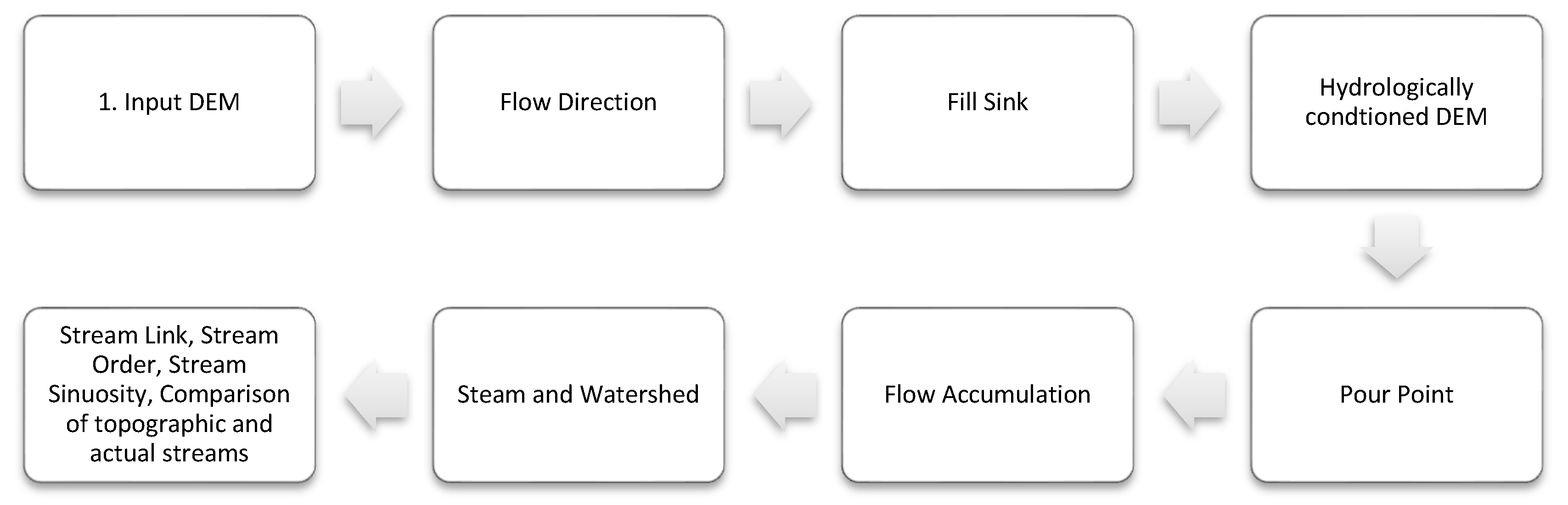
ESRI’s ArcMap 10.2 Hydrology tool (ESRI, Redlands, CA, USA) was used to delineate the Grand River watershed using a preprocessed digital elevation model (DEM) at 10-, 25- and 200-m spatial resolutions. The main steps that were followed are: hydrological conditioning, watershed delineation, and derivation of stream network characteristics. A flowchart for the procedure is as follows (Figure 2):
Comparisons of distances and lengths of the DEM-derived streams (target layer) and the ground-truthed reference stream network were run at spatial queries of 0, 2.5, 5, 10, 20 and 40 m to evaluate the extent of overlap between the two stream networks.
A shapefile containing the different sub-basins within the GRW (downloaded from https://data.grandriver.ca/downloads-geospatial.html) was used to clip sub-basins in the DEM derived watersheds, soil (downloaded from Land Information Ontario: https://www.ontario.ca/page/land-information-ontario), tile drainage (downloaded from the Ontario Ministry of Agriculture, Food, and Rural Affairs: https://www.ontario.ca/page/land-information-ontario), and land cover (downloaded from Grand River Conservation Authority: https://data.grandriver.ca/downloads-geospatial.html) layers. Analyses were performed on each sub-basin to determine land use, soil drainage and type, tile drainage area, stream length, order and reach sinuosity. Sinuosity is the extent of curving and is a quantitative measure of reach meandering. Stream sinuosity is calculated as a ratio of the actual reach length to its straight-line distance between two points at 100 m intervals on the reaches.
3.2. Effects of DEM on SWAT Model Performance
A Soil and Water Assessment Tool (SWAT) model has been recently developed for the Grand River Basin. This model is described, along with calibration and validation for the prediction of discharge and export of sediments and nutrients from the GRW [20]. Because it is a physically-based model, SWAT provides the unique opportunity to simulate the hydrology and water quality of ungauged streams and to quantify the relative impacts of alternative input data on hydrology and water quality in watersheds. In the model developed for the GRW, a DEM with 10-m resolution was used for the delineation of the Grand River Basin, sub-basins, hydrologic response units (HRUs), and for identification of pour points from the watershed overall, from each sub-basin, and HRU. This model’s layers for sub-basins, HRUs and pour points were overlaid with the actual stream network, so the 10-m DEM was not used to predict the channel network, as was described above. The hydrologic response unit (HRU) is the smallest spatial unit in the SWAT model and this unit represents areas irrespective of size with similar land uses, soils, and slopes within a sub-basin based upon user-defined thresholds. This method makes for an effective approach in discretizing large watersheds where simulation at the field scale may not be computationally feasible [21].
The availability of a ground-truthed digital river network, and of a 10-m resolution DEM for the GRW, is a luxury. Not all watersheds for which one might wish to build a SWAT model have either available. It is not clear how strongly the use of a lower resolution elevation model may affect the quality of the SWAT model, particularly if the DEMs must be used not only to predict topographical features (e.g., HRUs), but also to predict the channel network. In the current study, the effects of DEM resolution on SWAT model predictions for hydrology and sediment transport were evaluated by delineating the stream network, the basin, sub-basin, and pour points using 10-m, 25-m, and 200-m resolution DEMs. As the SWAT model, constructed using a 10-m resolution DEM with an actual stream network layer, has been calibrated and validated with respect to predicting discharge and sediment load, it serves as the comparator against which performance of SWAT models, built using DEMs of varying resolution, can be assessed.
3.2.1. Preparation of SWAT Model Input Data
A DEM (10 × 10 m resolution) for Ontario was obtained via the Scholars Geospatial Portal at Ryerson University (http://geo2.scholarsportal.info/). This DEM (version 2.0.0) is a 3-D raster data set which captures terrain elevations and has cell resolutions of 10 m in southern Ontario. A rectangular clipped portion of the DEM was used to delineate the watershed and the pour point was snapped on the main stream network as it entered Lake Erie. The GRCA’s ground-truthed stream network (https://data.grandriver.ca/downloads-geospatial.html) was burned onto the raster during the watershed delineation process to produce more accurate sub-basin delineations in subsequent steps. The virtual stream layer is a single line, fully connected network that represents the inferred flow through watercourses and water bodies. DEMs with lower resolution (25- and 200-m) were also obtained from GRCAs website (https://data.grandriver.ca/downloads-geospatial.html).
The primary DEM used in this study was based on the Provincial Digital Elevation Model (Ontario’s PDEM) that most closely reflects true ground elevations as much as possible. The raster was constructed using several data sources to provide seamless coverage for all of Ontario. These data sources include the Ontario Basic Mapping (OBM) program and NASA’s Shuttle Radar Topographic Mission (SRTM) including the Ontario Radar Digital Surface Model (ORDSM), OBM DTM, OBM Spot Height and OBM Contour. A number of interpolation techniques were employed including: ANUDEM/ESRI Topogrid spline interpolation, ESRI Local Polynomial Interpolation (LPI) algorithm for areas covered by SRTM, and ESRI Bilinear Resampling of finer resolution DTM’s derived from more recent high resolution elevation data acquisitions. Data for the final DEM product was captured at a scale of 1:10,000, with an absolute Positional Accuracy of 5 m and absolute Vertical Accuracy (contours and DTM) of 2.5 m.
3.2.2. Land Cover/Land Use
Land cover classification was based on Landsat 7 TM Imagery in 1999 and updated in 2005 (downloaded from Grand River Conservation Authority: https://data.grandriver.ca/downloads-geospatial.html). Pixel sizes in the landcover GRID were 25 m × 25 m. To date, SWAT has a library of 97 plant types and 8 urban land uses in its database. The GRW was divided into 19 of these different land cover categories, listed here along with corresponding SWAT code in parentheses: built-up (residential) (URHD), built-up (commercial/industrial) (UCOM), row crops (AGRR), small grains (AGRL), forage (ALFA), pasture/sparse forest (PAST), dense forest (deciduous) (FRSD), dense forest (conifer) (FRSE), dense forest (mixed) (FRST), plantation (mature) (AGRL), open water (WATR), wetlands (WETL), extraction/bedrock/roads/beaches (BARR), golf courses (FESC) and bare agricultural fields (AGRL).
3.2.3. Soil Classification
Geospatial data were obtained from the Soil Landscapes of Canada’s online geospatial database that is maintained by the Canadian Soil Information Service or CanSIS (http://sis.agr.gc.ca/cansis/). A soil database was built to identify and link the physiochemical properties of the top 10 layers (if present) of the soil profile to the soil groups in the watershed. The names and characteristics of the different soil layers were also downloaded from the CanSIS website in the Soil Name Table and the Soil Layer Table. SWAT requires the following properties for each layer within the soil: soil hydrologic group, maximum rooting depth of soil profile, fraction of porosity from which anions are excluded, maximum crack volume of soil profile, texture of soil layer, depth from soil surface to bottom of layer, moist bulk density, available water capacity of the soil layer, saturated hydraulic conductivity, organic carbon content, clay content, silt content, sand content, rock fragment content, moist soil albedo, USLE K, electrical conductivity, soil CaCO3 and soil pH. This database was then appended to the SWAT usersoil database.
Soil slope was divided into four groups based on a modification of the Canada Slope Gradients classification: little or no slope (0–3% gradient), gentle slope (3–9% gradient), moderate slope (9–15% gradient) and steep or excessively steep slope (>15% gradient). After the watershed was delineated, SWAT generated HRUs by overlaying and combining land use, soil and slope.
3.2.4. Weather Data
Daily maximum and minimum (°C), precipitation (mm·d−1), wind speed (m·s−1), solar radiation (MJ·m−2) and relative humidity (fractional) are required weather inputs provided for the length of SWAT run (31 years in total). Weather data were assigned to every sub-basin using data from the station that is closest to the centroid of that sub-basin. All weather data were obtained from Environment Canada (http://climate.weather.gc.ca/historical_data/search_historic_data_e.html) and missing data downloaded from the SWAT’s Global Weather Data tool (http://globalweather.tamu.edu/). Also, due to absence of measured some daily solar radiation, humidity and wind speed datasets, the Hargreaves’ method of simulating potential evapotranspiration was selected for the model run. This method of inferring PET rates has shown reliable estimates when compared to measured values [22,23]. The use of simulated weather data to fill the missing gaps on streamflow using SWAT is modelled in many environments [24,25].
3.2.5. SWAT Model Construction and Run
The duration of the SWAT run was set up from 1980 to 2010 and the model was run on a monthly time scale using a 10/10/10 Multiple HRU threshold for soils, land use and slope. The model was run on a monthly scale for four different scenarios: (a) 10-m DEM using the ground-truthed stream network (referred to as a comparator), (b) 10-m DEM using ArcSWAT for stream delineation, (c) 25-m DEM using ArcSWAT for stream delineation and (d) 200-m DEM using ArcSWAT for stream delineation. Manual calibration of streamflow and sediment discharge was done using parameters as outlined in a SWAT model for the GRW that has been constructed, calibrated, and validated for prediction of water discharge, sediment transport and phosphorus transport [20].
4. Results and Discussion
4.1. Stream Network Delineation
The quality of predicted stream networks, based on DEMs at 10 m and 25 m resolution, was assessed by comparing the total channel length predicted by these models versus the actual channel length in the GRW network, and by determining how well the predicted stream channels spatially coincided with actual stream channels. The total stream length for the GRW network in the reference network source layer is 11,329 km. The stream network derived from the 10-m and 25-m resolution DEMs predicted similar total stream lengths of 9182 km and 8958 km, respectively, or 81.0% and 79.1% of the actual total stream length. Hence, approximately 20% of the stream network cannot be topographically derived. The actual stream network has greater total stream channel density than the predicted network derived from either DEM, as illustrated by comparing the actual network versus that predicted from the 10-m resolution DEM (Figure 3A).
Spatial agreement between predicted stream networks and the actual GRW network was considered based upon how much of the total predicted channel length lies within various distances of actual stream channels. Of the total 9182 km of channel length predicted from the 10-m resolution DEM, 8102 km, or 88.2%, overlapped with actual channel positions (Table 1), while 8325 km or 90.7% of the total length of predicted channels lie with 5 m of actual channel positions. The 25-m resolution DEM was also useful in predicting channel position, with 7818 km of the total predicted network overlapping with actual channel positions. However, the 10-m resolution DEM provided a better correspondence to the actual network, as 95% of the total predicted channel length fell within 17 m of actual channel positions, while 95% of predicted channel length fell within 40 m of actual channel positions for the network derived using the 25-m resolution DEM.
Approximately 48% of the total channel length in the GRW network is first-order, with an additional 23% being second-order (Figure 4), consistent with the distribution in basins described elsewhere [26,27]. Predicted network models based on DEMs were good at predicting the positions of channels second-order or higher, but were less accurate in predicting positions of first-order channels. If one considers only those predicted channels that did not lie within 10 m of existing channels, one would expect 48% of the total length to be represented by first-order streams. This would be true if the model predicted positions of all channels equally well regardless of size (stream order). Similarly, one would predict 23% of the total length of these outlying channels to be second-order. However, when considering only those predicted channels that fail to lie within 10 m of actual channels, 82% and 76% of the total basin-wide channel length are first-order in networks derived from the 10-m and 25-m resolution DEMs, respectively (Table 2). In contrast, 16% and 17% of the predicted channels that do not lie within 10 m are second-order for networks derived from 10-m and 25-m resolution DEMs. The findings of this section is in agreement with previous studies that show that as DEM resolution decrease, the overlapping distances exponentially increases at resolutions greater than 180 m [10,11,12,13,28].
Stream networks predicted by DEM models include some channels that do not exist in reality. These missing channels (or sub-networks) may be a result of a variety of factors, such as burial in the course of urban development. In contrast, predicted networks were missing some channels that do exist in reality. Upon closer inspection of these missing channels, many were relatively straight headwater channels, extending upstream of their predicted starting locations based on DEMs (Figure 3B). The sinuosity of these channels was very low at ≤1.06 km channel length per linear km (Table 2). Channelization, or straightening of meandering reaches of streams, is a common practice in agricultural areas, but contrary to expectations, there is little evidence that this type of modification has occurred to a substantial degree in the GRW. Actual total network channel length is greater than that predicted from topography, and sinuosity in all major sub-basins, and for the network overall, was greater than sinuosity predicted from DEMs (Table 3). Though the D8 method of flow accumulation (and indirectly, stream length) may account for some of these systematic differences [10,12], it alone cannot account for such large discrepancy since most of the unaccounted streams are in the headwaters where topography is not an issue with flow direction and flow accumulation using the D8 method. The only logical variable that would most likely account for such observed difference is the highly agricultural nature of the land and its subsequent modification of the landscape.
The stream network density for a drainage basin is widely used as the starting point for stream restoration [29]. Comparing predicted versus actual network density can indicate areas where restoration efforts might be focused on increasing channel length, or where regulatory actions might be indicated to protect further loss of stream network density. Interestingly, in the GRW, it appears that land use modifications may marginally increase, rather than decrease, total channel length and stream network density. Possibly, this is a result of extending headwater streams as channels or ditches to increase drainage from agricultural lands. Sub-basins of the GRW differ in land use, with percent of land in agricultural production varying from 43.4% (Middle Grand) to 78.0% (Conestogo River) (Table 3). The percentage of total stream network that is first-order also varied among sub-basins, and was correlated with percent agriculture (r = 0.61, p = 0.04). Extending headwater streams for drainage from agricultural lands may contribute to this pattern, although the circumstantial concentration of agricultural activity in the northern portion of the GRW, the headwaters of the basin, likely contributes more to the relationship. However, the difference between DEM-predicted and actual % first-order stream length ([% predicted–% actual]/% actual) is also correlated with percent agricultural activity across sub-basins (r = 0.70, p = 0.015), suggesting that the extension of headwater streams for agricultural purposes has a pervasive effect on the GRW channel network.
Headwaters are important lotic systems that represent hydrological connectivity [30] between upland and downstream waters [31] by facilitated transferal of mass, momentum, energy, or biota within or between various components of the hydrologic cycle [32]. Whether perennial or intermittent, headwater streams are important sites for biogeochemical transformation of nutrients [33]. Due to their dendritic, hierarchical patterns and their large width to depth ratio, headwater streams are critical in controlling the amount of nutrients that are exported downstream [34]. It is the dynamic coupling of hydrological and biogeochemical processes in headwaters that regulates not only the chemical form of the nutrient that is being transported, but also its residence time and longitudinal transport to downstream receiving waters with the fastest uptake and subsequent transformation of nitrogen takes place in headwater streams.
Land use changes do impact hydrology and hydrological processes [35]. The Grand River basin is highly agricultural. The apparent increase in first-order channel length by extending headwaters to facilitate drainage may mitigate some of the impacts of agricultural runoff on the Grand River. This notwithstanding, the Grand River is consistently rated poor with respect to water quality prior to entering Lake Erie.
These extended reaches of headwater channels provide a unique opportunity for land owners, the conservation authority, municipalities and other stakeholders, to target effective stream restoration polices and agricultural best management processes within major basins in the watershed, particularly in those with especially high agricultural activity such as Conestogo, Nith and Upper Middle Grand, in an effort to abate sediment and nutrient export into Lake Erie. Restoration activities might be concentrated on these extended reaches (effectively ditches) to improve sediment and nutrient retention and processing near the site of loading. Such activities come at cost, and it is important to first define what impact such targeted efforts in these relatively small stretches of the watershed might have on water quality. Recently, a SWAT model for the GRW was constructed, calibrated, and validated for prediction of water discharge, sediment transport, and phosphorus transport [20]. This model can provide an effective tool for future testing of the application of Best Management Practices to these extended headwater channels, to reduce sediment and nutrient transport. This would provide some guidance on how best to balance management goals and objectives with costs of implementation. This, as well as full discussion of the SWAT model, are beyond the scope of the current study, however the SWAT model for the GRW was developed using the 10-m DEM to generate the predicted channel network. As this paper considered the effects of DEM resolution on predictive fidelity to the true network, the effects of DEM resolution on SWAT model are considered next.
4.2. Effects of DEM Resolution on SWAT Model
The resolution of the DEM used had varying impacts on the delineated watersheds with respect to watershed sizes, sub-basin number and sizes, and HRU number and sizes (Table 4). The use of a 10-m DEM to generate stream channel networks, and to delineate basins, sub-basins, and HRUs produced a larger watershed with fewer sub-basins but more HRUs relative to the SWAT model using a 10-m DEM, but with the actual stream network layer. The number of sub-basins and HRUs delineated, as well as predicted watershed area decreased with DEM resolution. The SWAT model using the 200-m DEM delineated 92% of the total number of sub-basins (based on comparator model), however it only delineated 60% as many HRUs. This difference in number of HRUs may result in loss of important information on watershed heterogeneity and may affect SWAT outputs such as stream flow, sediment and nutrient yields.
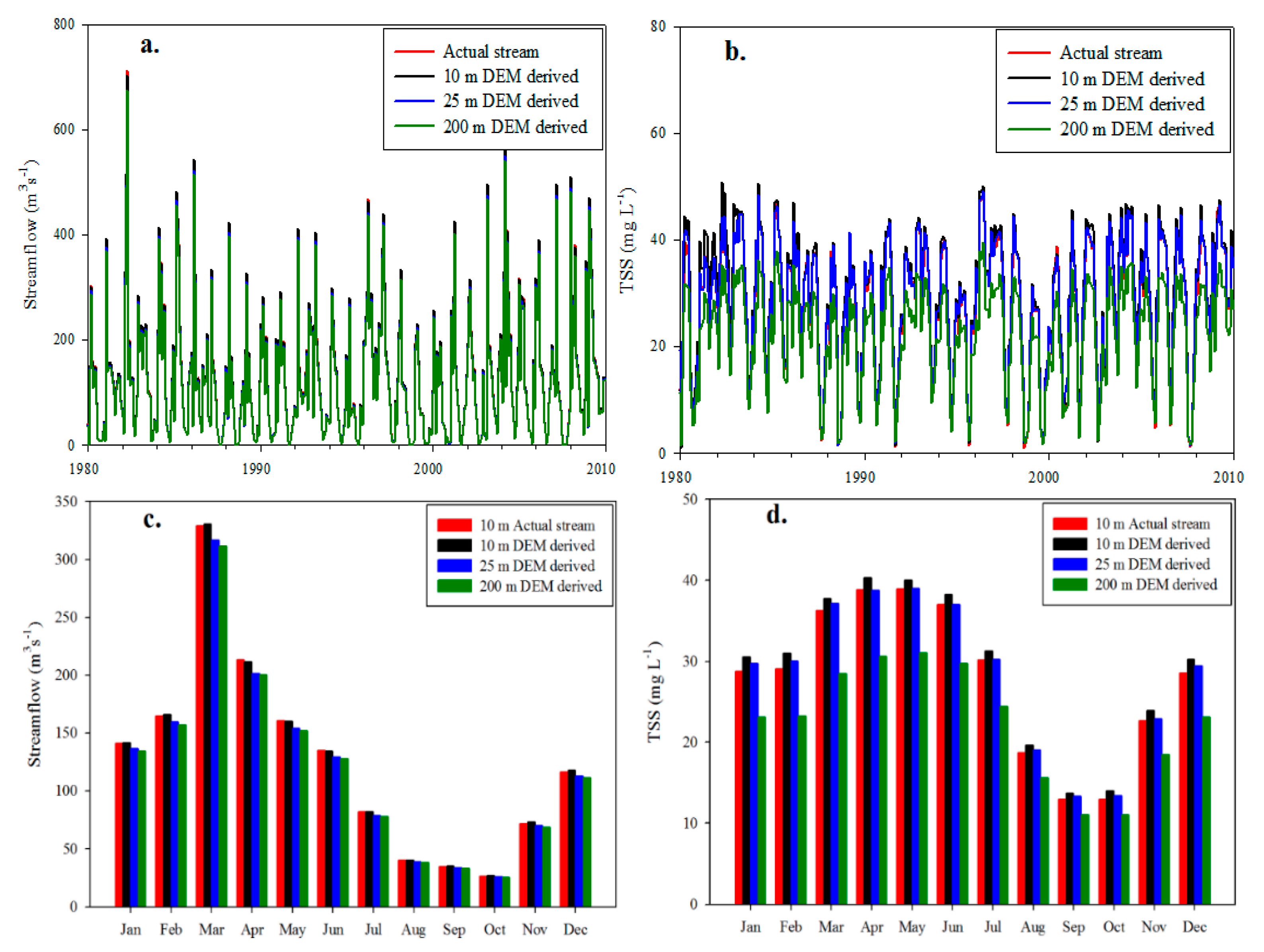
SWAT models built with lower resolution DEMs had lower predicted discharge and sediment export (Table 4). However, all models performed well in predicting discharge, agreeing to within ~5% of the comparator model. This agreement held over 10 years of the model simulation (Figure 5a), and for monthly averages across all years (Figure 5b). By default, the SWAT model mainly estimates watershed runoff using the Soil Conservation Service (SCS) runoff equation. The runoff curve number (CN) is an empirical parameter that predicts surface runoff and infiltration rates from a rainfall event in a particular area. CN is essentially a coefficient that reduces the total precipitation to runoff potential, after accounting for evapotranspiration, infiltration and surface storage. CN is highly dependent on the hydrologic soil group and land use and to a lesser extent, treatment and hydrologic condition. Although DEM reflects topography and slope, these are not the primary variables that influence runoff, hence, differences in DEM resolution resulted in negligible differences in monthly stream flow into Lake Erie from the Grand River watershed.
The models using 10-m and 25-m spatial resolution also agreed well with the comparator model for sediment export, again to within 5%. These models generally overpredicted TSS export. This was true across years, but the overestimate in TSS export was most observed in years with high discharge such as in the early 1980s (Figure 5c), and similarly in spring months with high discharge (Figure 5d). The SWAT model constructed using 200-m spatial resolution under predicted sediment export, by ~20% relative to the comparator model. This was consistent across years, and was also most pronounced in spring months when discharge was highest. SWAT uses the Modified Universal Soil Loss Equation (MUSLE) to estimate soil loss from sub-basins. MUSLE depends on the slope-length gradient which in turn depends on slope length and slope steepness, both of which are determined from the DEM base layer. Based on SWAT’s watershed delineation and subsequent MUSLE calculation, slopes were higher and slope lengths were shorter for higher resolution DEMs when compared to coarser resolution. Consequently, the SWAT model using low resolution DEM recognized little heterogeneity in slope within HRUs, missing local but relatively small areas of high slope which contribute to greater erosion.
5. Conclusions
- The DEM resolution is important in predicting the extent of a river network and the location of stream channels. The use of a DEM with 10-m resolution did a better job in simulating the actual river network than DEMs of lower resolution.
- The existing river network includes first order channels that are not predicted from topography. Perhaps this is a function of resolution and 10-m is too coarse to predict the upper limits of first order channels with fidelity. Or, perhaps these reflect an extension of headwater channels to serve in drainage from agricultural areas. This is supported by the low sinuosity of these unpredicted portions of headwater streams, sinuosity being less for these reaches then for first order streams overall in the sub-watersheds. Also supporting this is the relationship between agricultural activity and the percent of the channel network that is comprised of first order streams, as extension of headwater channels for drainage would increase the overall percent of a network that is first-order. Moreover, the relationship between agricultural activity and the percent difference between actual and predicted first-order streams suggests that there are more unaccounted for kilometers of first-order streams in more agricultural sub-basins.
- DEM resolution is less important in predicting river network hydrology, as there was little difference in output of SWAT models using 10-m, 25-m, or 200-m resolution. Predicted discharge was similar among models regardless of resolution, although the low resolution DEM did result in under prediction of sediment export, primarily because coarse resolution did not account for small, localized areas of high slope.
- While higher resolution DEMs may be preferable for simulating natural flow paths and river networks, and for use in constructing SWAT models, the results suggest there is little drop off in performance with a decrease in resolution from 10 to 25 m. Moreover, resolution as low as 200 m was sufficient to predict discharge in the Grand River, although SWAT models constructed with low resolution DEMs may not perform as well in watersheds with greater local variation in topography.
Author Contributions
Conceptualization, A.H.; Formal analysis, A.E.L.; Methodology, A.H.; Project administration, A.E.L.; Supervision, A.E.L.; Writing–original draft, A.H.; Writing–review and editing, A.E.L.
Funding
This research was funded in part by Natural Sciences and Engineering Research Council (NSERC) Discovery Grant, grant number 341985-07 to A. Laursen.
Acknowledgments
The authors wish to thank the Grand River Conservation Authority for the kind help in providing weather data that were needed for model construction.
Conflicts of Interest
The authors declare no conflict of interest. The funders had no role in the design of the study; in the collection, analyses, or interpretation of data; in the writing of the manuscript, or in the decision to publish the results.
References
- Vitousek, P.M.; Mooney, H.A.; Lubchenco, J.; Melillo, J.M. Human Domination of Earth’s Ecosystems. Science 1997, 277, 494–499. [Google Scholar] [CrossRef]
- Brown, M.A.; Clarkson, B.D.; Theo Stephens, R.T.; Barton, B.J. Compensating for ecological harm—The state of play in New Zealand. N. Z. J. Ecol. 2014, 38, 139–146. [Google Scholar]
- Carpenter, S.; Pingali, P.; Bennett, E.M.; Zurek, M.B. Millennium Ecosystem Assessment: Report of Scenarios Working Group; Island Press: Washington, DC, USA, 2005; p. 551. [Google Scholar]
- Keller, E.A. Pools, riffles, and channelization. Environ. Geol. 1978, 2, 119–127. [Google Scholar] [CrossRef]
- Pedersen, M.L. Effects of channelisation, riparian structure and catchment area on physical habitats in small lowland streams. Fundam. Appl. Limnol. 2009, 174, 89–99. [Google Scholar] [CrossRef]
- Mao, Z.; Yin, C.-Q.; Shan, B. Spatial and temporal variability of agricultural pollutants in an agricultural headwater stream within a multipond system, southeastern China. J. Environ. Sci. 2004, 16, 697–704. [Google Scholar]
- Alexander, R.B.; Smith, R.A.; Schwarz, G.E. Effect of stream channel size on the delivery of nitrogen to the Gulf of Mexico. Nature 2000, 403, 758–761. [Google Scholar] [CrossRef]
- Wohl, E. Human impacts to mountain streams. Geomorphology 2006, 79, 217–248. [Google Scholar] [CrossRef] [Green Version]
- Triska, F.J.; Duff, J.H.; Sheibley, R.W.; Jackman, A.P.; Avanzino, R.J. DIN Retention-Transport Through Four Hydrologically Connected Zones in a Headwater Catchment of the Upper Mississippi River. JAWRA J. Am. Water Resour. Assoc. 2007, 43, 60–71. [Google Scholar] [CrossRef]
- Ariza-Villaverde, A.B.; Jiménez-Hornero, F.J.; Gutiérrez de Ravé, E. Influence of DEM resolution on drainage network extraction: A multifractal analysis. Geomorphology 2015, 241, 243–254. [Google Scholar] [CrossRef]
- Chaubey, I.; Cotter, A.S.; Costello, T.A.; Soerens, T.S. Effect of DEM data resolution on SWAT output uncertainty. Hydrol. Process. 2005, 19, 621–628. [Google Scholar] [CrossRef] [Green Version]
- Turcotte, R.; Fortin, J.-P.; Rousseau, A.N.; Massicotte, S.; Villeneuve, J.-P. Determination of the drainage structure of a watershed using a digital elevation model and a digital river and lake network. J. Hydrol. 2001, 240, 225–242. [Google Scholar] [CrossRef]
- McMaster, K.J. Effects of digital elevation model resolution on derived stream network positions. Water Resour. Res. 2002, 38, 13–18. [Google Scholar] [CrossRef]
- Paul, D.; Mandla, V.R.; Singh, T. Quantifying and modeling of stream network using digital elevation models. Ain Shams Eng. J. 2017, 8, 311–321. [Google Scholar] [CrossRef] [Green Version]
- O’Callaghan, J.F.; Mark, D.M. The extraction of drainage networks from digital elevation data. Comput. Vis. Graph. Image Process. 1984, 28, 323–344. [Google Scholar] [CrossRef]
- Scott, R.; Imhof, J. Exceptional Waters Reach State of the Resource Report (Paris to Brantford); Grand River Conservation Authority: Cambridge, ON, Canada, 2005; Available online: http://www.grandriver.ca/ExceptionalWaters/2005_stateofresource.pdf (accessed on 18 July 2014).
- Farwell, J.; Boyd, D.; Ryan, T. Making Watersheds More Resilient to Climate Change a Response in the Grand River Watershed, Ontario, Canada; Grand River Conservation Authority: Cambridge, ON, Canada, 2012; Available online: http://archive.riversymposium.com/index.php?element=FARWELL (accessed on September 7 2017).
- Holeton, C. Sources of Nutrients and Sediments in the Grand River Watershed. Grand River Watershed Water Management Plan; Grand River Conservation Authority: Cambridge, ON, Canada, 2013; Available online: https://www.grandriver.ca/en/our-watershed/resources/Documents/WMP/Water_WMP_Report_NutrientSources.pdf (accessed on 20 July 2014).
- GRAND River Implementation Committee. Grand River Basin Watershed Management Study; Grand River Conservation Authority: Cambridge, ON, Canada, 1982; Available online: https://www.grandriver.ca/en/our-watershed/resources/Documents/Water_History_1982BasinStudy.pdf (accessed on 15 July 2014).
- Hanief, A.; Laursen, A. SWAT Modeling of hydrology, sediment and nutrients from the Grand River, Ontario. Water Qual. Res. J. 2017, 52, 243–257. [Google Scholar] [CrossRef]
- Kalcic, M.M.; Frankenberger, J.; Chaubey, I. Spatial Optimization of Six Conservation Practices Using Swat in Tile-Drained Agricultural Watersheds. J. Am. Water Resour. Assoc. 2015, 51, 956–972. [Google Scholar] [CrossRef]
- Jensen, M.E.; Burman, R.D.; Allen, R.G. Evapotranspiration and Irrigation Water Requirements; American Society of Civil Engineers: New York, NY, USA, 1990; p. 360. ISBN 978-0-87262-763-5. [Google Scholar]
- Bayissa, Y.; Maskey, S.; Id, T.T.; Van Andel, S.J.; Moges, S.; Van Griensven, A.; Solomatine, D. Comparison of the Performance of Six Drought Indices in Characterizing Historical Drought for the Upper Blue Nile Basin, Ethiopia. Geosciencces 2018, 8, 81. [Google Scholar] [CrossRef]
- Dixon, B.; Earls, J. Effects of urbanization on streamflow using SWAT with real and simulated meteorological data. Appl. Geogr. 2012, 35, 174–190. [Google Scholar] [CrossRef] [Green Version]
- Leta, O.T.; El-kadi, A.I.; Dulai, H.; Ghazal, K.A. Assessment of SWAT Model Performance in Simulating Daily Streamflow for Rain Gauged and Ungauged Pacific Island Watersheds. Water 2018, 10, 1533. [Google Scholar] [CrossRef]
- Horton, R.E. Geological Society of America Bulletin. Geol. Soc. Am. Bull. 1945, 56, 151–180. [Google Scholar] [CrossRef]
- Alexander, R.B.; Boyer, E.W.; Smith, R.A.; Schwarz, G.E.; Moore, R.B. The Role of Headwater Streams in Downstream Water Quality. J. Am. Water Resour. Assoc. 2007, 43, 41–59. [Google Scholar] [CrossRef] [PubMed]
- Chen, J.; Lin, G.; Yang, Z.; Chen, H. The relationship between DEM resolution, accumulation area threshold and drainage network indices. In Proceedings of the 2010 18th International Conference on Geoinformatics, Beijing, China, 18–20 June 2010; pp. 1–5. [Google Scholar]
- Elmore, A.J.; Julian, J.P.; Guinn, S.M.; Fitzpatrick, M.C. Potential Stream Density in Mid-Atlantic U.S. Watersheds. PLoS ONE 2013, 8, e74819. [Google Scholar] [CrossRef] [PubMed]
- Freeman, M.C.; Pringle, C.M.; Jackson, C.R. Hydrologic Connectivity and the Contribution of Stream Headwaters to Ecological Integrity at Regional Scales. JAWRA J. Am. Water Resour. Assoc. 2007, 43, 5–14. [Google Scholar] [CrossRef]
- King, S.L.; Sharitz, R.R.; Groninger, J.W.; Battaglia, L.L. The ecology, restoration, and management of southeastern floodplain ecosystems: A synthesis. Wetlands 2009, 29, 624–634. [Google Scholar] [CrossRef] [Green Version]
- Nadeau, T.-L.; Rains, M.C. Hydrological Connectivity between Headwater Streams and Downstream Waters: How Science Can Inform Policy. JAWRA J. Am. Water Resour. Assoc. 2007, 43, 118–133. [Google Scholar] [CrossRef]
- King, K.W.; Smiley, P.C., Jr.; Fausey, N.R. Hydrology of channelized and natural headwater streams. Hydrol. Sci. J. 2009, 54, 929–948. [Google Scholar] [CrossRef]
- Peterson, B.J.; Wolllheim, W.M.; Mulholland, P.J.; Webster, J.R.; Meyer, J.L.; Tank, J.L.; Martí, E.; Bowden, W.B.; Valett, H.M.; Hershey, A.E.; et al. Control of Nitrogen Export from Watersheds by Headwater Streams. Science 2001, 292, 86–90. [Google Scholar] [CrossRef]
- Castillo, C.R.; Güneralp, İ.; Güneralp, B. Influence of changes in developed land and precipitation on hydrology of a coastal Texas watershed. Appl. Geogr. 2014, 47, 154–167. [Google Scholar] [CrossRef]
Figure 1.
The Grand River watershed is located in Southwestern Ontario and drains into Lake Erie. The latitude, altitude and proximity to Lake Erie influence the climate of the Grand River area. The headwaters of the Grand River lie in the north and as it makes its way to Lake Erie in the south, it traverses four different climate zones. On average, the GRW receives 93.3 cm of precipitation each year (Grand River Conservation Authority (GRCA), 2013). The mean temperature of headwater streams is around 6 °C while Lake Erie is around 9 °C while the average annual temperature of the watershed is 7.8 °C. (Credit: Sub-basins division modified from GRCA geospatial datasets).

Figure 2.
Procedure for hydrological conditioning, watershed delineation and derivation of stream network characteristics in ArcMap 10.2. The stream network, followed by stream links, were built by choosing the USGS’s 4.5 km2 threshold that generated a seventh order stream (Strahler’s method) for the Grand River. A radius of 50 metres was indicated to ensure the pour point was snapped onto the cell with the highest flow accumulation within the specified radius.

Figure 3.
Comparison of the actual stream network to topographically derived stream networks demonstrating higher stream density in the actual stream network versus the topographically extracted stream network in the Conestogo (A) and Upper Grand (B) sub-basins of the GRB.
Figure 3.
Comparison of the actual stream network to topographically derived stream networks demonstrating higher stream density in the actual stream network versus the topographically extracted stream network in the Conestogo (A) and Upper Grand (B) sub-basins of the GRB.
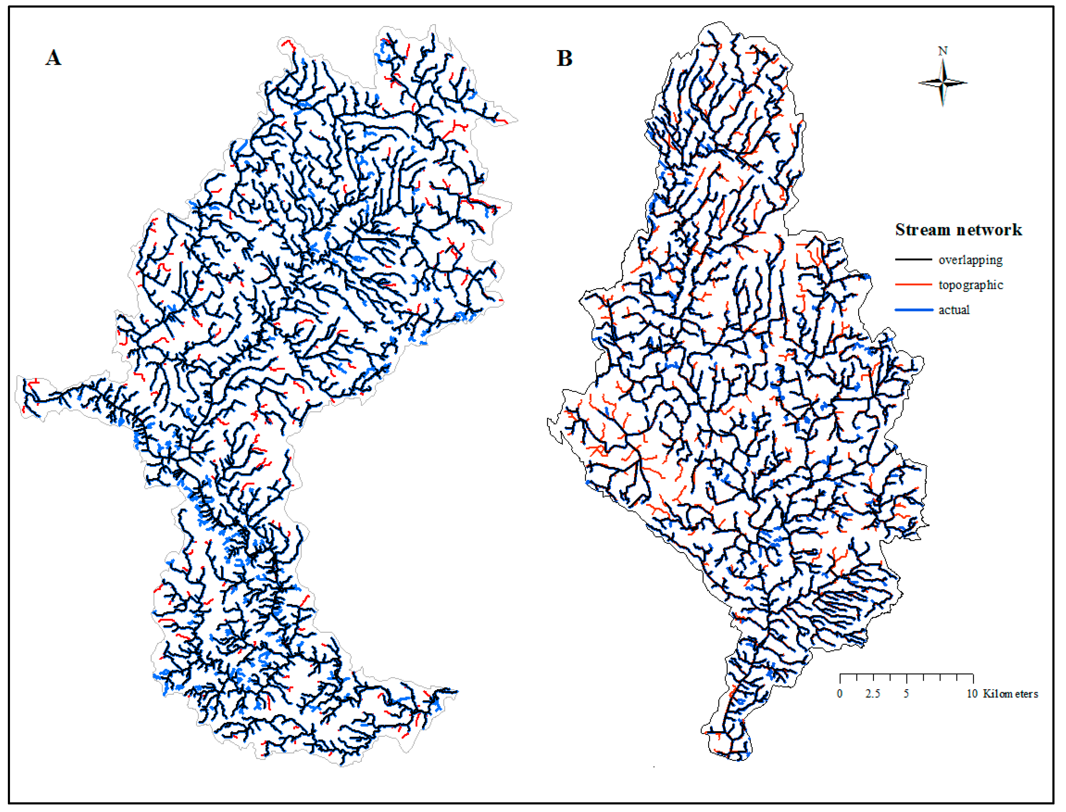
Figure 4.
Stream length of different stream order of the Grand River stream network.
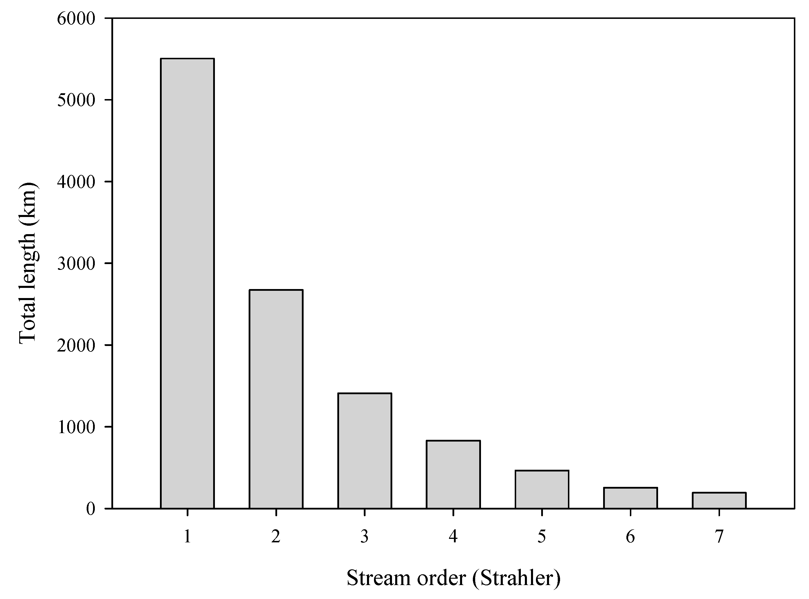
Figure 5.
(a) Simulated stream flow (1980–2010) predicted by SWAT model using DEMs of varying resolutions, (b) comparison of average monthly simulated stream flow (over period 1980–2010) predicted by SWAT model using DEMs of varying resolutions, (c) simulated total suspended solids (1980–2010) predicted by SWAT model using DEMs of varying resolutions, (d) comparison of average monthly total suspended solids (over period 1980–2010) predicted by SWAT model using DEMs of varying resolutions.


Table 1.
Total km of the predicted channels in stream networks derived from DEM models that overlap or lie within varying distances of the existing channels in the Grand River Basin.
Table 1.
Total km of the predicted channels in stream networks derived from DEM models that overlap or lie within varying distances of the existing channels in the Grand River Basin.
| Total Overlap in km (and % Total Channel Length) | |||||||
|---|---|---|---|---|---|---|---|
| DEM Model | 0 m | 2.5 m | 5 m | 10 m | 17 m | 20 m | 40 m |
| 10 m DEM | 8102 (88.2%) | 8209 (89.4%) | 8325 (90.7%) | 8551 (93.1%) | 8727 (95.0%) | 8756 (95.4%) | 8795 (95.8%) |
| 25 m DEM | 7817.6 (87.3%) | 7911 (88.3%) | 8002 (89.3%) | 8174 (91.2%) | – | 8381 (93.6%) | 8512 (95.0%) |
Table 2.
Performance of stream network models derived from 10 m and 25 m DEMs in predicting locations of first and second order channels.
Table 2.
Performance of stream network models derived from 10 m and 25 m DEMs in predicting locations of first and second order channels.
| Stream Characteristics | DEM Resolution | |
|---|---|---|
| 10 m | 25 m | |
| Total length of non-overlapping (within 10 m) first order channels (model predicted versus actual) | 515 m | 598 m |
| % of non-overlapping (within 10 m) channels that are first order (model predicted versus actual) | 81.6% | 76% |
| Number of predicted first order stream segments that do not overlap actual first order channels | 2151 | 3078 |
| Sinuosity of actual first order channels not predicted by DEM | 1.06 | 1.05 |
| Total length of non-overlapping (within 10 m) second order channels (model predicted versus actual) | 101 m | 132 m |
| % of non-overlapping (within 10 m) channels that are second order (model predicted versus actual) | 16.1% | 16.8% |
| Number of predicted second order stream segments that do not overlap actual first order channels | 485 | 877 |
| Sinuosity of actual second order channels not predicted by DEM | 1.06 | 1.04 |
Table 3.
Analysis of stream network and land use in major sub-basins in the Grand River basin.
| Sub-Basin | Area (km2) | Strahler Stream Order (Main Channel) | Sinuosity all Actual Channels | Sinuosity all Predicted Channels (10 m DEM) | Sinuosity Actual First Order Channels | Sinuosity Predicted First Order Channels (10 m DEM) | % Agri. | % Forest/Wetland | % Network Length That is First Order (actual) | Total Predicted Channel Length-10 m DEM (km) | Total Predicted Length First Order Channels-10 m DEM (km) | % Network Length That is First Order (Predicted) |
|---|---|---|---|---|---|---|---|---|---|---|---|---|
| Conestogo River | 819.9 | 6 | 1.13 | 1.12 | 1.13 | 1.11 | 78.0 | 9.2 | 50.0 | 1078.2 | 505.8 | 46.9 |
| Fairchild Creek | 400.7 | 5 | 1.17 | 1.14 | 1.14 | 1.11 | 63.4 | 21.3 | 46.2 | 620.8 | 278.8 | 44.9 |
| Lower Grand | 355.9 | 7 | 1.14 | 1.11 | 1.13 | 1.1 | 62.4 | 22.0 | 48.9 | 482.6 | 233.6 | 48.4 |
| Lower Middle Grand | 475.6 | 6 | 1.17 | 1.15 | 1.13 | 1.12 | 66.0 | 14.7 | 48.6 | 743.3 | 333.9 | 44.9 |
| McKenzie Creek | 368.2 | 5 | 1.21 | 1.13 | 1.15 | 1.10 | 58.8 | 30.5 | 47.8 | 515.3 | 237.5 | 46.1 |
| Middle Grand | 604.6 | 7 | 1.15 | 1.11 | 1.15 | 1.11 | 43.4 | 19.1 | 44.5 | 788.8 | 363.1 | 46.0 |
| Nith River | 1128.0 | 6 | 1.16 | 1.10 | 1.14 | 1.10 | 76.3 | 11.7 | 49.1 | 1487.0 | 682.8 | 45.9 |
| Speed River | 780.8 | 6 | 1.15 | 1.09 | 1.15 | 1.09 | 56.8 | 24.6 | 49.7 | 1031.8 | 508.5 | 49.3 |
| Upper Grand | 791.2 | 6 | 1.13 | 1.10 | 1.13 | 1.10 | 69.9 | 18.9 | 48.0 | 992.9 | 478.8 | 48.2 |
| Upper Middle Grand | 639.8 | 6 | 1.15 | 1.09 | 1.14 | 1.09 | 77.7 | 9.6 | 47.8 | 838.2 | 386.7 | 46.1 |
| Whitemans Creek | 403.9 | 6 | 1.18 | 1.11 | 1.16 | 1.10 | 70.0 | 16.5 | 48.2 | 555.4 | 253.6 | 45.7 |
| Summary | 6768.8 | 7 | 1.16 | 1.11 | 1.14 | 1.10 | 69.7 | 18.0 | 48.1 | 9134.3 | 4263.1 | 46.7 |
Table 4.
Comparison of SWAT models constructed using different DEM resolutions, compared against a SWAT model constructed using a ground-truthed stream network and 10 m resolution.
Table 4.
Comparison of SWAT models constructed using different DEM resolutions, compared against a SWAT model constructed using a ground-truthed stream network and 10 m resolution.
| Hydrology | DEM Resolution | |||
|---|---|---|---|---|
| 10 m with Actual Stream Network | 10 m | 25 m | 200 m | |
| Watershed area | 6782 | 6909 | 6443 | 6358 |
| Sub-basins | 787 | 771 | 742 | 722 |
| HRUs | 7219 | 7357 | 7218 | 4364 |
| Streamflow/precipitation | 0.5 | 0.5 | 0.5 | 0.5 |
| Baseflow/Total flow | 0.34 | 0.33 | 0.34 | 0.33 |
| Surface runoff/Total flow | 0.66 | 0.67 | 0.66 | 0.67 |
| Percolation/precipitation | 0.19 | 0.19 | 0.19 | 0.19 |
| Deep recharge/precipitation | 0.01 | 0.01 | 0.01 | 0.01 |
| ET/precipitation | 0.47 | 0.47 | 0.47 | 0.47 |
| Average stream discharge (m3 s−1) | 126.3 | 126.7 | 121.5 | 119.9 |
| Average sediment discharge (TSS) (mgL−1) | 27.9 | 29.2 | 28.3 | 22.5 |
© 2019 by the authors. Licensee MDPI, Basel, Switzerland. This article is an open access article distributed under the terms and conditions of the Creative Commons Attribution (CC BY) license (http://creativecommons.org/licenses/by/4.0/).
Share and Cite
MDPI and ACS Style
Hanief, A.; Laursen, A.E. Modeling the Natural Drainage Network of the Grand River in Southern Ontario: Agriculture May Increase Total Channel Length of Low-Order Streams. Geosciences 2019, 9, 46. https://doi.org/10.3390/geosciences9010046
AMA Style
Hanief A, Laursen AE. Modeling the Natural Drainage Network of the Grand River in Southern Ontario: Agriculture May Increase Total Channel Length of Low-Order Streams. Geosciences. 2019; 9(1):46. https://doi.org/10.3390/geosciences9010046
Chicago/Turabian StyleHanief, Aslam, and Andrew E. Laursen. 2019. "Modeling the Natural Drainage Network of the Grand River in Southern Ontario: Agriculture May Increase Total Channel Length of Low-Order Streams" Geosciences 9, no. 1: 46. https://doi.org/10.3390/geosciences9010046
Note that from the first issue of 2016, this journal uses article numbers instead of page numbers. See further details here.