Prospecting Glacial Ages and Paleoclimatic Reconstructions Northeastward of Nevado Coropuna (16° S, 73° W, 6377 m), Arid Tropical Andes

Abstract

This work investigates the timing, paleoclimatic framework and inter-hemispheric teleconnections inferred from the glaciers last maximum extension and the deglaciation onset in the Arid Tropical Andes. A study area was selected to the northeastward of the Nevado Coropuna, the volcano currently covered by the largest tropical glacier on Earth. The current glacier extent, the moraines deposited in the past and paleoglaciers at their maximum extension have been mapped. The present and past Equilibrium Line Altitudes (ELA and paleoELA) have been reconstructed and the chlorine-36 ages have been calculated, for preliminary absolute dating of glacial and volcanic processes. The paleoELA depression, the thermometers installed in the study area and the accumulation data previously published allowed development of paleotemperature and paleoprecipitation models. The Coropuna glaciers were in maximum extension (or glacial standstill) ~20–12 ka ago (and maybe earlier). This last maximum extension was contemporary to the Heinrich 2–1 and Younger Dryas events and the Tauca and Coipasa paleolake transgressions on Bolivian Altiplano. The maximum paleoELA depression (991 m) shows a colder (−6.4 °C) and moister climate with precipitation ×1.2–×2.8 higher than the present. The deglaciation onset in the Arid Tropical Andes was 15–11 ka ago, earlier in the most southern, arid, and low mountains and later in the northernmost, less arid, and higher mountains.

1. Introduction

At different time scales, from a few decades to tens of thousands of years, tropical glaciers are highly sensitive indicators of global climate change [1]. This climatic sensitivity can be measured by estimating how the glacier Equilibrium Line Altitude (ELA; meters above sea level, hereafter m) varies with climate. The ELA reconstruction can be done using different mathematical equations, which relate cooling (°C), snow accumulation (mm) and topography (m), in its broadest meaning. The ELA sensitivity to changes in temperature and precipitation is strongly tied to the dominant ablation process, which in turn is determined by the pattern in accumulation [2,3]. Therefore, where precipitation is high, the ablation at the ELA is dominated by melting, and the ELA is more sensitive to changes in temperature. Conversely, in areas with little precipitation, the ablation is dominated by sublimation, and the ELA is more sensitive to precipitation than ablation. Following that criterion based on the ELA response to climate changes, two regions can be differentiated in the Central Andes [4,5]: northern and southern outer tropics (humid Central Andes), where the ELA is more sensitive to changes in temperature, and dry outer tropics (Arid Tropical Andes), where the ELA is more sensitive to changes in precipitation.

Nowadays, precipitation in the Central Andes seems to be linked to boreal cooling because most of the annual precipitation takes place during the Northern Hemisphere winter. We cannot rule out that boreal tropospheric synoptic circulation triggers a change on the south of the Intertropical Convergence Zone (ITCZ), nor that this teleconnection has persisted over the past hundreds to thousands of years. These are merely hypotheses derived from the chronological correlations between the absolute dating of a broad geomorphological and sedimentary (marine and continental) evidence. However, these correlations seem to indicate the existence of interhemispheric connections between related climatic phases:

(a)

Boreal cooling periods, events such as Younger Dryas (YD) and Heinrich (H1... Hn), caused by the Atlantic Meridional Overturning Circulation (AMOC) shutdowns, blocking the inter-hemispheric energy exchange, as a consequence of the marine desalination due to the discharge of icebergs and or freshwater in the North Atlantic.

(b)

Greater moister phases than the present in the humid and arid Central Andes.

Chronological correlation between boreal cooling and Central Andes humidity has been detected in several ways (Figure 1):

-

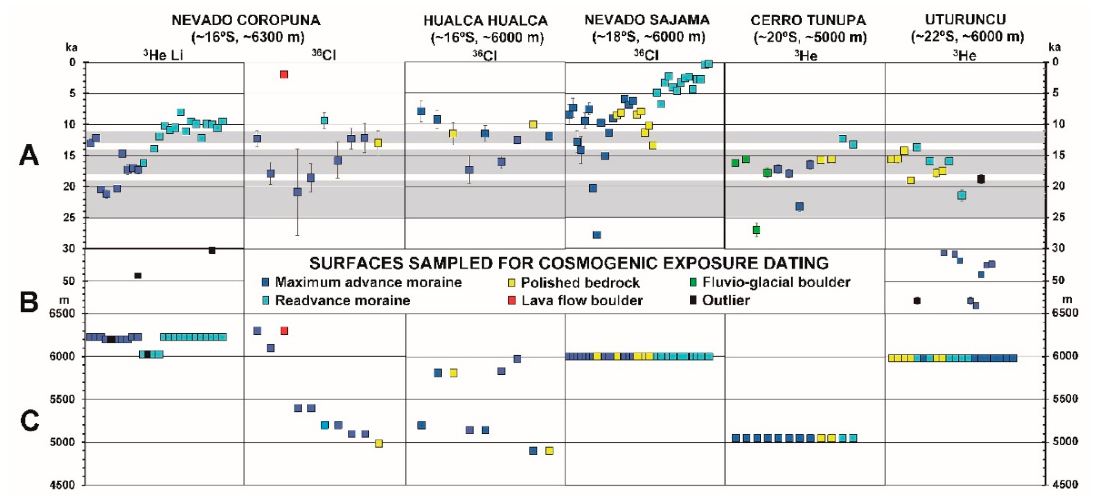
On the one hand, the chronology of moraines shows glacial advances contemporary to cold boreal events, both in glaciers of the eastern tropical Central Andes, which are more sensitive to temperature (e.g., Quelccaya ice cap [6]), and in glaciers of the tropical western Central Andes, which are more sensitive to precipitation (e.g., Ampato-Sabancaya-Hualca Hualca [7]), Cerro Tunupa [8] or Uturuncu volcano [9].

-

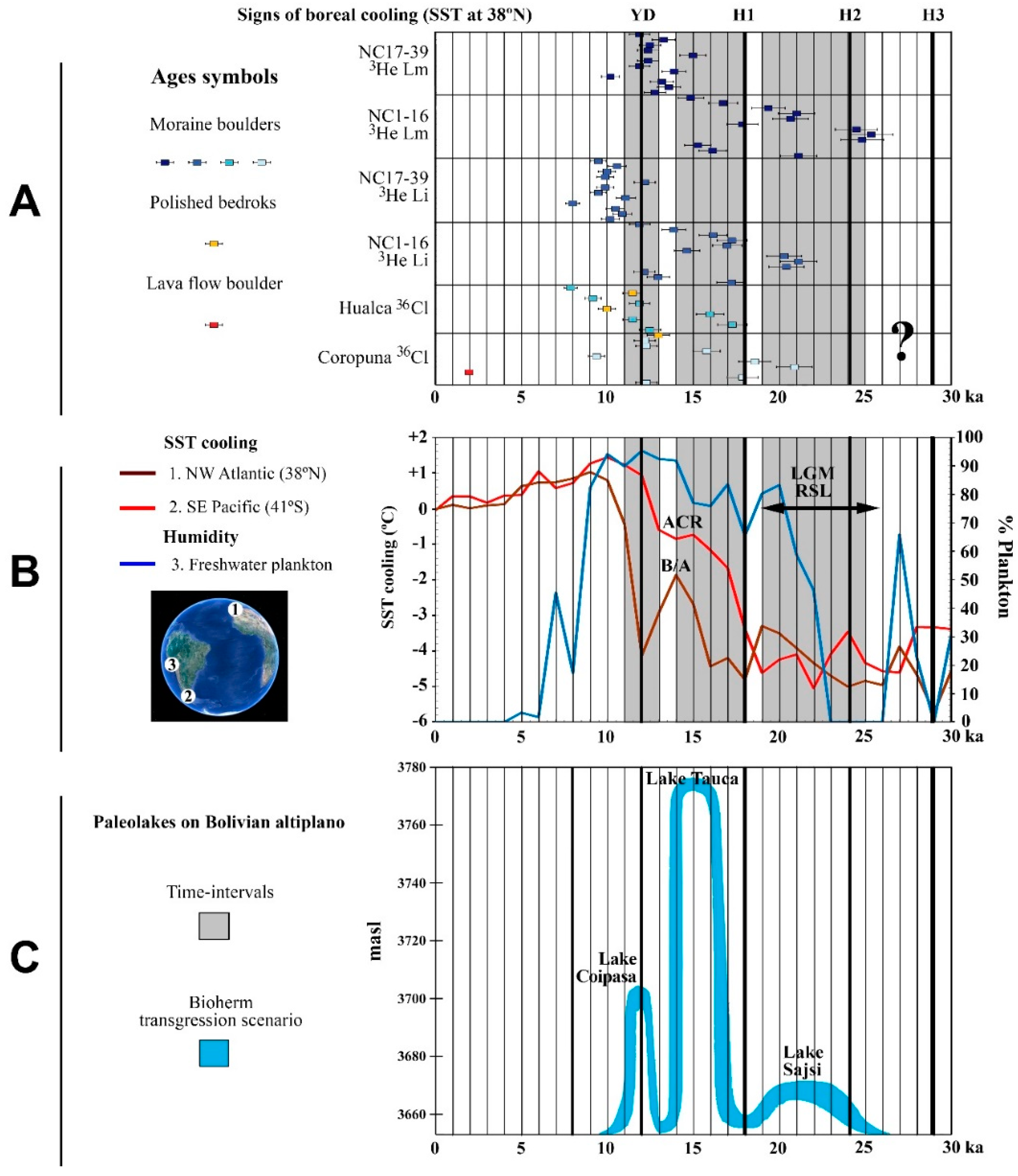
On the other hand, the cold boreal phases have also been chronologically correlated with paleolake transgressions in the Bolivian Altiplano. Blard et al. [10] linked the last big transgressions, Sajsi (~25–19 ka), Tauca (~18–14 ka), and Coipasa (~13–11 ka), to the Younger Dryas (YD) and Heinrich 1 (H1) events. Placzek et al. [11] identified 10 transgressions over the last ~130 ka, contemporary to colder temperatures and iceberg discharges in the North Atlantic. Therefore, the boreal cooling/Andean-moisture-increase teleconnection may have occurred many times throughout the last glacial cycle and even in previous Pleistocene glacial cycles. The ITCZ southward shift have been detected in scales of hundreds [12] to tens of thousands of years [13]. There are many examples: speleothems [14,15], ice cores [16], or marine sediments [17,18].

Numerical models also reveal the climatic link between both hemispheres [19]. The simulations show the ITCZ southward deflection when the North Atlantic is cooled [20,21,22,23] and more recent studies suggest that there is a global atmospheric-teleconnection, among extratropical cooling and tropical humidity through inter-hemispheric thermal contrast [24].

The influence of boreal cooling on Andean glacial advances, by increasing the tropical atmospheric humidity, is captured in the chronological correlations between absolute dating of the Northern Hemisphere paleoclimatic proxies. The most common dating methods in the second half of the 20th century (e.g., ¹⁴C) are well compiled in Clapperton [25]. In the 21st century, most glacial ages are obtained from surface exposure dating [26,27]. Since the pioneering work of [28,29]), many glacial cosmogenic ages have been published whose correlation has been affected by the diversity of the techniques used: distinct isotopes analyzed (¹⁰Be, ³⁶Cl and ³He); differences in chemical sample preparation protocols; accelerator mass spectrometry type (e.g., PRIME or ASTER) and tools used to calculate absolute ages, such as CHLOE [30], CRONUS [31,32,33], CREP [34] or others [35,36]. Previous works [29,37,38,39,40,41] have also pointed out the lack of production rates at low latitude/high altitude sites. Although new production rates are now available for the Central Andes (e.g., [42,43,44]), their publication is recent, and many cosmogenic ages have not yet been recalculated. Shakun et al. and Bromley et al. [45,46] have recalculated ¹⁰Be ages from the Central Andes previously published using the latest version of CRONUS [32] and the new production rates from the Huancane site [44].

Nevertheless, there are no ¹⁰Be glacial ages from the Arid Tropical Andes (~16–22° S) and only ³He glacial ages have been reported from the Coropuna volcanic complex [37,38]; Cerro Tunupa [8] and the Uturuncu volcano [9]. Additionally, there are also some ³⁶Cl glacial ages from the Ampato-Sabancaya-Hualca Hualca volcanic complex and the Patapampa Altiplano [7], which are the only ages related to glacial events in the Arid Tropical Andes recalculated with the new production rates from the Huancane site [44].

A comparison between the results from Coropuna and Hualca Hualca (~16° S), indicates that the available chronologies are, apparently, contradictory:

(a)

Taken together, there are ³⁶Cl ages from moraine boulders [7] showing glaciers in maximum extension ~19–14 ka ago, northward and eastward of the Hualca Hualca volcano. Furthermore, there are ³⁶Cl ages from polished bedrocks, which mark the beginning of the deglaciation, between ~13–11 ka ago in Patapampa Altiplano sites (4950 m) isolated from the surrounding summits, and between ~14–9 ka ago in the lower Pujro Huayjo valley, where glaciers descend from the peaks (>5800 m).

(b)

Nonetheless, the ³He chronology suggests an earlier deglaciation at northeastern Coropuna, in valleys whose summits are >6000 m in altitude. There are moraine boulder ages showing glaciers in maximum extension ~26–15 ka ago [38] and shorter and higher glacial advances in the same valleys ~14–10 ka ago [47].

Moreover, the paleoclimatic reconstructions over the last glacial maximum in the Arid Tropical Andes are not homogenous either. The Coropuna ELA depression shows a ~5 °C cooling regarding the current climate [37,47], if no changes in paleoprecipitation (Δ = 0%) are taken into account. Conversely, another work on Tunupa (~20° S, Figure 1) during the Tauca highstand (~17–15 ka), found somewhat higher cooling (~6.5 °C) and higher precipitation (between ×1.6 and ×3.0) than in the present [8].

The aim of this work is to enhance the knowledge of glacier evolution and the onset of deglaciation in the Arid Tropical Andes, providing new glacial ages, paleotemperature and paleoprecipitation reconstructions, and paleoclimate interpretations.

2. Study Area

2.1. Volcanic Settings

The Nevado Coropuna (16° S, 73° W, 6377 m) is located ~140 km northwest of Arequipa city, ~110 km away from the Pacific Ocean. It is a mountain complex built up by several volcanoes which have grown just on the edge of the narrow ramp that connects the Altiplano with the Pacific coast (Figure 1). The stratovolcano summits reach >6000 m in altitude and they are the watershed limit splitting two deep valleys draining to the ocean: the Arma river valley (western), an Ocoña river tributary, and the Valle de los Volcanes (20 km eastward of Coropuna), flowing into the Colca Valley (tributary of the Majes river). Thick layers of ignimbrites, outcropping westward of the current mountains, suggest that the oldest Coropuna volcanic activity dates back to the Miocene [48]. Through the Pleistocene-Holocene, less explosive volcanic eruptions (dacitic-andesitics) have built the current stratovolcanoes (>6000 m) [49,50]. Almost all Coropuna lava flows are completely glaciated or cut by glacial valleys. However, there are also three lava flows (west, northeast, and southeast of the summit area; Figure 1), only eroded by the latest glacial advances, near the summits. Therefore, it is possible that they are Holocene lavas [51]. However, absolute dating is still not available.

2.2. Climatic Settings

The coast of southern Peru and northern Chile is the most arid region on Earth (annual precipitation <20 mm) as a result of three main causes [52,53,54]: (1) The Andes represent a major topographic barrier to atmospheric circulation in South America; (2) A temperature inversion layer over the Pacific Ocean (700–1000 m) due to the Humboldt cold-water current and (3) Large-scale tropospheric subsidence.

Hence, advections of moist air masses from the Pacific are unlikely and most of the precipitation on the Coropuna glaciers (always snow, because of the high altitude), comes from the Amazon basin, in relation to the South American Summer Monsoon (SASM). As a consequence of the causes mentioned above, one of the main characteristics of the climate is the increase in aridity, southward and westward of the Central Andes [25].

The SASM controls the seasonal precipitation cycle in tropical South America [55,56,57,58], involving several components: the South Atlantic Convergence Zone (SACZ); the convection over the Amazon basin and the ITCZ southward shift during the boreal winter/austral summer, when most of the annual precipitation occurs southward of the Amazon River (Figure 2). However, pollen within the Coropuna glaciers reveal different air masses fluxes. Herreros et al. [59] drilled an ice core at 6080 m altitude, on the Coropuna northern slope, identifying pollen taxa that currently do not exist in that volcanic complex [60,61]:

-

Quercus and Podocarpus: from the Amazon basin, ~300 km northeastward.

-

Nothofagus: native of Patagonia, >3000 km toward the south.

Herreros et al. [59] also measured the mean accumulation rate from 1964 to 2003 (38 years) with an amount of 0.58 m/year. This value is consistent with the annual mean precipitation (500–700 mm) inferred by interpolated data from weather stations (PISCO V1.0; Figure 3; [59]) for the period 1981–2010. Additionally, they reviewed the 1964–2003 climate data in 15 stations around Coropuna, between 3200 and 4270 m in altitude, and reached two main conclusions:

-

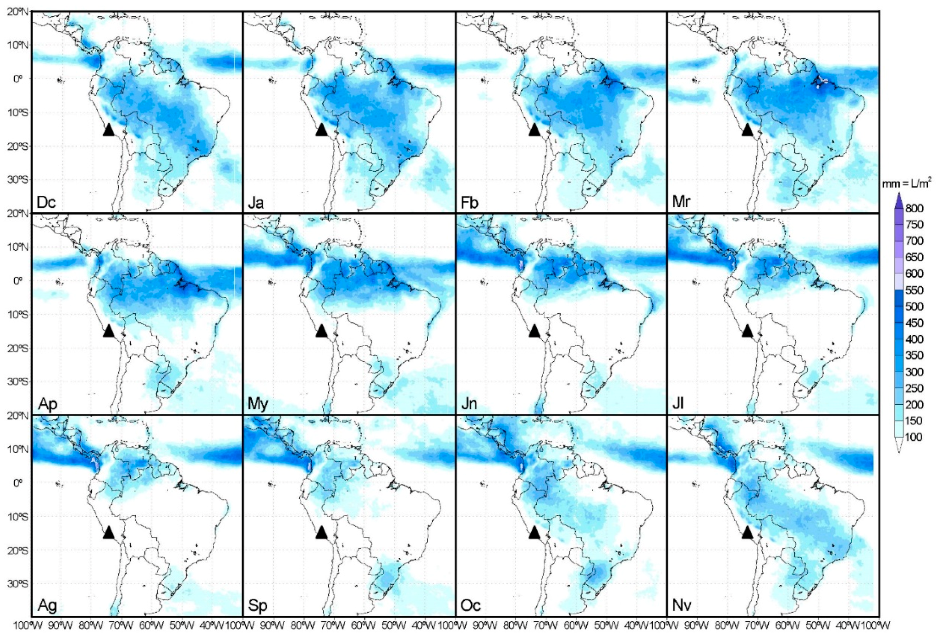
70–90% of the precipitation take place in the austral summer (December-March), coinciding with the ITCZ southward deflection and the winter in the Northern Hemisphere.

-

The precipitation decreased during two El Niño-Southern Oscillation (ENSO) events, in 1982–1983 and 1992, but not in the ENSO 1997–1998.

2.3. Glacial Settings

2.3.1. Glacier Surfaces

The Coropuna summit area is completely covered by many glacier tongues going down the slopes in all directions. In 2010 it was the largest mass of tropical ice on Earth (~46 km²; Figure 1), ~2 km² bigger than the Quelccaya ice cap (14° S, 71° W, 5670 m; ~44 km² [62]). Úbeda et al. [51] mapped the Coropuna glaciers using the ASTER 21/11/2007 satellite image and two orthophotos generated by rectifying the aerial photographs of the only available flights: 21 October 1986 (Servicio Aerofotográfico Nacional, SAN, Lima, Peru) and 15 July 1955 (Instituto Geográfico Nacional, IGN, Lima, Peru). The 1955 aerial photographs show the Coropuna slopes widely covered by snow, even downstream the glacier snouts. However, Úbeda [51] used fieldwork photographs, the ASTER satellite image of 2007 (snow-free) and the orthophoto of 1986 (light snow covering) to accurately delimit the glaciers, in the orthophoto of 1955. This way, he mapped the glaciers and measured their surfaces finding the following results: 56.1 km² (1955), 54.1 km² (1986) and 46.6 km² (2007). These data show a clear acceleration in the deglaciation, at 1986–2007 (7.5 km², 13.9% in 31 years: 0.4 km²/year, 0.7%/year) compared to 1955–1986, when it was 2.0 km², 3.6% in 21 years: 0.1 km²/year, 0.1%. Previously, Ames et al. [63] utilized 1955 aerial photographs but they did not differentiate the slopes covered only by snow, and overestimated the glaciers surface, assuming it was 82.6 km². They were also wrong about the date, thinking that the aerial photos were taken in 1962, like most other flights available in Peru. Both incorrect data (surface and date) have been used in many subsequent works about the Coropuna (e.g., Racoviteanu et al. [64]), who due to the original mistake, calculated wrong values. Kochtitzky et al. [65] have made the most recent and exhaustive work (259 Landsat images 1980–2014), obtaining results and conclusions very similar to Úbeda [51]. Moreover, Kochtitzky et al. [65] have also pointed out previous works mistakes, which interpreted snow as glaciers. Furthermore, they detected lower deglaciation rates and made the most recent measurement of the glacier surface (~44.1 ± 3.9 km² in 2014). The uncertainty in the measurement is due to the fact that the satellite images automatic reclassification is less precise than the vectorial mapping using orthophotos [51].

2.3.2. Snowlines, ELAs and Glacial Dating

Dornbusch [66] reconstructed the snowline altitudes in 1955, at Nevado Coropuna (altitude = 6377 m, snowline₁₉₅₅ = 5200 m) and two nearby stratovolcanoes, Nevado Sara Sara (altitude = 5505 m, snowline₁₉₅₅ = 5200 m) and Nevado Solimana (altitude = 6093 m, snowline₁₉₅₅ = 5430 m). In addition, he used the Terminus Headwall Altitude Ratio (THAR [67,68]) and Area Altitude Ratio (AAR [69]) methods to reconstruct the paleoELAs from the last maximum glacier extension (4300–5400 m), which show a depression of 800–200 m on the snowline₁₉₅₅.

Bromley et al. [37,38] used the CRONUS online calculator [31] to estimate the ³He ages from 30 moraine boulder surfaces, in the Huayllaura valley (southwestward), the Chico valley (westward) and the Santiago and Mapa Mayo valleys, westward of the study area of this work (Figure 1), naming the last one as Ullullo valley. Bromley et al. [37] defined a lower moraine group (~5000–4900 m), extending to the lower area of the glacial valleys, as CI and a higher moraine group (~5500 m), deposited in the middle part of the Santiago valley, as CII. For each group of moraines they found two age ranges, depending on the scaling model used: Lm [70] or Li [71,72,73]:

-

CI moraines: ~25–15 ka (Lm) and ~21–12 ka (Li), with outlier ages ~47 and ~31 ka (Li) and ~61 and ~37 ka (Lm).

-

CII moraines: ~11–12 ka (Lm) and ~11–8 ka (Li).

Bromley et al. [37] grouped together (as pre-CI) the moraine groups eastward of the Mapa Mayo and Santiago valleys, on the Altiplano and in valleys even lower than that plateau. They deduced that the pre-CI moraines were older than the CI moraines, but they did not verify that hypothesis by absolute dating. In a later work, Bromley et al. [47] reconstructed the current ELAs and the paleoELAs around the Coropuna. On the northern slope they estimated an ELA of 5915 ± 44 m. Different paleoELAs were presented for the CI phase, depending on the calculation method or the THAR ratio used:

-

PaleoELA MELM (Maximum Elevation of Lateral Moraines): 5167 ± 59 m.

-

PaleoELAs THAR: 5116 ± 91 m (THAR = 0.25); 5116 ± 89 m (THAR = 0.28) and 5200 ± 88 m (THAR = 0.30); with 5144 ± 89 m average.

Bromley et al. [47] used the paleoELA depression (~750 m) and the air temperature lapse ratio (ATLR) 7–6 °C/km, supposing that the past precipitation had been similar to the present one, to argue that the paleotemperature of the CI phase was ~5.2–4.5 °C colder than nowadays.

Campos [74] used the ASTER 21/11/2007 image and the 15/07/1955 orthophoto from Úbeda [51] to delimit the glaciers in Coropuna southwest side, and reconstruct the ELAs and paleoELAs by the Area x Altitude Balance Ratio method (AABR [75]), achieving the following results: ELA₂₀₀₇ = 5850 m and ELA₁₉₅₅ = 5779 m. Furthermore, he took the mapped moraines [51] to delimit the last maximum glacier advance. Campos [74] defined this maximum advance as Last Glacial Maximum (LGM) but did not support his hypothesis with absolute dating. He also calculated the paleoELA (4762 m) and its depression (ΔELA = 1088 m) regarding the ELA₂₀₀₇ = 5850 m.

3. Methods

3.1. Exposure Ages

3.1.1. Geomorphological Mapping and Fieldwork

Based on the analysis of Google Earth, vertical aerial photographs and orthophotos (IGN 1955 y SAN 1986) and a RapidEye satellite image (6 November 2010) a geomorphological map was made, encompassing the Coropuna northeast and its surrounding area (Figure 4). The map enabled relative dating of the glacial landforms and selection of the appropriate sampling strategy to achieve absolute dating. Due to budgetary constraints and the complexity of the study area, we chose a prospective approach: instead of sampling moraines in a single valley, different moraines in distinct valleys were sampled, along a west-east transect of the geomorphological map. The purpose was to get a preliminary chronology, to guide the future research. In the main valleys of the mapped area, we collected surface samples from large boulders (>1 m in height) located on the moraines crests (Figure 5). Outside these valleys, we also sampled a polished bedrock (Figure 6), in a site topographically isolated from the surrounding mountains, to limit the deglaciation onset in the Altiplano, eastward of Coropuna. Additionally, to estimate the youngest volcanism chronology, we also sampled a boulder surface on the top of the only lava flow not eroded by glaciers, in the mapped area (Figure 7). Sampling tasks also included shielding and erosion field measurements, to weight the exposure ages final calculation. A total of 10 samples were collected (9 from moraine boulders, 1 from polished bed-rock).

3.1.2. Labwork

All the surfaces sampled were volcanic rocks that did not contain quartz. So, to calculate the exposure ages, the accumulation of ³⁶Cl was measured. This is the same cosmogenic isotope used in Hualca Hualca and surroundings [7,76,77], almost at the same latitude (~16° S) but 80–100 km eastward of Coropuna. The same sample preparation protocol [78,79] for the analysis of ³⁶Cl in whole-rock was applied. The organic material was separated from the samples using a metal barbed brush. Then, each sample was crushed in a roller mill and sieved to recover the sand-sized fraction (1–0.250 mm). The chemical preparation was carried out in the PRIME laboratory (Purdue University). Foremost, the sand fraction size was leached in deionized water and HNO₃, to remove atmospheric Cl. Thereafter, each sample was dissolved in a mixture of HNO₃ and HF acids. In the dissolution process, a spike of isotopically enriched ³⁵Cl was added. The isotope dilution method allowed the ³⁶Cl and total Cl to be measured simultaneously [80]. The ratios ³⁶Cl/Cl and ³⁷Cl/³⁵Cl were measured in the Accelerator Mass Spectrometry (AMS) of PRIME lab. In the Activation Laboratories (Ancaster, ON, Canada), aliquots of the total mass of rock and the target fraction were analyzed using the following methods to determine the abundances of the parent isotopes of Ca, K, Ti and Fe, which produce ³⁶Cl from spallation and muon capture:

(a)

Major elements: by inductively coupled plasma optical emission spectrometry (ICP-OES).

(b)

Trace elements: by inductively coupled plasma mass spectrometry (ICP-MS).

(c)

Boron: by prompt-gamma neutron activation analysis (PGNAA).

The field and analytical data are presented in

Table 1. Field and analytical data for ³⁶Cl exposure ages from northeast of Coropuna and surroundings.

Sample ID		NCNE01	NCNE02	NCNE03	NCNE04	NCNE05	NCNE06	NCNE07	NCNE08	NCNE09	NCSE23
Geomorphological Unit		Moraine Boulder	Moraine Boulder	Lava Flow Boulder	Moraine Boulder	Moraine Boulder	Moraine Boulder	Moraine Boulder	Moraine Boulder	Moraine Boulder	Polished Bedrock
CRONUS ages	(ka)	12.3 ± 1.3	17.9 ± 1.8	2.0 ± 0.4	20.9 ± 6.9	18.6 ± 2.3	9.4 ± 1.3	15.8 ± 2.9	12.3 ± 1.7	12.2 ± 2.4	13.0 ± 2.0
Latitude	(°S)	−15.50	−15.51	−15.51	−15.52	−15.51	−15.51	−15.51	−15.48	−15.48	−15.54
Longitude	(°W)	−72.58	−72.56	−72.55	−72.55	−72.54	−72.53	−72.50	−72.45	−72.43	−72.49
Altitude	(masl)	5060	5013	4901	4915	5052	4929	4914	4384	4080	4914
Erosion rate	mm/ka	0.4	0.3	0.0	0.3	0.0	0.8	0.3	0.8	0.4	0.0
Sample thickness	(cm)	1.50	2.00	3.00	2.50	2.50	2.50	2.00	2.00	4.00	2.50
Bulk density	(g·cm−3)	2.49	2.27	2.18	2.55	2.48	2.76	2.45	2.27	2.53	2.49
Shielding factor	(unitless)	0.99	1.00	0.99	0.99	0.99	1.00	1.00	0.99	0.99	1.00
Effective fast neutron attenuation length	(g·cm−2)	169.56	166.99	170.78	164.45	159.59	170.40	165.70	164.94	170.80	170.40
Na2O	(wt %)	4.51	4.41	4.52	4.33	4.35	4.29	4.17	3.41	3.42	4.31
MgO	(wt %)	1.95	1.98	1.88	2.57	2.64	2.64	2.93	0.72	1.09	2.98
Al2O3	(wt %)	15.80	15.35	16.15	15.84	16.02	16.08	16.05	14.57	15.42	16.47
SiO2	(wt %)	62.62	62.61	61.89	59.22	59.41	60.20	58.20	69.96	66.94	57.80
P2O5	(wt %)	0.48	0.37	0.36	0.45	0.50	0.60	0.65	0.16	0.16	0.51
K2O	(wt %)	2.91	2.88	2.97	2.69	2.73	2.80	2.44	3.59	3.25	2.44
CaO	(wt %)	4.54	4.38	4.36	5.21	5.36	4.88	5.56	2.05	2.74	5.56
TiO2	(wt %)	0.80	0.78	0.93	0.99	1.02	0.99	1.20	0.39	0.43	1.20
MnO	(wt %)	0.07	0.07	0.06	0.08	0.08	0.08	0.09	0.04	0.09	0.07
Fe2O3	(wt %)	4.72	5.00	5.44	6.18	6.27	5.91	7.15	3.34	3.89	6.96
Cl	(ppm)	7.10	6.30	22.10	13.10	11.90	7.10	31.10	16.30	3.20	18.30
B	(ppm)	14.70	8.70	17.50	9.50	4.30	15.90	5.90	8.40	14.30	5.00
Sm	(ppm)	6.00	5.80	5.70	6.80	6.90	6.80	6.80	3.00	3.80	7.00
Gd	(ppm)	3.70	3.60	3.80	4.30	4.50	4.30	4.90	2.20	3.10	5.00
U	(ppm)	1.40	1.40	1.50	1.00	0.80	1.10	0.90	2.90	3.00	0.90
Th	(ppm)	6.80	7.00	8.40	5.40	5.50	5.70	5.00	12.30	11.10	5.30
Cr	(ppm)	20.00	20.00	20.00	60.00	80.00	60.00	50.00	<20	40.00	80.00
Li	(ppm)	0.00	0.00	0.00	0.00	0.00	0.00	0.00	0.00	0.00	0.00
36Cl/Cl ratio de-spiked	(36Cl/1015Cl)	862.90	1259.00	79.30	969.90	776.50	584.90	481.20	453.70	449.60	492.6
36Cl/Cl 1σ uncertainty (de-spiked)	(36Cl/1015Cl)	28.15	46.67	4.79	51.38	16.19	22.90	10.99	10.72	17.70	15.96
Sample mass disolved	(g)	32.32	31.54	30.13	30.57	30.79	30.48	30.08	30.26	30.20	30.22
Mass of 35Cl spike solution	(g)	1.02	1.02	1.04	1.05	1.00	1.02	1.05	0.99	1.05	1.03
Concentration spike solution	(g g−1)	1.00	1.00	1.00	1.00	1.00	1.00	1.00	1.00	1.00	1.00
Analytical stable isotope ratio	(35Cl/35Cl + 37Cl)	6.33 ± 0.31	6.96 ± 0.32	3.58 ± 0.02	4.38 ± 0.49	4.20 ± 0.02	6.00 ± 0.47	3.56 ± 0.03	4.10 ± 0.03	5.09 ± 0.43	3.92 ± 0.03
Analytical 36Cl/Cl ratio	(36Cl/1015Cl)	862.9 ± 28.2	1259.0 ± 46.7	79.3 ± 4.8	969.9 ± 51.4	776.5 ± 16.2	584.9 ± 22.9	481.2 ± 11.0	453.7 ± 10.7	449.6 ± 17.7	492.6 ± 16.0

.

3.2. ELA and PaleoELA Reconstruction

The mapping of paleoglaciers (Figure 7), based on the geomorphological map, led to the ELA and paleoELA reconstruction by the AABR method [75], because where good topographic maps and air photograph coverage are available, this method is more rigorous than any other [81]. The application of the same method for current ELAs and paleoELAs is almost a novelty in the Tropical Andes because, with few exceptions [77,82], previous works in Coropuna [47] and other mountains [83] used different procedures for the present and the past. In this work, in addition to the ELAs, the paleoELAs corresponding to two consecutive stages of a hypothetical maximum glacial extension were reconstructed. The extension of these stages (not their interpretation) corresponds to the two oldest phases (CI and pre-CI) previously defined in the same study area [37]:

(a)

PaleoELA₁ (CI phase): maximum glacier advance within the valleys connected to the highest Coropuna peaks (>5200 m).

(b)

PaleoELA₂ (pre-CI phase): maximum glacier advance, covering the whole of the Altiplano and reaching even lower valleys towards the northeast and east of the Coropuna.

The results allowed to elaborate the paleoELA spatial models, selecting the contour line segments, with equivalent altitude, included within the paleoglacial limits. This way, the accumulation zones were identified in the two maximum glacial extension phases corresponding to paleoELA₁ and paleoELA₂.

3.3. Paleoclimate Reconstructions

3.3.1. Paleoclimate Cooling

The temperature depression was deduced by solving a product widely used in previous works (e.g., Sutherland et al. and Porter et al. [84,85]):

$$∆\mathrm{T}=\mathrm{ATLR}\times \Delta \mathrm{ELA}$$

(1)

where: ΔT is the paleoclimate cooling recorded by paleoglacier extension (°C); ATLR the Air Temperature Lapse Rate (°C/m) and ΔELA the paleoELA depression (m). To obtain the ATLR value necessary to solve Equation (1), air temperature data were used from the records measured throughout the period from 1 January 2010 to 31 December 2010 by thermometers installed in the study area (CRYOPERU project; https://cryoperu.pe/). However, one year is a relatively small interval of time to obtain a representative lapse rate. Moreover, paleolake transgressions on the Bolivian Altiplano (e.g., Blard et al. [10] and Clayton et al. [86]) show that the Arid Tropical Andes paleoclimate was moister than in the present, which would have implied a smaller ATLR. Therefore, to solve Equation (1), the temperature lapse rate from the International Standard Atmosphere (ATLR_EARTH = 6.5 °C/km), suitable for the tropics [1], and the local value (ATLR2010 = 7.0 °C/km) were applied.

3.3.2. Paleoprecipitation

Equation (1) assumes that in the past the precipitation was similar to the current one. However, for exploratory purposes, the precipitation reconstruction was carried out using an equation [87] slightly adapted for this work as follows:

$$\mathrm{ELA} = \mathrm{Fc} + 1.01\mathrm{F} \mathrm{z} – 0.51\mathrm{P}$$

(2)

where: Fc is a geographical correction factor defined in this work (537 in Green et al. [87]), being the first variable to be solved, by testing Equation (2) with the values found for the other parameters:

-

ELA (m): Equilibrium Line Altitude by the AABR method in the year analyzed (ELA₂₀₁₀).

-

Fz (m): Annual average freezing-altitude.

-

P (mm): Total annual precipitation at the ELA.

However, Equation (2) represents a statistical average from tropical glaciers and should be carefully evaluated when is applied in each study site [88]. Besides, the Coropuna glaciers are more sensitive to precipitation than to temperature [4,5]. For both reasons, we tested Equation (2) using the value of Fc = 635, which allowed us to obtain the ELA₂₀₁₀, using the following values for the other variables:

-

Fz (m): annual average freezing-altitude (Fz₂₀₁₀ = 5589 m), calculated from the 1 January 2010–31 December 2010 data recorded by CRYOPERU thermometers in the CORNE11 (4886 m) and CORNE41 (5822 m) stations. In this calculation, the ATLR_EARTH = 6.5 °C/km gradient was applied.

-

P (mm): Extrapolated precipitation for the ELA AABR level, obtained by extrapolating the average annual accumulation (580 mm) in the ice core at 6080 m altitude [59] with the Precipitation Lapse Rate PLR = 0.1 mm/m, as Klein et al. [89].

Precipitation was deduced by using the following equation, derived from the Equation (2), once adapted with the data of the reference year (ELA₂₀₁₀ and Fz₂₀₁₀).

$$\mathrm{P} = \left(\mathrm{Fc} + 1.01\mathrm{Fz} –\mathrm{paleoELA}\right)$$

(3)

where:

-

P (mm): Paleoprecipitation in the time of maximum paleoELA depression (equivalent to maximum glacier extension).

-

Fc = 635 (as explained previously).

-

Fz (m) is the annual average freezing-altitude estimated for the past, which was obtained by subtracting the ΔT (°C), deducted in Equation (1), to the air temperature annual mean (°C) in the CORNE4 station.

-

PaleoELA (m) is the ELA AABR in the maximum glacier extension (PaleoELA₂ in the pre-CI phase).

To solve Equation (3), 2 values of ATLR were used: one deduced from CRYOPERU data and another taken to be the value suitable for the tropics (ATLR = 6.5 °C/km [4]).

4. Results

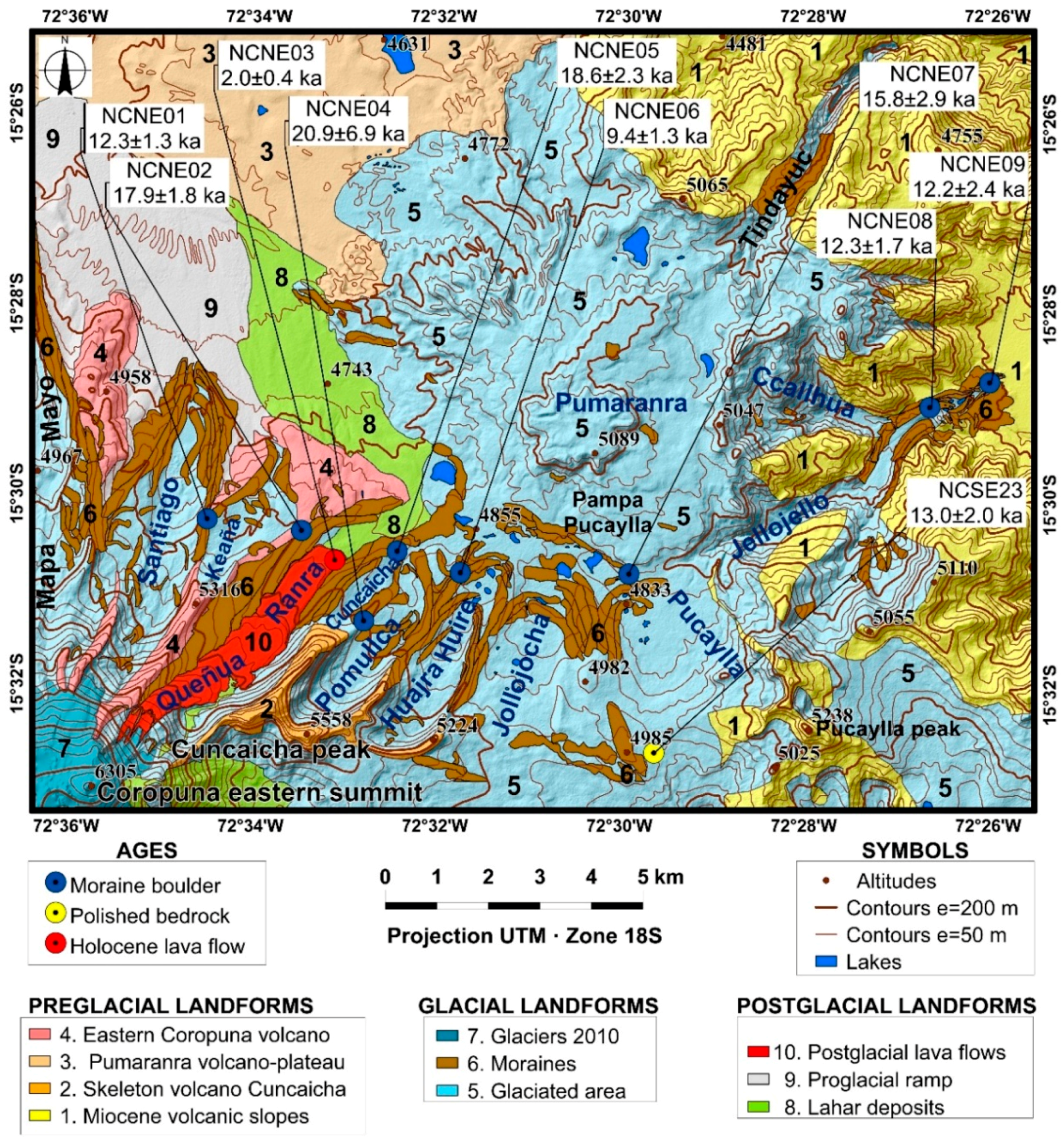
4.1. Geomorphological Map

Preglacial, glacial and postglacial volcanic landforms were mapped (Figure 4; numbers 1–10).

4.1.1. Preglacial Landforms

The following preglacial landforms, previous to the maximum glacial extension, were identified:

(1)

Miocene volcanic slopes (<5100 m): pre-Quaternary hillsides [90] non-eroded by glaciers connecting topographically the South American Altiplano surrounding the current Coropuna and the bottom of the deepest valleys located at the east and the south of the mapped area.

(2)

Volcano-skeleton Cuncaicha (5558 m): A hydrothermalized volcanic structure, strongly eroded by glaciers, adjacent to Coropuna.

(3)

Pumaranra volcano-plateau (5089 m): small flattened summit, only ~100 m higher than the Altiplano, and lava flows scattered around this emission center.

(4)

Eastern Nevado Coropuna (>6000 m): highest and youngest stratovolcanoes, whose summits are currently completely glacier covered.

4.1.2. Glacial Landforms

The current glaciers have been mapped (7), as well as their reconstructed last maximum extension (5) based on large lateral and terminal moraines (6) deposited in the following sites:

-

Northward of the Coropuna eastern summit (6305 m) and the Cuncaicha peak (5558 m): the Mapa Mayo, Santiago, Keaña, Queñua Ranra, Cuncaicha, Pommullca and Huajra Huire valleys.

-

Pampa Pucaylla Altiplano, a little endorheic basin where ice tongues arrived from slightly higher surrounding areas: Cerro Pumaranra (northward); Pucaylla Peak (toward southeast) and the watershed-splitting linking the eastern Cuncaicha Peak foothills and the western flank of Pucaylla Peak.

-

Tindayuc, Callhua and Jellojello Valleys, which channeled the past glacier advances, overflowing the Pampa Pucaylla northeast and east limits and going down towards the Valle de los Volcanes.

Moreover, many smaller moraines (6) are found at increasingly higher altitudes, because after the deglaciation onset, the ice cap shrinking trend has sometimes been interrupted by small glacial pulses.

4.1.3. Postglacial Landforms

Landforms due to volcanic processes, which occurred after the last maximum glacial extent, also have been mapped:

-

Proglacial ramp (9) covered by ash, lapilli, and volcanic bombs.

-

Postglacial lava flow (10) and lahar deposits (8) in the Queñua Ranra valley.

4.2. Geomorphological Analysis and ³⁶Cl Ages

The ³⁶Cl ages from the sampled surfaces are presented below, in the context of their location and geomorphology (Figure 5 and Figure 6, Table 1).

4.2.1. Coropuna Northeast Slope

(a)

Santiago Valley

The valley begins at the eastern Coropuna summit (6305 m) and descends 8 km towards the north, reaching the altiplano at ~4700 m. The upper valley is divided into two gorges converging at ~5100 m. From this site, two large lateral moraines descend to the lower valley delimiting its western and eastern margins. Each of these sets consist of several generations of lateral moraines attached to each other. Sample NCNE01 was collected on a boulder surface located in the eastern set of moraines. It indicates an age of 12.3 ± 1.3 ka for the maximum glacial advance in the Santiago valley. At the bottom of the valley there are ~8–10 generations of smaller moraines, the highest at ~5600–5800 m in altitude, near the current glaciers snouts (Figure 4 and Figure 8).

The upper valley is divided into two gorges converging at ~5100 m. From this site, two large lateral moraines descend to the lower valley delimiting its western and eastern margins. Each of these sets consist of several generations of lateral moraines attached to each other. Sample NCNE01 was collected on a boulder surface located in the eastern set of moraines. It indicates an age of 12.3 ± 1.3 ka for the maximum glacial advance in the Santiago valley. At the bottom of the valley there are ~8–10 generations of smaller moraines, the highest at ~5600–5800 m in altitude, near the current glaciers’ snouts (Figure 4 and Figure 8).

(b)

Keaña Valley

It has been slightly excavated on top of an old lava flow, on the eastern Coropuna volcano (Figure 4). This lava flow has been eroded through by the Santiago and Queñua Ranra glacial valleys headwaters. The Keaña Valley onset is the north face of a 5316 m high hill. Thence, the valley descends towards the northeast for ~2 km, ending in large lateral moraines deposited at ~4850–4800 m. Upslope of these lateral moraines there are 3–4 generations of recessional moraines, in an interval between ~4950 and ~5050 m in altitude.

(c)

Queñua Ranra Valley

Its wide head is at ~5950 m altitude, northeastward of the glaciers that are completely covering the Coropuna eastern summit (6305 m). Thence, the Queñua Ranra descends towards the northeast, confined between multiple and contiguous lateral moraines on each side of the valley. Sample NCNE02 was collected in the eastern side, pointing to an age of 17.9 ± 1.8 ka for one of the possible maximum advances (perhaps glacial standstill) in the Queñua Ranra Valley. This valley ends with a terminal moraine that closes a topographic depression, seasonally filled by a lake, at ~4800 m in altitude and ~10 km far away from the mountain summit. The geomorphological evidence indicates a vulcanian eruption from the Coropuna eastern summit after the valley’s deglaciation. A lava stopper probably obstructed the crater before the eruption. Nowadays the stopper pieces are volcanic bombs scattered in the lower Queñua Ranra Valley (Figure 5). The geomorphological evidence also suggests that the sudden thaw due to the eruption, triggered a lahar which was channeled down the valley. The lahar overflowed the western lateral moraines, spreading out northwestward over the altiplano and reaching ~4650 m minimum altitude, ~14 km away from its source area. Finally, the volcanic eruption emitted a lava flow which partially filled the Queñua Ranra Valley bottom. The lava snout went down to an altitude of ~4900 m and ~6–7 km away from the emission focus, which could have been located right at the summit, below the current glaciers. The NCNE03 sample was collected on a boulder above the lava flow snout. This suggests that eruption occurred 2.0 ± 0.4 ka ago. Further up the valley, there is another lava flow overlaying the sampled lava. The snout of this second lava flow is higher (~5050 m) and closer (~5 km) to the stratovolcano summit than the first one. Nonetheless, no absolute dating has been done to discern whether the two lava flows were emitted at the same time or by diachronic eruptions. The pyroclastic deposits covering the proglacial ramp (Figure 4) were probably also emitted by those same volcanic eruptions. Inside the Queñua Ranra Valley, the lahar and the lava flows partially eroded or covered almost all recessional moraines. However, there are well preserved younger moraines on the upper lava flow (Figure 8). These moraines were deposited after the volcanic eruptions, possibly at the Little Ice Age.

4.2.2. Cuncaicha Peak North Face

(a)

Cuncaicha Valley

It is a small and very narrow valley beginning at the base of the northernmost foothills of the Cuncaicha peak (5558 m), between the Queñua Ranra and Pomullca Valleys. The Cuncaicha Valley follows a southwest-northeast direction, is ~1–2 km in length and ends on the western lateral moraine of the Pomullca Valley.

(b)

Pomullca Valley

The head of the valley is a horseshoe shaped cirque facing the northeast. It has been excavated by the glaciers of the northern slope of the Cuncaicha peak. From the glacial cirque exit, the Pomullca Valley descends towards the northeast and is characterized by the presence of large lateral moraines. Afterward, the glacial valley turns sharply northward and ends at a terminal moraine deposited at ~5050–4850 m in altitude and ~4 km away from the head of the valley, above the Queñua Ranra Valley eastern lateral moraine. The NCNE04 sample was collected in a boulder on the western Pumullca moraine, close to the cirque lip. Its absolute dating suggests a maximum advance (or glaciers standstill) at 20.9 ± 6.9 ka ago. The NCNE05 sample was collected from another boulder on the Pumullca terminal moraine, over the Queñua Ranra eastern lateral moraine. Its dating suggests another maximum advance (or glacial standstill) 18.6 ± 2.3 ka ago. Further up there are 3–4 generations of recessional moraines, between ~4900 and ~5100 m in altitude.

(c)

Huajra Huire Valley

The Cuncaicha peak foothills extend eastward, decreasing progressively down to 5224 m in altitude (Figure 4). The Cuncaicha Peak foothills northern face is the Huajra Huire Valley headwater, which also has a horseshoed shaped cirque facing northeast. Thence, the Huajra Huire Valley goes down ~5 km towards the northeast, up to 4855 m in altitude. There, the valley turns sharply to the southeast and ends ~2 km away, in a terminal moraine closing a topographic depression that is seasonally filled by a lake. The NCNE07 sample was collected on a boulder above the Huajra Huire terminal moraine. Its dating suggests that a maximum glacial advance (or glacial standstill) reached the moraine 15.8 ± 2.9 ka ago. Further up the valley, there are two recessional moraine groups and three small seasonal lakes interspersed between both sets, at ~4900 m in altitude. In the lowest set, the NCNE06 sample was collected. Its age seems to point to an advance (or glacial standstill) in the middle of the Huajra Huire valley, 9.4 ± 1.3 ka ago. Although only one age is limited evidence, it seems to indicate a smaller advance than the maximum extension, which would mean that the deglaciation had already begun. Near the valley head, two generations of smaller moraines were probably deposited by the last minor advances, before the complete summit deglaciation.

4.2.3. Glacier Source Areas that Flowed into the Pampa Pucaylla Altiplano

(a)

Jollojocha Valley

It is a very broad valley, but not as deep as the valleys connected to the Coropuna and Cuncaicha summits. The Jollojocha Valley head is a line dividing two drainage basins, because it is also the Coropuna southeastern headwaters. The Jollojocha valley head consists of two different areas (Figure 4):

-

The western area is the outer face of the Huajra Huire Valley headwater, eastward of the 5224 m peak.

-

The eastern area is ~2 km toward the east, at around 4985 m.

From the double headwater the valley goes down ~2 km northward, ending at Pampa Pucaylla Altiplano. There, 1–3 terminal moraines close a topographic depression, which a lake fills seasonally, at ~4840 m in altitude. Upstream of the terminal moraines there are 2–3 recessional moraines, between which a small depression and a seasonal lake are also interspersed.

(b)

Pucaylla Valley

Two head areas can be distinguished in this overall broad valley:

-

The western area has a lower, reaching 4985 m in altitude in the line dividing the northeastern and southeastern Coropuna drainage basins (Figure 7).

-

The eastern area is higher (~5200 m). It is on the Pucaylla Peak northwest face (5238 m).

From both sites, the Pucaylla Valley goes down ~4 km towards Pampa Pucaylla, where three terminal moraines, at ~4825 m in altitude, have small depressions interspersed (seasonally filled by lakes).

(c)

Pumaranra volcano-plateau

This small plateau shaped volcanic structure is ~12 km northeastward of the Coropuna eastern summit. This plateau shape is due to strong glacial erosion, perhaps over several hundred thousand years. The glaciated area and a few moraines in the Pumarranra surroundings can be identified in aerial photographs and satellite images. This suggests that the Pumaranra was covered by a small ice cap, projecting glacier tongues in all directions:

-

South: the Pumaranra glaciers roved only ~1 km and deposited terminal moraines leaning on the moraines of the Queñua Ranra, Pomullca, Huajra Huire, Jollojocha, and Pucaylla Valleys.

-

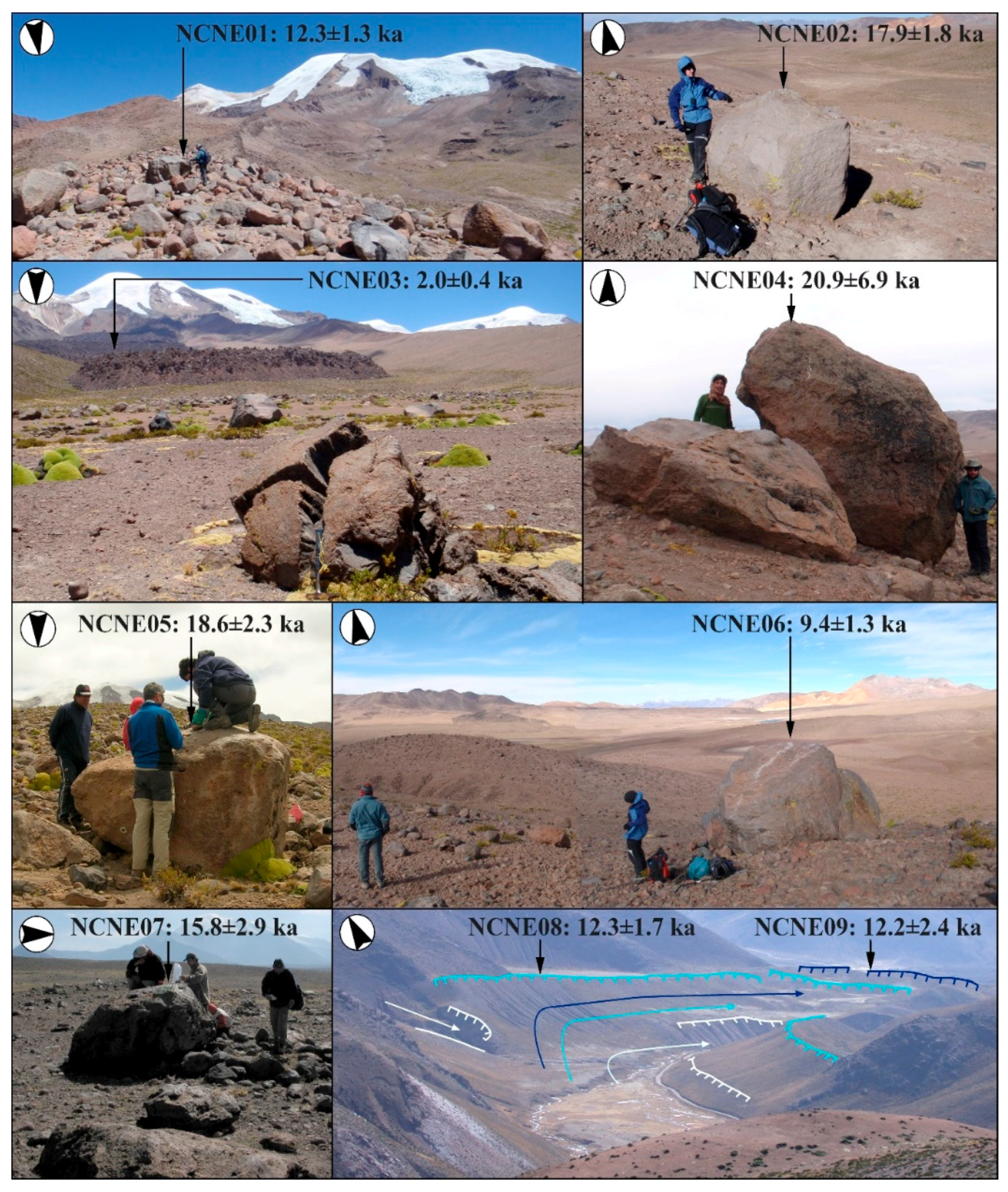
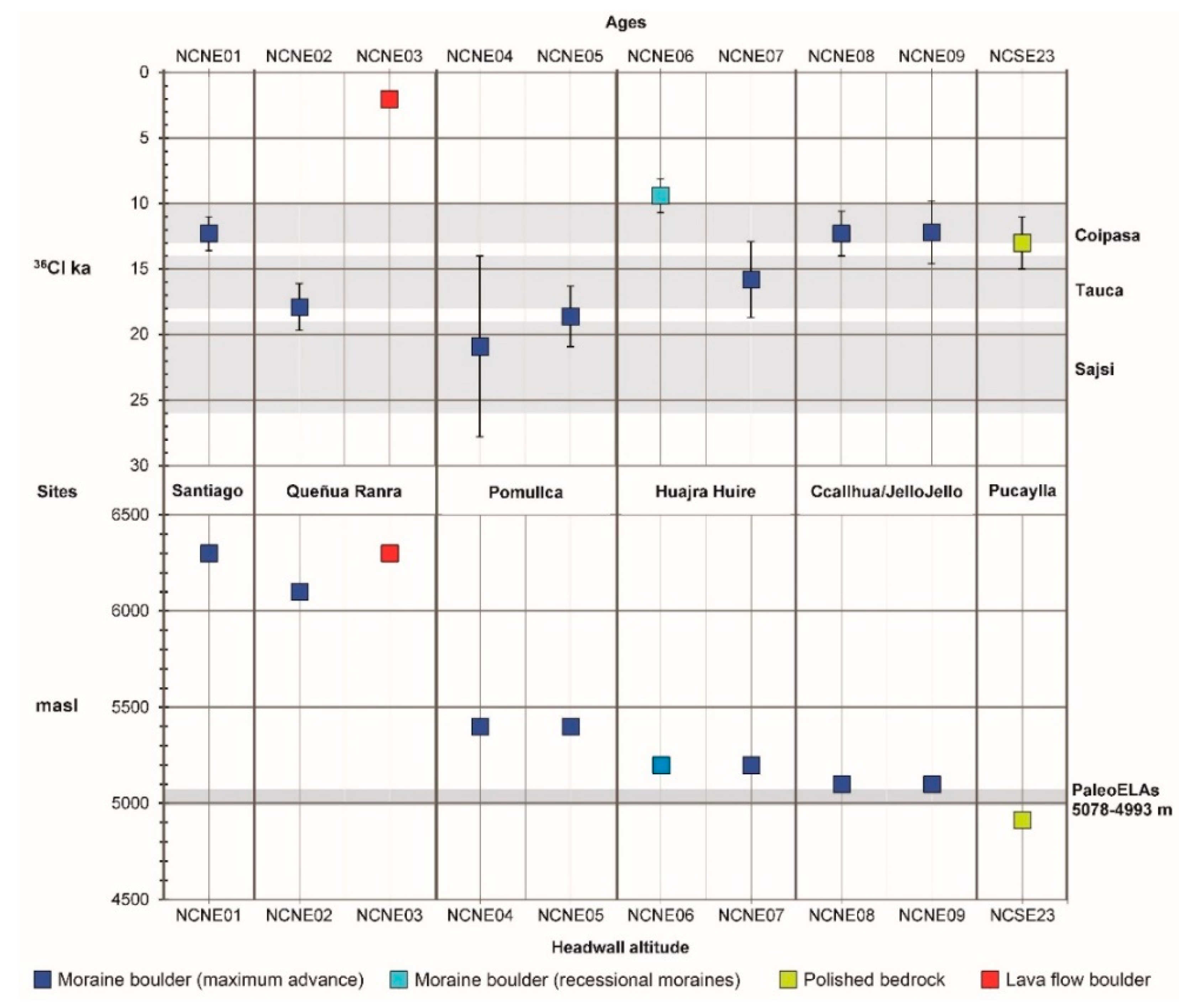
Southeast: the Pumaranra glaciers converged with others descending from the Pucaylla peak north face. This confluence gave rise to a larger glacier, which was channeled within the Jellojello Valley, depositing at least four generations of lateral and terminal moraines, at ~4200 m in altitude, ~3–4 km away from the glaciers confluence, and ~6–8 km from the Puchalla Peak and the Pumaranra volcano-plateau. In the Jellojello Valley moraines, the surfaces of two boulders (samples NCNE08 and NCNE09) were sampled. Their absolute dating suggests, respectively, maximum advances (or glacial standstill) of 12.3 ± 1.7 ka and 12.2 ± 2.4 ka ago.

-

East: the Pumaranra glaciers overflowed the Pampa Pucaylla Altiplano east boundary, a north-south alignment of summits between ~5050 and ~5000 m in altitude. Once over this obstacle, the ice tongues descended through the Ccallhua Valley to where it meets the Jellojello Valley. Here a terminal moraine was embedded by Ccallhua glaciers in the Jellojello Valley lateral moraines (Figure 4), at ~4300 m altitude and ~6 km away from Punmaranra volcano-plateau.

-

Northwest and west: well-defined moraines are not conserved, or are too small to be observed by remote sensing and/or mapped in our work scale. However, the glaciated area can be clearly identified in aerial photographs and satellite images, through changes in the surface appearance due to glacial erosion.

4.2.4. Altiplano Areas Topographically Isolated from the Surrounding Mountains

The glaciers reconstruction (Figure 7), based on the mapped lateral and terminal moraines (Figure 4), suggest that the Pampa Pucaylla Altiplano was completely covered by ice masses fed by the surrounding mountains. The whole area is widely covered by ablation moraines, while polished bedrock outcrops have not been found, which could have allowed the chronological control of the Altiplano deglaciation onset to be determined. It is likely that the flatness and endorheism of Pampa Pucaylla would have allowed the excellent preservation of ablation moraines, impeding the boulder transport outside the area. In contrast, southward of the western Pucaylla Valley head, where the steep slopes of the southeastern Coropuna begin, no ablation moraines are preserved and there are abundant polished bedrocks. The direction of striation indicates that the glaciers that eroded these surfaces came from the southern side of Pucaylla eastern headwater, at 4985 m in altitude. Thence, the glaciers went down to ~3600 m, outside the area drawn on the geomorphological map. On a polished bedrock at 4915 m, near the southern side of Pucaylla eastern headwater (at an elevation of 4885 m) the NCSE23 sample was collected. Its exposure age suggests that the deglaciation of that topographically isolated area from the surrounding mountains began 13.0 ± 2.0 ka ago.

4.3. ELA, PaleoELAs, Climate Cooling and Paleoprecipitation

In 2010, 2 glaciers at the Santiago Valley head and 5 glaciers at Queñua Ranra Valley head were still in existence (Figure 8). They are the only current ice tongues to the northeastward of Coropuna. Following the method proposed by Osmaston [75]: first, the ELAs were tabulated in series with the BR values used for their estimation. Then, the averages and standard deviations of the statistical series were calculated. Finally, the average linked with the smallest standard deviation was selected as the most likely ELA. This is how the ELA was estimated in the Santiago and Queñua Ranra valleys: ELA₂₀₁₀ = 5984 m/BR = 1.0 (

Table 2. ELAs AABR 2010 and Balance Ratio (BR) applied.

Glaciers		BR = 1.0	BR = 1.5	BR = 2.0	BR = 2.5	BR = 3.0
Santiago valley	S1-Santiago 1	6058	6026	6003	5985	5970
	S2-Santiago 2	5970	5943	5922	5907	5893
	Mean	6014	5985	5963	5946	5932
	σ	62.2	58.7	57.3	55.2	54.4
Queñua Ranra valley	QR1-Queñua Ranra 1	6103	6099	6094	6091	6088
	QR2-Queñua Ranra 2	5852	5841	5834	5828	5823
	QR3-Queñua Ranra 3	5901	5880	5866	5856	5848
	QR4-Queñua Ranra 4	6076	6055	6040	6028	6018
	QR5-Queñua Ranra 5	5931	5908	5893	5881	5872
	Mean	5973	5957	5945	5937	5930
	σ	110.8	113.5	114.6	115.7	116.5
Coropuna NE	Mean	5984	5965	5950	5939	5930
	σ	96.1	96.7	96.8	97.2	97.7

).

In addition, the reconstruction of glaciers at their maximum extension, toward the northeast of Coropuna (Figure 7), enabled the paleoELA to be calculated (

Table 3. PaleoELA₁: glaciers from source areas >5250 m (Coropuna summits) and BR applied.

Glaciers	BR = 1.0	BR = 1.5	BR = 2.0	BR = 2.5	BR = 3.0
Santiago	5315	5261	5226	5201	5180
Queñua Ranra	5271	5217	5181	5155	5134
Pomullca	5130	5104	5087	5074	5064
Huajra Huire	4982	4963	4951	4941	4933
Mean	5175	5136	5111	5093	5078
σ	150.7	133.1	121.5	114.0	107.6

and

Table 4. PaleoELA₂ (all mapped glaciers) and BR applied.

Glaciers	BR = 1.0	BR = 1.5	BR = 2.0	BR = 2.5	BR = 3.0
Santiago	5315	5261	5226	5201	5180
Keañahuayoc	5025	5014	5007	5001	4997
Queñua Ranra	5271	5217	5181	5155	5134
Cuncaicha	4996	4988	4982	4977	4973
Pomullca	5130	5104	5087	5074	5064
Huajra Huire	4982	4963	4951	4941	4933
Jollojocha	4948	4939	4933	4927	4923
Pucaylla	4935	4923	4916	4910	4906
Pumaranra	4903	4877	4857	4841	4827
Mean	5056	5032	5016	5003	4993
σ	149.4	133.9	124.5	118.6	114.0

):

(a)

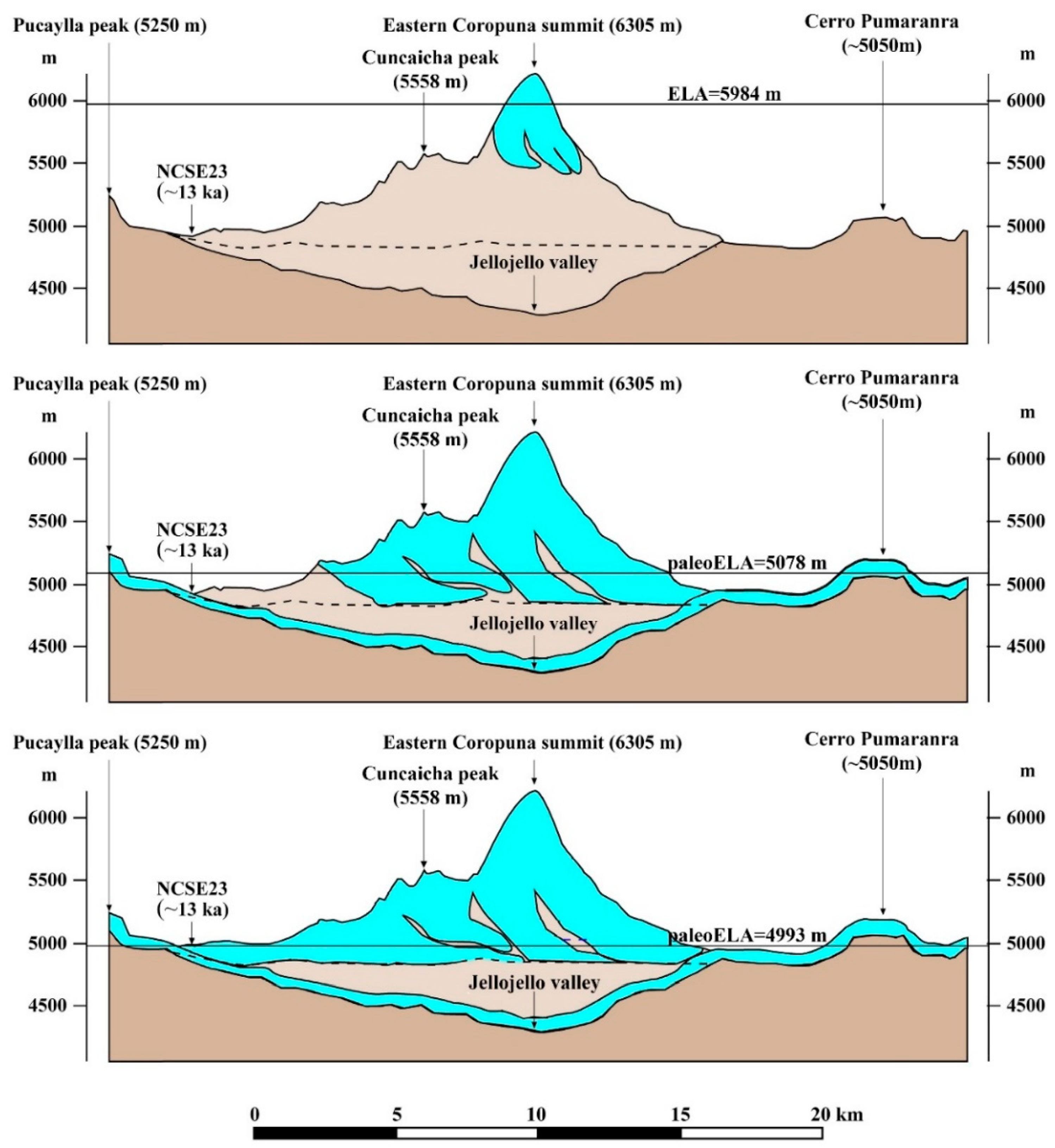
PaleoELA₁ = 5078 m: glaciers in maximum extension, from the highest mountains (eastern Coropuna summit and Cuncaicha Peak).

(b)

PaleoELA₂ = 4993 m: all mapped glaciers in maximum extension.

The paleoELA depression estimate, that is, its difference in altitude (m) with respect to the ELA₂₀₁₀, enabled the evaluation of the paleoclimate cooling with respect to the present, in the same phases (

Table 5. ELA depression and climate cooling.

ELA 2010 (m)	5984
BR	1.0
σ	96
PaleoELA (m)	PaleoELA1		PaleoELA2
	5078		4993
BR	3.0		3.0
σ	108		114
ΔELA (m)	907		991
ATLR (°C/km)	−6.5	−7.0	−6.5	−7.0
ΔT (°C)	ΔT1A	ΔT1B	ΔT2A	ΔT2B
	−5.9	−6.4	−6.4	−6.9

):

(a)

By analyzing the highest paleoglaciers (paleoELA₁ = 5078 m) we obtained: the paleoELA depression ΔELA₁ = −906 m and the climate cooling ΔT_1A = −5.9 °C, using the ATLR_EARTH = 6.5 °C/km and ΔT_1B = −6.4 °C, applying the current gradient ATLR₂₀₁₀ = 7.0 °C/km.

(b)

Through the analysis of all the paleoglaciers of the study area (paleoELA₂ = 4993 m), we estimated the paleoELA depression ΔELA₁ = −991 m and the climate cooling ΔT_2A = −6.4 °C, using the mean gradient ATLR_EARTH = 6.5 °C/km and ΔT_2B = −6.9 °C and the current gradient ATLR₂₀₁₀ = 7.0 °C/km.

Finally, the availability of paleoELA₂ and the cooling ΔT₂, served to evaluate the paleoprecipitation at 6080 m, the ice core altitude [59], for two ATLR values (

Table 6. Paleoprecipitation at the time of maximum glacial extension. Fz₂₀₁₀ was deducted from the data 1 January 2010–31 December 2010 recorded by CRYOPERU thermometers. Ice core data from Herreros et al. [59].

Present	2010 Freezing altitude annual average (Fz2010)		5589 m
	Previous 38 years accumulation at ice core level (6080 m)		580 mm
Glacier Last Maximum Extension	ATLR = 7.0 °C/km	Paleoprecipitation at ice core level	669 mm
		ΔP compared to present	15%	×1.2
	ATLR = 6.5 °C/km	Paleoprecipitation at ice core level	1628 mm
		ΔP compared to present	181%	×2.8

):

(a)

Assuming a value similar to the current ATLR₂₀₁₀ = 7.0 °C/km, a paleoprecipitation P_6080m = 669 mm was calculated (15% or ×1.2 higher than at present).

(b)

By applying the Earth mean value (ATLR_EARTH = 6.5 °C/km) a paleoprecipitation P_6080m = 1628 mm was estimated to be 181% or ×2.8 higher than at present.

5. Discussion

5.1. ELA, PaleoELA and Paleoclimate Reconstructions

The ELA, paleoELAs and their depression estimates are key aspects in this work and similar research, because they are the way to make paleoclimatic reconstructions and also to establish correlations to other proxy data.

5.1.1. ELA₂₀₁₀

The observable snowline altitude on the glaciers in 2010 averages about 6000 m (Figure 9), which could validate the data in Table 2. The difference between the ELA₂₀₁₀ (5915 ± 44 m) of Bromley et al. [47] and the ELA₂₀₁₀ (5984 m) reconstructed in this work is not very large and can be attributed to the data sources and the reconstruction methods used:

-

Both works used the elevation model of the national topographic map of Peru (IGN, scale 1: 50,000 and 50 m between contour lines), based on aerial photographs from 1955.

-

We have developed a reliable model, combining a 2010 satellite image with the contour lines, to apply the AABR method for the ELA and paleoELA reconstructions.

-

Bromley et al. [47] calculated the ELA₂₀₁₀ adding to the kinematic ELA₁₉₅₅, understood as the inflection from convex (ablation zone) to concave (accumulation zone) on the glacier surface contours (e.g., [91,92,93,94]), an assumed ELA_1955–2010 rise (m), deduced from three variables: Time elapsed from 1955 to 2010 (55 years); Air temperature warming in the Andes: 0.1 °C/decade [95] and the ATLR = 6.58 °C/km.

5.1.2. PaleoELA

From a geomorphological (non-chronological) point of view, the paleoELA for their CI phase calculated by Bromley et al. [47] is equivalent to the paleoELA₁ of this work. In both cases they are paleoELAs from glaciers at their maximum extension, although Bromley et al. [47] focused only on the glaciers that originated from the very Coropuna and Cuncaicha summits (source areas >5250 m; Figure 7) and we have analyzed ice flows from lower sites (<5250 m). Maybe that is why our paleoELA₁ (5078 m) is lower than the paleoELA_CI (5167 ± 59 m) from Bromley et al. [47].

The discrepancies are due to the different data and methods used: Maximum Elevation of Lateral Moraines (MELM; [96,97]) and THAR methods in Bromley et al. [47], and the AABR method in this work. Previous works highlighted that the AABR method creates better reconstructions than the other methods and is the only one that can be applied to current glaciers and paleoglaciers [75,81]. On the other hand, the paleoELA₂ (4993 m) reconstructed in this work can be a representative reconstruction of the maximum extension of all the paleoglaciers towards the Nevado Coropuna northeast (Figure 7), including the ice masses located in sites isolated topographically from the surrounding peaks. In addition, the paleoELA₂ allows us to calculate the deepest paleoELA depression in the mapped area (Figure 4), because Bromley et al. [47] only reconstructed paleoELAs from glaciers connected to the higher summits (>5250 m) and the paleoELA₂ is statistically representative of all paleoglaciers (source areas <5250 m).

5.1.3. PaleoELA Depression

The paleoELA depression (907–991 m, Table 6) estimated in this work is a little greater than the Bromley et al. [47] results (ΔELA = 748 ± 103). Anew, these differences can be attributed to the different methods used to reconstruct current and past ELAs. Besides, their interpretation is also different. While the paleoELA depression calculated by Bromley et al. [47] refers to maximum advances in valleys connected to the Coropuna peaks (CI phase), our estimate would be the maximum possible paleoELA depression in the study area, that is, the one that would take place during each phase of maximum glacier extension, which would be geomorphologically equivalent to the pre-CI phase of Bromley et al. [47].

5.1.4. Paleoclimate Reconstructions

A lot of evidence (e.g., [10,11]) suggests that, in the past, the climate in the Arid Tropical Andes was moister than in the present, which would have caused a lower ATLR. Thereupon, our cooling estimate using the global average ATLR_EARTH (6.5 °C/km) appears more probable than the estimate reached using the current ATLR₂₀₁₀ = 7.0 °C/km, which can be discarded.

Nonetheless, Bromley et al. [47] assumed a past precipitacion in Coropuna similar to the present, with the ATRL = 6–7 °C/km. From these premises and their paleoELA depression calculation (748 ± 103 m), they estimated that the paleoclimate was 4.9–5.6 °C colder than at present. Obviously it should be considered only for the CI phase of Bromley et al. [37], and therefore compared to the cooling deduced from our paleoELA₁ (higher glaciers). The cooling suggested by Bromley et al. [47] is 1.0–0.3 °C warmer than ours (5.9 °C) for the same phase.

However, our cooling (6.5 °C) and paleoprecipitation (15–181% or ×1.2–2.8 higher than the present climate) reconstructions are very similar to the results deduced in Cerro Tunupa, where a cooling of ~6.5 °C and a precipitation ×1.6–3.0 higher than in the present were estimated [8]. In any case, it is necessary to apply the procedures in new areas of study, which could allow us to fully discern the unknowns, which many parameters involved still pose, such as ATLR, different methods for ELA and paleotemperature reconstructions or current climate data shortage.

5.2. Geomorphological and Exposure Ages Interpretation

The ³⁶Cl ages presented in this work can only be interpreted as a preliminary prospecting, in a very complex study area. However, some ideas can be proposed to orient future research.

5.2.1. The Glaciers Maximum Extension and the Polygenic Moraines Deposition

Many of the mapped moraines are stacked forming sets (Figure 4) suggesting that the meeting of glaciers on the Altiplano resulted in the polygenic moraines, following the “obliterative overlap model” [98]. Glacial advances observed in Scandinavia in the decade of the 1990s of the 20th century had similar consequences. Depending on the valley, the glaciers carried and deposited six moraines or only one, as a result of the aggregation of different deposits by successive glacial advances [99]. Different works have pointed out interferences in glacial ages due to the aggregation of moraines, in Alaska [99], the Fennoscandian ice sheet [100] or the Carpathians [101].

These interferences could be even greater northeastward of Coropuna, because the same process could have been repeated many times over tens of thousands of years, as suggested by the following facts:

(a)

The high altitude of the stratovolcanoes (>6000 m) and the Altiplano (~4900–4700 m).

(b)

The paleoELA depression very close to the Altiplano level (paleoELA₂ = 4993 m).

(c)

The role of the Altiplano surrounding the mountains, behaving as a topographical obstacle to glacial advances.

(d)

The greater sensitivity of glaciers to precipitation than temperature [4].

(e)

The moister and colder paleoclimate than the present.

It is feasible that the joint action of these factors would result in the Coropuna glaciers achieving a steady state for a long time, close to the maximum advance. This could have happened during the Last Glacial Maximum (LGM) understood as the minimum relative sea level (RSL; ~26–19 ka ago; [102,103,104]). Likewise, even tens of thousands of years before the LGM, the ITCZ southward shift [13] and the paleolake transgressions on the Bolivian Altiplano [10,11] reveal a humid and favorable paleoclimate. That could have led to glacier advances (or a prolonged steady state in maximum extension) linked to boreal cooling episodes. If so, earlier large extension phases in the Coropuna glacier-system could also occur in marine isotope stages MIS3 and MIS4, which could explain the ³He ages classified as outliers [37] in the Huayllaura (towards the southwest) and Sigue Chico (westward of the Coropuna) valleys: ~61 and ~37 ka (Lm) or ~47 and ~31 ka (Li), respectively.

Furthermore, the topographic barriers imposed by pre-existing moraines and the surface of the Altiplano, which limited the ELA depression and the subsequent glacier growth down valley (Figure 4), would have obstructed glacier flow and created an almost permanent ice sheet. The combination of all these climatic and geomorphological factors may have resulted in a continuous glacier sedimentary action. That is, in the deposit of polygenic moraines which reflect several climate oscillations, all of approximately the same magnitude, and/or limited in size by topographic barriers. Both causes would have had the same effect: the prolongation of the maximum glaciers expansion phase. These processes would give a wide range of possible exposure ages. Therefore, the ³⁶Cl ages dispersion could be explained by both climatic oscillations and the existence of a topographic barrier. Taken together they could be interpreted as the result of large glacial advances, or glacial standstill over a long period of time. If this approach is correct, the west-east prospecting presented in this work would have detected these signals in all the sites sampled:

-

Eastern lateral moraine in Santiago Valley: sample NCNE01 (~14–11 ka).

-

Eastern lateral moraine in Queñua Ranra Valley: sample NCNE02 (~20–16 ka).

-

Western lateral moraine and terminal moraine in Pomullca valley: samples NCNE04 (~28–14 ka) and NCNE05 (~21–16 ka).

-

Terminal moraine deposited in Pampa Pucaylla Altiplano by paleoglaciers from the Pumaranra volcano-plateau: sample NCNE05 (~21–16 ka).

The polygenic moraines hypothesis could also explain the dispersion in four ³He-Lm/³He-Li ages [37] in the Mapa Mayo valley, NC1 (~21/~17 ka), NC2 (~16/~13 ka), NC3 (~15/~12 ka) and NC4 (~25/~20 ka), as well as the differences between two ³He-Li ages (NC9 and NC10; ~17 ka; [37]) and our NCNE01 ³⁶Cl age (~12 ka), on three moraine boulders in Santiago Valley. It is possible that NC9 and NC10 are dating 1–2 older advances and NCNE01 a younger advance, which reached the same place and added a new moraine to pre-existing moraines. The younger moraines aggregation on older moraines, could also be the cause of the dispersed ages in many Andean glacial sites, such as Cajamarca [45], Cordillera Blanca [29], Jeulla Raju [105], Huayhuash [106], Junín [28], Quelccaya ice cap [6,107], Carabaya [46], Huayna Potosí, Río Suturi and Huamaní Loma [39]; Coropuna [37,38]; (this work); Hualca Hualca [7], Cerro Tunupa [8], and Uturuncu volcano [9].

5.2.2. The Deglaciation Onset in the Nevado Coropuna and Its Surroundings

The NCSE23, NCNE08 and NCNE09 ages pose a problem, because they indicate two apparently contradictory simultaneous events: deglaciation in the Pampa Pucaylla Altiplano (~4900 m in altitude) and large glacial advances in the bottom of the Jellojello Valley (~4100 m). However, this apparent paradox could be explained, jointly or separately, by any of the following causes:

(a)

The sampled surfaces rejuvenation by erosion (NCNE08 and NCNE09). It is a feasible hypothesis, although the preservation of abundant polished bedrocks on the Nevado Coropuna southern and western slopes [51] suggests that erosion rates may have been very low.

(b)

The volcanic activity and geothermal heat’s influence on deglaciation. This is also possible, as indicated by the following facts:

-

West, southeast and northeast of the Coropuna summits, three clearly postglacial lava flows (Figure 1), the last one only 2 ka ago (sample NCNE03), are evidence that Coropuna is not an extinct volcano.

-

Around the Coropuna there are lower sites (~5200 m), where the presence of permafrost has been detected and is being monitored [108], and higher sites (~5700 m), where the thermometers buried in moraines which overlie the Queñua Ranra lava flow, have barely registered freezing episodes [51].

-

Regardless of the altitude, if the distribution of ground temperature was also unequal in the past, it could have caused the deglaciation of some places, while at other sites glacial advances could occur.

(c)

The paleoELA reconstructions show accumulation areas in the Jellojello and Ccallhua Valleys headwaters (Figure 7), whether they are calculated considering only the glaciers coming from the highest mountains (paleoELA₁ = 5078 m), or if they are estimated for all the mapped ice masses (paleoELA₂ = 4993 m).

The paleoELA₁ would imply the disappearance of the accumulation zones in the Pampa Pucaylla Altiplano, where the NCSE23 sample was collected. It is a site topographically disconnected from the surrounding peaks, where the glaciers went down from a nearby low hill (Figure 4, Figure 9 and Figure 10). Therefore, a paleoELA ranging 5078–4993 m could have caused, at the same time, the deglaciation of that site in the Pampa Pucaylla Altiplano and advances (or glacial standstill) into the Jellojello Valley (Figure 11).

In our study area, the timing of the deglaciation remains still unknown, due to the scarcity of ages and the geomorphological complexity of the Coropuna-altiplano-lower valleys interface. However, besides the NCSE23 age (15.0–11.0 ka), three facts suggest that the retreat could have started after ~12 ka and before ~9 ka:

-

The NCNE01 sample seems to indicate a maximum advance in the Santiago Valley 13.6–11.0 ka ago.

-

In the Jellojello Valley there are moraines even younger than those dating from 14.6 to 9.8 ka, according to the NCNE08 and NCNE09 ages.

-

The NCNE06 sample suggests that, 10.7–8.1 ka ago, a glacier existed that only reached the middle part of the Huajra Huire valley, which indicates that by that time the deglaciation had already begun and was quite significant (Figure 4).

The exposure ages of the polished bedrocks at different altitudes on the Coropuna southern and western slopes will help calculate the timing of deglaciation. The authors of this work are preparing a new study on this interesting subject. Meanwhile, the ages calculated by Alcalá-Reygosa et al. [7] using the same isotope and protocol for sample preparation as us, are compatible with the deglaciation onset ~15–10 ka ago:

-

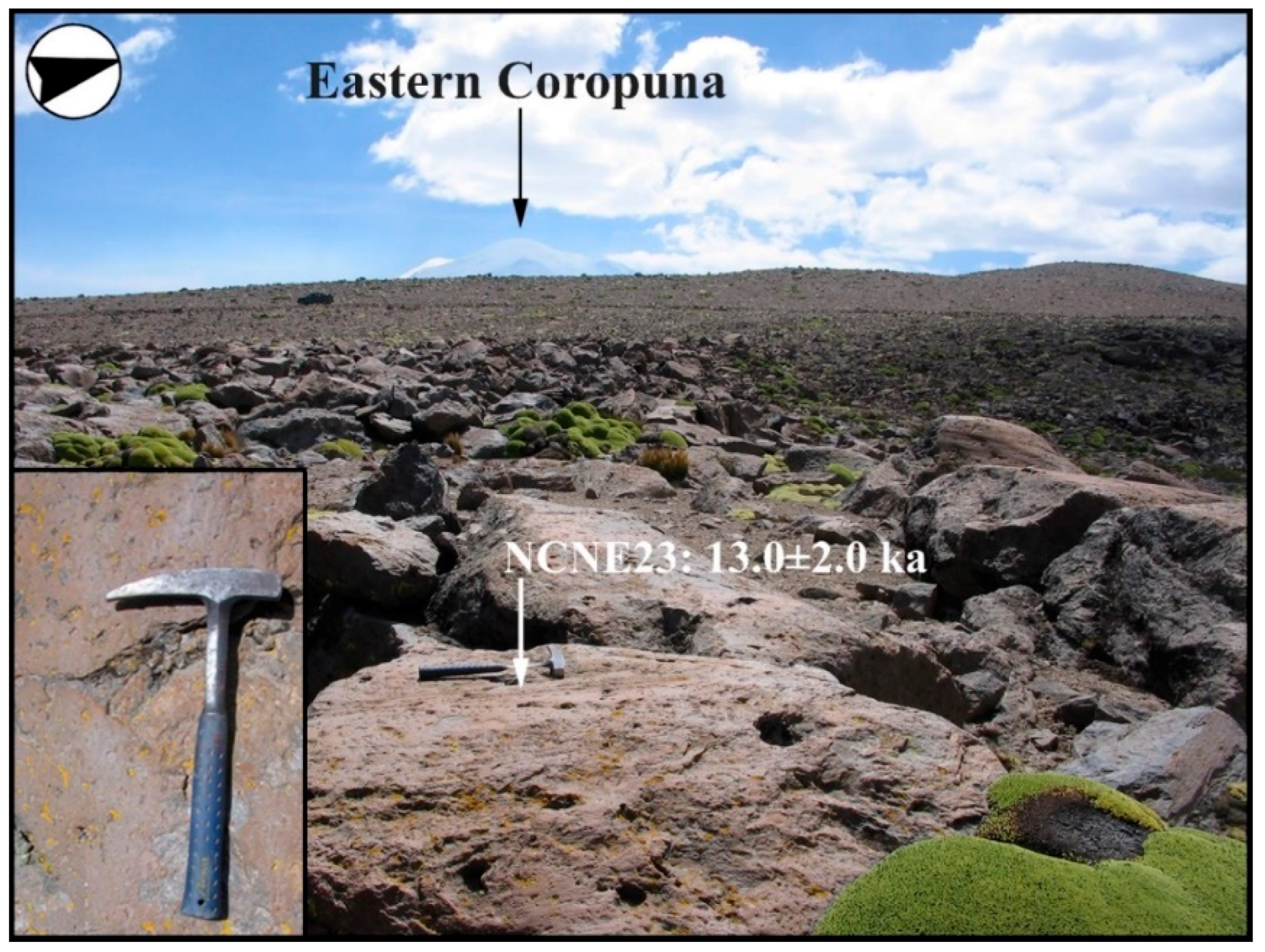
On the Altiplano, ~20 km eastward of the Hualca Hualca stratovolcano, the Patapampa 4 sample (a polished bedrock) suggests that, in the lowest places, topographically isolated from the surrounding peaks, the melting could have begun 12.9–10.9 ka ago.

-

Although there is some uncertainty due to the error ranges, the sample comes from a similar geomorphological framework, an Altiplano site at 4886 m in altitude cut off from higher mountains, and the chronology is quite consistent with our NCSE23 age (13.0 ± 2.0 ka).

-

The Pujro Huayjo 2 was collected from another polished bedrock, at low altitude (4450 m) but coming from a higher source area, the Hualca Hualca summit (~5800 m). Despite that, the age (13.9–9.1 ka) is not absolutely incompatible with the Patapampa 4 and our Coropuna ages (like NCSE23).

The next question to be resolved is whether this evidence is consistent with regional and global paleoclimatic data.

5.3. Paleoclimatic Framework

Solid or liquid precipitation produces different effects in the glacier mass balance. Similarly, the ITCZ southward shift also influences differently in the Andean glaciers, positively (if it snows) or negatively (if it rains). Therefore, after the LGM-RSL, the Central Andes deglaciation onset could have happened earlier or later, depending on the temperature evolution in both terrestrial hemispheres (Figure 12):

(a)

First, between ~19 and ~9 ka, the Surface Sea Temperature (SST) westward of the Iberian Peninsula (SSTN; [109]) got warmer by 6 °C in 10 ka. However, it was not a gradual trend, because it was broken by abrupt cold episodes due to AMOC shutdowns: H1 (e.g., [110,111]) and YD (e.g., [112]), which appear reflected in the SST_N curve, ~18 and ~12 ka ago, respectively.

(b)

Secondly, the humidity increases due to cold boreal events, which is well recorded in the Andean Altiplano lacustrine evidence; e.g.,

-

At the Coropuna latitude (~16° S), one clear evidence of moister conditions is the strong decrease in the Titicaca salinity ~21–10 ka ago, as shown by the great abundance (>80%) of freshwater plankton, nowadays extinct, in the lake sediments [113].

-

Southward (17–22° S), in the lake transgressions Sajsi (~25–19 ka); Tauca (~18–14 ka) and Coipasa (~11–13 ka; [10]). The wettest climate was at the Tauca highstand (17.0–15.7 ka). The maximum water depth of 120 m was registered in the center of the Uyuni basin, for a total lake surface of about 52.000 km² [8,10,114,115].

Throughout the same period (~19–9 ka), in the southern coast of Chile (SST_S [116]) the warming is equivalent to that observed in the Northern Hemisphere (6 °C/10 ka). However, it is an uninterrupted trend with only one exception, a brief attenuation in warming, the slight cooling around ~14 ka, which could reflect the Atlantic Cold Reversal (ACR; e.g., [117]). It is possible that the episodes of boreal cooling associated with AMOC shutdowns, through the ITCZ southward deflection and/or the SASM reinforcement, have allowed the conservation of the Central Andes highest glaciers after the LGM-RSL. However, this must have been a phenomenon restricted to the sites that met ideal conditions, in altitude and latitude, factors that should be taken into accounts to understand the glacial ages on regional and local scales:

(a)

The mountain altitude determines which areas can be higher and colder than the isotherm of air temperature of 0 °C, transforming into places where:

-

Precipitation is exclusively solid (as it still happens nowadays in Coropuna) and do not negatively influence the glaciers mass balance.

-

The snow is preserved and transformed into glacier ice, feeding a positive mass balance.

(b)

The mountains latitude is also key, due to the climate dryness trend to increase westward and southward of the Central Andes, and the ELA rise in the same direction, because of the aridity [25]. As an outcome of this trend, southern of the South American Arid Diagonal, there are currently no glaciers in mountains as high as Uturuncu volcano (~22° S, 6009 m) or Nevado Ojos del Salado (~27° S, 6893 m).

5.4. The Last Glacial Maximum and Deglaciation in the Arid Tropical Andes

Despite the climatic data scarcity, especially in the higher mountains, the annual total precipitation estimates show an increase in aridity towards the south of the Arid Tropical Andes. These estimates range from ~700–500 mm/year [118]; (Figure 3) in the Coropuna and Hualca Hualca latitude (~16° S) to ~300–200 mm/year in Nevado Sajama (~18° S) and ~200 mm/year in Tunupa (~20°; [10,119]), reaching the maximum regional dryness on the Uturuncu Volcano (~22° S), <100 mm/year [10,120], near the southern tropics limits. The available glacial ages (Figure 13 and Figure 14) from the Arid Tropical Andes [7,8,9,121]; (this work) are consistent with the southward increase in aridity and ELA.

The absolute datings showing the deglaciation onset (recessional moraines and/or polished bedrocks) are earlier in the southernmost mountains, which are drier and further from the influence of tropical circulation, and more recent in the more northern and less arid mountains, as they are closer to the tropical circulation, as discussed below:

In the southern mountains, the ³He ages suggest maximum glacier extent episodes as early as ~65, ~40 and ~35–17 ka, in Uturuncu [9] and ~170–130 ka (previous to the last glacial cycle) and ~23–17 ka in Tunupa [8]. These works identified standstill glaciers near their maximum extension, synchronous with the Tauca highstand (~17–15 ka), and then a quick deglaciation towards the summit area:

-

In Uturuncu (~22° S) the glaciers retreated higher than 5094–5111 m in altitude, ~16.1–13.7 ka ago (polished bedrock ages for UTU-1A, UTU-1B and UTU-1C). Given that the glacial shrinkage was synchronous to the Bølling-Allerød (B/A) boreal warming, it could reflect a mixed influence of the regional temperature increase, together with the abrupt oscillations of late Pleistocene precipitation, at the rate of the North Atlantic events [9].

-

In Cerro Tunupa (~20° S), there was also a fast deglaciation, after the Tauca highstand and contemporaneous with the B/A boreal warming. Despite the lower Tunupa altitude (~5400 m), compared to Uturuncu (6009 m), it seems that the greater closeness of tropical circulation (Tunupa is ~280 km northward of Uturuncu) enabled a small glacier pulse, ~13.6–11.8 ka ago (moraine ages TU-3A and TU-3B), during the paleolake Coipasa transgression (Figure 12) and the boreal YD, and before the complete Tunupa deglaciation, after ~12 ka [9].

The Tunupa-Coropuna comparison allows to suggest some hypotheses:

-

The last glacier pulse in Tunupa seems synchronous with our observations eastward of Coropuna ~14.6–9.8 ka (moraine ages for NCNE08 and NCNE09), when glaciers overflowed the Pampa Pucaylla Altiplano and went down the Ccallhua and Jellojello Valleys. In both cases (Tunupa and Pampa Pucaylla) the glaciers came from the same summit altitude (~5100 m), which point out that our reconstructions in Coropuna (Figure 11) are a regional paleoELA good estimate (~5078–4993 m).

-

The divergences in magnitude (maximum advances in Coropuna and small late pulse in Tunupa) could be due to the differences in latitude and altitude, because Coropuna is higher and further to the North and Tunupa’s lower and further to the South, so there is another possibility: the boreal warming B/A would have weakened the tropical circulation, retracting its influence area towards a lower latitude. This way would explain why they occurred simultaneously: great freshwater plankton abundance (90%) in Lake Titicaca sediments [113]; Figure 12), long glacial standstill episodes in the Ccallhua and Jellojello valleys, lower than the altiplano (this work), both at ~16° S, and the glacier pulse in Tunupa, smaller and closer to the summit [8], at ~20° S.

Likewise, it is possible to find Sajama-Coropuna correlations that align with previous hypotheses. Sajama (~18° S) is a volcano located ~220 km toward north of Tunupa, and therefore, closer to the influence of tropical circulation. Besides, Sajama is the highest mountain in the Arid Tropical Andes (6542 m). Perhaps for both reasons, the southernmost current-glacier in the region is on the Sajama summit. Like with Uturuncu, the ages of polished bedrocks in Sajama (Figure 13 and Figure 14) also suggest a maximum glacier extent prior to the LGM-RSL (e.g., the BV-06-06 age, ~28 ka), and ice tongues reaching the Altiplano in the stratovolcano surroundings, just as it happened northeastward of Coropuna.

Moreover, the highest polished bedrock ages in Sajama (BV-06-20, BV-06-21 and BV-06-22), show a fairly advanced phase in the deglaciation process: the glaciers retreat in the Patohko Valley, ~13.8–9.9 ka ago. However, ~400–500 km northwestward of Sajama, other polished bedrock ages suggest that, at that same time, the deglaciation only was in its onset, in two Altiplano sites (at ~16° S latitude), separated by 100 km away: the Patapampa 4 age (11.9 ± 1.0 ka; [7],), in the Patapampa Altiplano, eastward of the Hualca Hualca Volcano, and the NCSE23 age (13.0 ± 2.0 ka); (this work), in the Pampa Pucaylla Altiplano, towards the east of Coropuna. In the Sajama, Patapampa and Pampa Pucaylla practically simultaneous symptoms of deglaciation are observed (at millennial scales), although they must be differently interpreted:

-

On Patapampa and Pucaylla, the glaciers disappear in lower sites (~4900 m), topographically isolated from higher peaks.

-

In Patohko, glaciers linked to the summit area of Sajama (6542 m) retreated up the slope from the middle valley (4692–4712 m).

These discrepancies could also confirm (as other evidence discussed above) that altitude and latitude modulate the tropical circulation influence and are therefore key factors in explaining glacial expansion in the Arid Tropical Andes. Taking these premises into account, it is possible that the deglaciation began earlier in the Southern Altiplano, most arid and further away from the tropical circulation source area, and then spread to lower latitudes, with local effects depended on altitude and latitude. Although with some uncertainties, we believe that the proposed ideas construct a coherent regional interpretation, explaining the ³He and ³⁶Cl ages reasonably from Coropuna, Hualca Hualca and their surroundings ([7,37]; this work), as well as the other glacial chronologies available from the Arid Tropical Andes: Sajama [121], Tunupa [8] and Uturuncu [9]. The glacial ages and paleoclimatic proxies seem consistent with evidence showing a link between tropical glaciers and the Northern Hemisphere cooling episodes, through the tropical circulation southward shift [20,21,22,23,24].

6. Conclusions

-

A ³⁶Cl glacial ages survey and a paleoclimatic reconstruction based on the geomorphological evidence of the glaciers past evolution has been achieved on Nevado Coropuna. The results have been compared to information of the same type obtained by previous works in other Andean mountains, as well as to other present and past evidences on the regional climate and its global teleconnections.

-

According to our data set interpretation, the Nevado Coropuna glacier system may have been near or in maximum expansion along the MIS2, MIS3, and MIS4 marine isotope stages and even earlier. During this timespan, it is possible that many glacial advances occurred, which reached the same extent as a result of the damming effect of pre-existing moraines and the role of the Altiplano as a topographic barrier. It is also possible that the glaciers had been in a steady state close to their maximum extension for a long time. Any of the two possibilities (multiple large advances and/or long glacial standstill) could explain, jointly or separately, that nowadays we find polygenic moraines, which can include a wide range of exposure ages. The polygenic moraines diachronic deposition can also explain the glacial ages dispersion in other Tropical Andes mountains.

-

The Coropuna and other mountains glacial ages indicate more humid climate conditions than the currently Arid Tropical Andes, possibly linked to the Northern Hemisphere cooling episodes via the tropical circulation southward shift. The relational boreal cooling-tropical humidity-Andean glaciers extension may have happened along the last glacial cycle and also in previous glacial cycles. Likewise, it must be the cause of the conservation, in the Coropuna and other mountains, of great advances (or glacial standstill) after the LGM ended and until the last lake transgressions in the Bolivian Altiplano.

-

The increased aridity demonstrated by the ELA trend south of the region indicates that the mountains latitude and altitude must have a very important role in the glaciers evolution on the Arid Tropical Andes, modulating the glacial response to changes in tropical circulation and boreal cooling. For this reason, the last regional deglaciation seems to have been earlier in the southernmost, driest, and/or lower mountains and more belated in the northernmost, less arid and higher mountains.

References

1. Kaser, G.; Osmaston, H. Tropical Glaciers; Cambridge University Press: Cambridge, UK, 2002; p. 207. [Google Scholar]
2. Rupper, S.; Roe, G.; Gillespie, A. Spatial patterns of Holocene glacier advance and retreat in Central Asia. Quat. Res. 2009, 72, 337–346. [Google Scholar] [CrossRef]
3. Rupper, S.; Roe, G. Glacier changes and regional climate: A mass and energy balance approach. J. Clim. 2008, 21, 5384–5401. [Google Scholar] [CrossRef]
4. Sagredo, E.A.; Rupper, S.; Lowell, T.V. Sensitivities of the equilibrium line altitude to temperature and precipitation changes along the Andes. Quat. Res. 2014, 81, 355–366. [Google Scholar] [CrossRef]
5. Sagredo, E.; Lowell, T. Climatology of Andean glaciers: A framework to understand glacier response to climate change. Glob. Planet. Chang. 2012, 86–87, 101–109. [Google Scholar] [CrossRef]
6. Kelly, M.A.; Lowell, T.V.; Applegate, P.J.; Smith, C.A.; Phillips, F.M.; Hudson, M.A. Late glacial fluctuations of Quelccaya Ice Cap, southeastern Peru. Geology 2012, 40, 991–994. [Google Scholar] [CrossRef]
7. Alcalá-Reygosa, J.; Palacios, D.; Vázquez-Selem, J. A preliminary investigation of the timing of the local last glacial maximum and deglaciation on HualcaHualca volcano-Patapampa Altiplano (arid Central Andes, Peru). Quat. Int. 2017, 449, 149–160. [Google Scholar] [CrossRef]
8. Blard, P.-H.; Lavé, J.; Farley, K.A.; Fornari, M.; Jiménez, N.; Ramirez, V. Late local glacial maximum in the Central Altiplano triggered by cold and locally-wet conditions during the paleolake Tauca episode (17–15 ka, Heinrich 1). Quat. Sci. Rev. 2009, 28, 3414–3427. [Google Scholar] [CrossRef]
9. Blard, P.-H.; Lavé, J.; Farley, K.A.; Ramírez, V.; Jiménez, N.; Martin, L.C.P.; Charreau, J.; Tibari, B.; Fornari, M. Progressive glacial retreat in the Southern Altiplano (Uturuncu volcano, 22° S) between 65 and 14 ka constrained by cosmogenic 3He dating. Quat. Res. 2014, 82, 209–221. [Google Scholar] [CrossRef]
10. Blard, P.-H.; Sylvestre, F.; Tripati, A.K.; Claude, C.; Causse, C.; Coudraing, A.; Condom, T.; Seidel, J.-L.; Vimeux, F.; Moreau, C.; et al. Lake highstands on the Altiplano (Tropical Andes) contemporaneous with Heinrich 1 and the Younger Dryas: New insights from 14C, U-Th dating and d18O of carbonates. Quat. Sci. Rev. 2011, 30, 3973–3989. [Google Scholar] [CrossRef]
11. Placzek, C.J.; Quade, J.; Patchett, P.J. A 130 ka reconstruction of rainfall on the Bolivian Altiplano. Earth Planet. Sci. Lett. 2013, 363, 97–108. [Google Scholar] [CrossRef]
12. Sachs, J.P.; Sachse, D.; Smittenberg, R.H.; Zhang, Z.; Battisti, D.S.; Golubic, S. Southward movement of the Pacific intertropical convergence zone AD 1400–1850. Nat. Geosci. 2009, 554, 1–7. [Google Scholar] [CrossRef]
13. Schneider, T.; Bischoff, T.; Haug, G.H. Migrations and dynamics of the intertropical convergence zone. Nature 2014, 513, 45–53. [Google Scholar] [CrossRef] [PubMed]
14. Wang, X.; Auler, A.S.; Edwards, R.L.; Cheng, H.; Cristalli, P.S.; Smart, P.L.; Richards, D.A.; Shen, C.-C. Wet periods in northeastern Brazil over the past 210 kyr linked to distant climate anomalies. Nature 2004, 432, 740–743. [Google Scholar] [CrossRef] [PubMed]
15. Apaéstegui, J.; Cruz, F.W.; Vuille, M.; Fohlmeistere, J.; Espinoza, J.C.; Sifeddineg, A.; Strikish, N.; Guyot, J.L.; Ventura, R.; Chengk, H.; et al. Precipitation changes over the eastern Bolivian Andes inferred from speleothem (δ18O) records for the last 1400 years. Earth Planet. Sci. Lett. 2018, 494, 124–134. [Google Scholar] [CrossRef]
16. Thompson, L.G.; Mosley-Thompson, E.; Henderson, K.A. Ice-core palaeoclimate records in tropical South America since the Last Glacial Maximum. J. Quat. Sci. 2000, 15, 377–394. [Google Scholar] [CrossRef] [Green Version]
17. Peterson, L.C.; Haug, G.H.; Hughen, K.A.; Röhl, U. Rapid Changes in the Hydrologic Cycle of the Tropical Atlantic During the Last Glacial. Science 2001, 290, 1947–1951. [Google Scholar] [CrossRef]
18. Haug, G.H.; Hughen, K.A.; Sigman, D.M.; Peterson, L.C.; Röhl, U. Southward Migration of the ITCZ Through the Holocene. Science 2001, 293, 1304–1308. [Google Scholar] [CrossRef] [PubMed]
19. Wanner, H.; Beer, J.; Bütikofer, J.; Crowley, T.J.; Cubasch, U.; Flückiger, J.; Goosse, H.; Grosjean, M.; Joos, F.; Kaplan, J.O.; et al. Mid- to Late Holocene climate change: An overview. Quat. Sci. Rev. 2008, 27, 1791–1828. [Google Scholar] [CrossRef]
20. Chiang, J.C.H.; Bitz, C.M. Influence of high latitude ice cover on the marine Intertropical Convergence Zone. Clim. Dyn. 2005, 25, 477–496. [Google Scholar] [CrossRef]
21. Zhang, R.; Delworth, T.L. Simulated tropical response to a substantial weakening of the Atlantic thermohaline circulation. J. Clim. 2005, 18, 1853–1860. [Google Scholar] [CrossRef]
22. Broccoli, A.J.; Dahl, K.A.; Stouffer, R.J. Response of the ITCZ to Northern Hemisphere cooling. Geophys. Res. Lett. 2006, 33, 1–4. [Google Scholar] [CrossRef]
23. Chiang, J.C.H.; Biasutti, M.; Battisti, D.S. Sensitivity of the Atlantic Intertropical Convergence Zone to Last Glacial Maximum boundary conditions. Palaeogeography 2003, 18, 1–18. [Google Scholar] [CrossRef]
24. Chiang, J.C.H.; Friedman, A.R. Extratropical cooling, interhemispheric thermal gradients, and tropical climate change. Annu. Rev. Earth Planet. Sci. 2012, 40, 383–412. [Google Scholar] [CrossRef]
25. Clapperton, C. Quaternary Geology and Geomorphology of South America; Elsevier: Amsterdam, The Netherlands, 1993; p. 769. [Google Scholar]
26. Balco, G. Contributions and unrealized potential contributions of cosmogenic-nuclide exposure dating to glacier chronology, 1990–2010. Quat. Sci. Rev. 2011, 30, 3–27. [Google Scholar] [CrossRef]
27. Mark, B.; Stansell, N.; Zeballos, G. The Last Deglaciation of Peru and Bolivia. Cuadernos de Investigación Geográfica 2017, 43, 591–628. [Google Scholar] [CrossRef]
28. Smith, J.A.; Seltzer, G.O.; Farber, D.L.; Rodbell, D.T.; Finkel, R.C. Early Local Last Glacial Maximum in the Tropical Andes. Science 2005, 308, 678–681. [Google Scholar] [CrossRef] [PubMed] [Green Version]
29. Farber, D.L.; Hancock, G.S.; Finkel, R.C.; Rodbell, D.T. The age and extent of tropical alpine glaciation in the Cordillera Blanca, Peru. J. Quat. Sci. 2005, 20, 759–776. [Google Scholar] [CrossRef]
30. Phillips, F.M.; Plummer, M.A. CHLOE: A program for interpreting in-situ cosmogenic nuclide dating and erosion studies (abs). Radiocarbon 1996, 38, 98. [Google Scholar]
31. Balco, G.; Stone, J.O.; Lifton, N.A.; Dunai, T.J. A complete and easily accessible means of calculating surface exposure ages or erosion rates from 10Be and 26Al measurements. Quat. Geochronol. 2008, 3, 174–195. [Google Scholar] [CrossRef]
32. Marrero, S.M.; Phillips, F.M.; Borchers, B.; Lifton, N.; Aumer, R.; Balco, G. Cosmogenic nuclide systematics and the CRONUScalc program. Quat. Geochronol. 2016, 31, 160–187. [Google Scholar] [CrossRef] [Green Version]
33. Marrero, S.; Phillips, F.; Caffee, M.; Gosse, J. CRONUS-Earth cosmogenic 36Cl calibration. Quat. Geochronol. 2015, 31, 199–219. [Google Scholar] [CrossRef]
34. Martin, L.C.P.; Blard, P.-H.; Balco, G.; Lavé, J.; Delunel, R.; Lifton, N.; Laurent, V. The CREp program and the ICE-D production rate calibration database: A fully parameterizable and updated online tool to compute cosmicray exposure ages. Quat. Geochronol. 2017, 38, 25–49. [Google Scholar] [CrossRef]
35. Schimmelpfennig, I.; Benedetti, L.; Finkel, R.; Pik, R.; Blard, P.H.; Bourle, D.; Burnard, P.; Williams, A. Sources of in-situ 36Cl in basaltic rocks. Implications for calibration of production rates. Quat. Geochronol. 2009, 4, 441–461. [Google Scholar] [CrossRef]
36. Vermeesch, P. CosmoCalc: An Excel add-in for cosmogenic nuclide calculations. Geochem. Geophys. Geosyst. 2007, 8, 1–14. [Google Scholar] [CrossRef]
37. Bromley, G.R.M.; Schaefer, J.M.; Winckler, G.; Hall, B.L.; Todd, C.E.; Rademaker, K.M. Relative timing of last glacial maximum and late-glacial events in the central tropical Andes. Quat. Sci. Rev. 2009, 1–13. [Google Scholar] [CrossRef]
38. Bromley, R.M.; Hall, B.L.; Schaefer, J.M.; Winckeler, G.; Todd, C.E.; Rademaker, K.M. Glacier fluctuations in the southern Peruvian Andes during the late-glacial period, constrained with cosmogenic 3He. J. Quat. Sci. 2011, 26, 37–43. [Google Scholar] [CrossRef]
39. Zech, R.; Kull, C.; Kubik, P.W.; Veit, H. LGM and Late Glacial glacier advances in the Cordillera Real and Cochabamba (Bolivia) deduced from 10Be surface exposure dating. Clim. Past Discuss. 2007, 3, 839–869. [Google Scholar] [CrossRef]
40. Zech, R.; May, J.-H.; Kull, C.; Ilgner, J.; Kubik, P.W.; Veit, H. Timing of the late Quaternary glaciation in the Andes from ~15° to 40° S. J. Quat. Sci. 2008, 23, 635–647. [Google Scholar] [CrossRef]
41. Smith, J.A.; Mark, B.G.; Rodbell, D.T. The timing and magnitude of mountain glaciation in the tropical Andes. J. Quat. Sci. 2008, 23, 609–634. [Google Scholar] [CrossRef]
42. Blard, P.-H.; Lavé, J.; Sylvestre, F.; Placzek, C.; Claude, C.; Galy, V.; Condom, T.; Tibari, B. Cosmogenic 3He production rate in the high tropical Andes (3800 m, 20° S): Implications for the local last glacial maximum. Earth Planet. Sci. Lett. 2013, 377–378, 260–275. [Google Scholar] [CrossRef]
43. Borchers, B.; Marrero, S.; Balco, G.; Caffee, M.; Goehring, B.M.; Lifton, N.; Nishiizumi, K.; Phillips, F.; Schaefer, J.; Stone, J. Geological calibration of spallation production rates in the CRONUSEarth project. Quat. Geochronol. 2016, 31, 188–198. [Google Scholar] [CrossRef]
44. Kelly, M.A.; Lowell, T.V.; Applegate, P.J.; Phillips, F.M.; Schaefer, J.M.; Smith, C.A.; Kim, H.; Leonard, K.C.; Hudson, A.M. A locally calibrated, late glacial 10Be production rate from a low-latitude, high-altitude site in the Peruvian Andes. Quat. Geochronoly 2015, 26, 70–85. [Google Scholar] [CrossRef]
45. Shakun, J.D.; Clark, P.U.; Marcott, S.A.; Brook, E.J.; Lifton, N.A.; Caffee, M.; Shakun, W.R. Cosmogenic dating of Late Pleistocene glaciation, southern tropical Andes, Peru. J. Quat. Sci. 2015, 30, 841–847. [Google Scholar] [CrossRef]
46. Bromley, G.R.M.; Schaefer, J.; Hall, B.L.; Rademaker, K.M.; Putnam, A.E.; Todd, C.E.; Hegland, M.; Winkler, G.; Jackson, M.S.; Strand, P.D. A cosmogenic 10Be chronology for the local last glacial maximum and termination in the Cordillera Oriental, southern Peruvian Andes: Implications for the tropical role in global climate. Quat. Sci. Rev. 2016, 148, 54–67. [Google Scholar] [CrossRef]
47. Bromley, R.M.; Hall, B.L.; Rademaker, K.M.; Todd, C.E.; Racoviteanu, A.E. Late Pleistocene snowline fluctuations at Nevado Coropuna (15° S), southern Peruvian Andes. J. Quat. Sci. 2011, 26, 305–317. [Google Scholar] [CrossRef]
48. Venturelli, G.; Fragipane, M.; Weibel, M.; Antiga, D. Trace element distribution in the Cenozoic lavas of Nevado Coropuna and Andagua Valley, Central Andes of southern Peru. Bull. Volcanol. 1978, 41, 213–228. [Google Scholar] [CrossRef]
49. Weibel, M.; Fejer, Z. El Nevado Coropuna, Departamento de Arequipa. Boletín de la Sociedad Geológica del Perú 1977, 57–58, 87–98. [Google Scholar]
50. Weibel, M.; Frangipane-Gysel, M.; Hunziker, J. Nevado Coropuna. Ein Beitrag zur Vulkanologie Süd-Perus. Geologische Rundschau 1978, 67, 243–252. [Google Scholar] [CrossRef]
51. Úbeda, J. El Impacto del Cambio Climático en los Glaciares del Complejo Volcánico Nevado Coropuna (Cordillera Occidental de los Andes, Sur del Perú). Ph.D. Thesis, Universidad Complutense de Madrid, Madrid, Spain, 2011. [Google Scholar]
52. Garreaud, R.D.; Vuille, M.; Compagnucci, R.; Marengo, J. Present-day South American climate. Palaeogeogr. Palaeoclimatol. Palaeoecol. 2009, 281, 180–195. [Google Scholar] [CrossRef]
53. Houston, J.; Hartley, A.J. The central Andean west-slope rainshadow and its potential contribution to the origin of hyper-aridity in the Atacama Desert. Int. J. Climatol. 2003, 23, 1453–1464. [Google Scholar] [CrossRef] [Green Version]
54. Garreaud, R.D.; Molina, A.; Farias, M. Andean uplift, ocean cooling and Atacama hyperaridity: A climate modeling perspective. Earth Planet. Sci. Lett. 2010, 292, 39–50. [Google Scholar] [CrossRef]
55. Sylvestre, F. Moisture Pattern during the Last Glacial Maximum in South America. In Past Climate Variability in South America and Surrounding Regions, Developments in Paleoenvironmental Research; Vimeux, F., Sylvestre, F., Khodri, M., Eds.; Springer: Berlin/Heidelberg, Germany, 2009; Volume 14, pp. 3–28. [Google Scholar]
56. Nogués-Paegle, J.; Mechoso, C.R.; Fu, R. Progress in Pan American CLIVAR Research: Understanding the South American Monsoon. Meteorologica 2002, 27, 3–30. [Google Scholar]
57. Vera, C.; Higgins, W.; Amador, J.; Ambrizzi, T.; Garreaud, R.; Gochis, D.; Gutzler, D.; Lettenmaier, D.; Marengo, J.; Mechoso, C.R.; et al. Toward a Unified View of the American Monsoon Systems. J. Clim. 2006, 19, 4977–5000. [Google Scholar] [CrossRef] [Green Version]
58. Zhou, J.; Lau, K.M. Does a monsoon climate exist over South America? J. Clim. 1998, 11, 1020–1040. [Google Scholar] [CrossRef]
59. Herreros, J.; Moreno, I.; Taupin, J.D. Environmental records from temperate glacier ice on Nevado Coropuna saddle, southern Peru. Adv. Geosci. 2009, 22, 27–34. [Google Scholar] [CrossRef] [Green Version]
60. Kuentz, A.; Galán De Mera, A.; Ledru, M.P.; Thouret, J.C. Phytogeographical data and modern pollen rain of the puna belt in southern Peru (Nevado Coropuna, Western Cordillera). J. Biogeogr. 2007, 34, 1762–1776. [Google Scholar] [CrossRef]
61. Kuentz, A.; Ledru, M.P.; Thouret, J.C. Environmental changes in the highlands of the western Andean Cordillera, southern Peru, during the Holocene. Holocene 2012, 22, 1215–1226. [Google Scholar] [CrossRef]
62. Hanshaw, M.N.; Bookhagen, B. Glacial areas, lake areas, and snow lines from 1975 to 2012: Status of the Cordillera Vilcanota, including the Quelccaya Ice Cap, northern central Andes, Peru. Cryosphere 2014, 8, 1–18. [Google Scholar] [CrossRef]
63. Ames, A.; Muñoz, G.; Verástegui, J.; Zamora, M.; Zapata, M. Inventario de Glaciares del Perú. Segunda Parte; Unidad de Glaciología e Hidrología (UGRH): Huaraz, Peru, 1988; p. 105. [Google Scholar]
64. Racoviteanu, A.; Manley, W.F.; Arnaud, Y.; Mark, W.W. Evaluating Digital Elevation Models for Glaciologic Applications. An example from Nevado Coropuna, Peruvian Andes. Glob. Planet. Chang. 2007, 59, 110–125. [Google Scholar] [CrossRef]
65. Kochtitzky, W.H.; Edwards, B.R.; Enderlin, E.M.; Mariño, J.; Manrique, N. Improved estimates of glacier change rates at Nevado Coropuna Ice Cap, Peru. J. Glaciol. 2018, 1–10. [Google Scholar] [CrossRef]
66. Dornbusch, U. Pleistocene and present day snowlines rise in the Cordillera Ampato, Western Cordillera, southern Peru. Neues Jahrbuch für Geologie und Paläeontologie Abhandlungen 2002, 225, 103–126. [Google Scholar] [CrossRef]
67. Meierding, T.C. Late Pleistocene glacial equilibrium-line altitudes in the Colorado Front Range: A comparison of methods. Quat. Res. 1982, 18, 289–310. [Google Scholar] [CrossRef]
68. Porter, S.C. Pleistocene glaciaton in the Southern Lake District of Chile. Quart. Res. 1981, 16, 263–292. [Google Scholar] [CrossRef]
69. Brückner, E. Die Höhe der Firnlinie im allgemeinen, Vierteljahrsschrift d. Naturf. Ges. Zürich 1906, 51, 50–54. [Google Scholar]
70. Lifton, N.A.; Bieber, J.W.; Clem, J.M.; Duldig, M.L.; Evenson, P.; Humble, J.E.; Pyle, R. Addressing solar modulation and long-term uncertainties in scaling secondary cosmic rays for in situ cosmogenic nuclide applications. Earth Planet. Sci. Lett. 2005, 239, 140–161. [Google Scholar] [CrossRef]
71. Lal, D. Cosmic ray labeling of erosion surfaces: In situ nuclide production rates and erosion models. Earth Planet. Sci. Lett. 1991, 104, 424–439. [Google Scholar] [CrossRef]
72. Nishiizumi, K.; Winterer, E.; Kohl, C.; Klein, J.; Middleton, R.; Lal, D.; Arnold, J. Cosmic ray production rates of 26Al and 10Be in quartz from glacially polished rocks. J. Geophys. Res. 1989, 94, 17907–17915. [Google Scholar] [CrossRef]
73. Stone, J.O. Air pressure and cosmogenic isotope production. J. Geophys. Res. 2000, 105, 23753–23759. [Google Scholar] [CrossRef] [Green Version]
74. Campos, N. Equilibrium Line Altitude Fluctuation on the South West Slope of Nevado Coropuna Since The Last Glacial Maximum (Cordillera Ampato, Perú). Pirineos 2015, 170, e015. [Google Scholar] [CrossRef]
75. Osmaston, H. Estimates of glacier equilibrium line altitudes by the Area x Altitude, the Area x Altitude Balance Ratio and the Area x Altitude Balance Index methods and their validation. Quat. Int. 2005, 22–31, 138–139. [Google Scholar] [CrossRef]
76. Alcalá-Reygosa, J. Last Local Glacial Maximum and deglaciation of the Andean Central Volcanic Zone: The case of Hualcahualca volcano and Patapampa Altiplano (Southern Peru). Cuadernos de Investigación Geográfica 2017, 2, 649–666. [Google Scholar] [CrossRef]
77. Alcalá-Reygosa, J.; Palacios, D.; Zamorano, J.J.; Vázquez-Selem, L. Last Glacial Maximum and deglaciation of Ampato volcanic complex, Southern Peru. Cuaternario y Geomorfología 2011, 25, 121–136. [Google Scholar]
78. Zreda, M.; England, J.; Phillips, F.; Elmore, D.; Sharma, P. Unblocking of the Nares Strait by Greenland and Ellesmere ice-sheet retreat 10,000 years ago. Nature 1999, 398, 139–142. [Google Scholar] [CrossRef]
79. Phillips, F.M. Cosmogenic 36Cl ages of Quaternary basalt flows in the Mojave Desert, California, USA. Geomorphology 2003, 53, 199–208. [Google Scholar] [CrossRef]
80. Desilets, D.; Zreda, M.; Almasi, P.F.; Elmore, D. Determination of cosmogenic Cl-36 in rocks by isotope dilution: Innovations, validation and error propagation. Chem. Geol. 2006, 233, 185–195. [Google Scholar] [CrossRef]
81. Benn, D.I.; Owen, L.A.; Osmaston, H.A.; Seltzer, G.O.; Porter, S.C.; Mark, B.G. Reconstruction of equilibrium-line altitudes for tropical and sub-tropical glaciers. Quat. Int. 2005, 138–139, 8–21. [Google Scholar] [CrossRef]
82. Campos, N. Glacier Evolution in the South West Slope of Nevado Coropuna (Cordillera Ampato, Perú). Master’s Thesis, Universidad Complutense de Madrid, Madrid, Spain, 2012. [Google Scholar]
83. Mark, B.G.; Harrison, S.P.; Spessa, A.; Newe, M.; Evans, D.J.A.; Helmensg, K.F. Tropical snowline changes at the last glacial maximum: A global assessment. Quat. Int. 2005, 138–139, 168–201. [Google Scholar] [CrossRef]
84. Porter, S.C. Snowline depression in the tropics during the last glaciation. Quart. Sci. Rev. 2001, 20, 1067–1091. [Google Scholar] [CrossRef]
85. Sutherland, D.G. Modern glaciers characteristics as a basis for inferring former climates with particilar reference to the Loch Lomond Stadial. Quat. Sci. Rev. 1984, 3, 291–309. [Google Scholar] [CrossRef]
86. Clayton, J.D.; Clapperton, C.M. Broad synchrony of Late-glacial glacier advance and the highstand of paleolake Tauca in the bolivian Altiplano. J. Quat. Sci. 1997, 12, 169–182. [Google Scholar] [CrossRef]
87. Greene, A.M.; Seager, R.; Broecker, W. Tropical snowline depression at the Last Glacial Maximum. Comparison with proxy records using a single-cell tropical climate model. J. Geophys. Res. 2002, 107, 4–17. [Google Scholar] [CrossRef]
88. Stansell, N.D.; Polissar, P.J.; Abbott, M.B. Last glacial maximum equilibrium-line altitude and paleo-temperature reconstructions for the Cordillera de Mérida, Venezuelan Andes. Quat. Res. 2007, 67, 115–127. [Google Scholar] [CrossRef]
89. Klein, A.G.; Seltzer, G.O.; Isacks, B.L. Modern and Last Local Glacial Maximum snowlines in the Central Andes of Peru, Bolivia, and Northern Chile. Quat. Res. Rev. 1999, 18, 3–84. [Google Scholar] [CrossRef]
90. Caldas, J. Geología de los Cuadrángulos de Huambo y Orcopampa; Instituto Geológico, Minero y Metalúrgico del Perú (INGEMMET): Lima, Peru, 1993; p. 62. [Google Scholar]
91. Hess, H. Die Gletscher; Vieweg & Sohn: Braunschweig, Germany, 1904. [Google Scholar]
92. Østrem, G. The height of the glaciation limit in southern British Columbia and Alberta. Geografiska Annaler 1966, 55, 93–106. [Google Scholar]
93. Porter, S.C. Equilibrium line altitudes of late Quaternary glaciers in the Southern Alps, New Zealand. Quat. Res. 1975, 5, 27–47. [Google Scholar] [CrossRef]
94. Fountain, A.G.; Lewis, K.J.; Doran, P.T. Spatial climatic variation and its control on glacier equilibrium line altitude in TaylorValley, Antarctica. Glob. Planet. Chang. 1999, 22, 1–10. [Google Scholar] [CrossRef]
95. Vuille, M.; Francou, B.; Wagnon, P.; Juen, I.; Kaser, G.; Mark, B.G.; Bradley, R.S. Climate change and tropical Andean glaciers: Past, present and future. Earth-Sci. Rev. 2008, 89, 79–96. [Google Scholar] [CrossRef]
96. Lichtenecker, N. Die gegenwärtige und die eiszeitliche Schneegrenze in den Ostalpen. In Verhandlungen der III Internationalen Quartär -Konferenz, Vienna, September 1936; INQUA: Vienna, Austria, 1938; pp. 141–147. [Google Scholar]
97. Visser, P.C. Wissenschaftliche Ergebnisse der Niederländischen Expeditionen in den Karakorum und die Angrenzenden Gebiete in den Jahren 1922–1935 II Glaziologie; EJ Brill: Leiden, The Netherland, 1938; p. 216. [Google Scholar]
98. Gibbons, A.B.; Megeath, J.D.; Pierce, L.P. Probability of moraine survival in a succession of glacial advances. Geology 1984, 12, 327–330. [Google Scholar] [CrossRef]
99. Winkler, S.; Matthews, J.A. Observations on terminal moraine-ridge formation during recent advances of southern Norwegian glaciers. Geomorphology 2010, 116, 87–106. [Google Scholar] [CrossRef]
100. Fabel, D.; Fink, D.; Fredin, O.; Harbor, J.; Land, M.; Stroeven, A.P. Exposure ages from relict lateral moraines overridden by the Fennoscandian ice sheet. Quat. Res. 2006, 65, 136–146. [Google Scholar] [CrossRef]
101. Reuther, A.L.; Urdea, P.; Geiger, C.; Ivy-Ochs, S.; Niller, H.-P.; Kubik, P.W.; Heine, K. Late Pleistocene glacial chronology of the Pietrele Valley, Retezat Mountains, Southern Carpathians constrained by 10Be exposure ages and pedological investigations. Quat. Int. 2007, 164–165, 151–169. [Google Scholar] [CrossRef]
102. Clark, P.U.; Dyke, A.S.; Shakun, J.D.; Carlson, A.E.; Clark, J.F.; Wohlfarth, B.; Mitrovica, J.X.; Hostetler, S.W.; Mc Cabe, A.M. The Last Glacial Maximum. Science 2009, 325, 710–714. [Google Scholar] [CrossRef] [PubMed]
103. Lambeck, K.; Chappell, J. Sea Level Change through the Last Glacial Cycle. Science 2001, 292, 679–686. [Google Scholar] [CrossRef] [PubMed]
104. Yokoyama, Y.; Lambeck, K.; De Deckker, P.; Johnston, P.; Fifield, K.L. Timing of the Last Glacial Maximum from observed sea-level minima. Nature 2000, 406, 713–716. [Google Scholar] [CrossRef] [PubMed]
105. Smith, J.A.; Rodbell, D.T. Cross-cutting moraines reveal evidence for North Atlantic influence on glaciers in the tropical Andes. J. Quat. Sci. 2010, 25, 243–248. [Google Scholar] [CrossRef]
106. Hall, S.; Farber, D.L.; Ramage, J.M.; Rodbell, D.T.; Smith, J.A.; Mark, B.G.; Kassel, C. Geochronology of Quaternary glaciations from the tropical Cordillera Huayhuash, Peru. Quat. Sci. Rev. 2009, 28, 2991–3009. [Google Scholar] [CrossRef]
107. Stroup, J.S.; Kelly, M.A.; Lowell, T.V.; Applegate, P.J.; Howley, J.A. Late Holocene fluctuations of Qori Kalis outlet glacier, Quelccaya Ice Cap, Peruvian Andes. Geology 2014, 42, 347–350. [Google Scholar] [CrossRef]
108. Úbeda, J.; Yoshikawa, K.; Pari, W.; Palacios, D.; Masias, P.; Apaza, F.; Ccallata, B.; Miranda, R.; Concha, R.; Vásquez, P.; et al. Geophysical surveys on permafrost in Coropuna and Chachani volcanoes (southern Peru). Geophys. Res. Abstr. 2015, 17, EGU2015-12592. [Google Scholar]
109. Bard, E. North-Atlantic Sea Surface Temperature Reconstruction, IGBP PAGES/World Data Center for Paleoclimatology; Data Contribution Series #2003-026; NOAA/NGDC Paleoclimatology Program: Boulder, CO, USA, 2003. [Google Scholar]
110. Bond, G.; Heinrich, H.; Broecker, W.; Labeyrie, L.; McManus, J.; Andrews, J.; Huon, S.; Jantschik, R.; Clasen, S.; Simet, C.; et al. Evidence for massive discharges of icebergs into the North Atlantic ocean during the last glacial period. Nature 1992, 360, 245–249. [Google Scholar] [CrossRef]
111. Heinrich, H. Origin and consequences of cyclic ice rafting in the Northeast Atlantic Ocean during the past 130,000 years. Quat. Res. 1988, 29, 142–152. [Google Scholar] [CrossRef]
112. Bjorck, S.; Kromer, B.; Johnsen, S.; Bennike, O.; Hammarlund, D.; Lemdahl, G.; Possnert, G.; Rasmussen, T.L.; Wohlfarth, B.; Hammer, C.U.; et al. Synchronized Terrestrial-Atmospheric Deglacial Records around the North Atlantic. Science 1996, 274, 1155–1160. [Google Scholar] [CrossRef] [PubMed]
113. Fritz, S.C.; Baker, P.A.; Seltzer, G.O.; Ballantyne, A.; Tapia, P.; Cheng, H.; Edwards, R.L. Lake Titicaca 370KYr LT01-2B Sediment Database. Lake Titicaca 370KYr LT01-2B Sediment Data; IGBP PAGES/World Data Center-A for Paleoclimatology Data Contribution Series # 92-008; NOAA/NGDC Paleoclimatology Program: Boulder, CO, USA, 2007. [Google Scholar]
114. Blodgett, T.A.; Lenters, J.D.; Isacks, B.L. Constraints on the Origin of Paleolake Expansions in the Central Andes. Earth Interactions 1. El Balance Energético 1991, 1, 1. [Google Scholar]
115. Coudrain, A.; Loubet, M.; Condom, T.; Talbi, A.; Ribstein, P.; Pouyaud, B.; Quintanilla, J.; Dieulin, C.; Dupre, B. Isotopic data (87Sr/86Sr) and hydrological changes during the last 15,000 years on the Andean Altiplano. Hydrol. Sci. J. 2002, 47, 293–306. [Google Scholar] [CrossRef]
116. Kaiser, J.; Lamy, F.; Ninnemann, U.; Hebbeln, D.; Arz, H.W.; Stoner, J. Southeast Pacific High Resolution Alkenone SST Reconstruction; IGBP PAGES/World Data Center for Paleoclimatology. Data Contribution Series # 2005-073; NOAA/NCDC Paleoclimatology Program: Boulder, CO, USA, 2005. [Google Scholar]
117. Pedro, J.B.; Bostock, H.C.; Bitz, C.M.; He, F.; Vandergoes, M.J.; Steig, E.J.; Chase, B.M.; Krause, C.E.; Rasmussen, S.O.; Markle, B.R. The spatial extent and dynamics of the Antarctic Cold Reversal. Nat. Geosci. 2016, 9, 51–56. [Google Scholar] [CrossRef]
118. Aybar, C.; Lavado-Casimiro, W.; Huerta, A.; Fernández, C.; Vega, F.; Sabino, E.; Felipe-Obando, O. Uso del Producto Grillado “PISCO” de precipitación en Estudios, Investigaciones y Sistemas Operacionales de Monitoreo y Pronóstico Hidrometeorológico; Nota técnica 001, SENAMHI-DHI-2017; Senamhi: Lima, Peru, 2017; p. 2. [Google Scholar]
119. New, M.; Lister, D.; Hulme, M.; Makin, I. A high-resolution data set of surface climate over global land areas. Clim. Res. 2002, 21, 1–25. [Google Scholar] [CrossRef] [Green Version]
120. Ammann, C.; Jenny, B.; Kammerb, K.; Messerlib, B. Late Quaternary Glacier response to humidity changes in the arid Andes of Chile (18–29° S). Palaeogeogr. Palaeoclimatol. Palaeoecol. 2001, 172, 313–326. [Google Scholar] [CrossRef]
121. Smith, C.A.; Lowell, T.V.; Caffee, M.W. Late glacial and Holocene cosmogenic surface exposure age glacial chronology and geomorphological evidence for the presence of cold-based glaciers at Nevado Sajama, Bolivia. J. Quat. Sci. 2009, 24, 360–372. [Google Scholar] [CrossRef]
Figure 1. Top left: mountains in the Humid (white text) and Arid Tropical Andes (yellow) mentioned in this work. Top right: the highest mountains (black) and the main rivers (blue) in Coropuna surroundings (3-D model). Bottom: RapidEye satellite image (6 November 2010) showing the Coropuna summit area, the glacier system limits at 2010 (black line), the 0 °C air temperature isotherm (2007–2008; red line [51]) and the youngest lava flows (A, B, C). Blue frame: mapped area in Figure 4.
Geosciences 08 00307 g001
Figure 2. Monthly precipitation averages 1998–2007. Tropical Rainfall Measuring Mission (TRMM-NASA). The black triangles indicate the Coropuna location.
Geosciences 08 00307 g002
Figure 3. Mean annual precipitation isohyets map (mm/year) from PISCO.1.0 dataset [59]. The black triangles mark two summits, the highest toward northwest and the lower eastward.
Geosciences 08 00307 g003
Figure 4. Geomorphological map.
Geosciences 08 00307 g004
Figure 5. Lava flow (NCNE03) and moraine boulders (the others) sampled in northeast of Coropuna and its surroundings (Figure 4). In the foreground of the NCNE03 photograph a volcanic bomb can be seen, which was probably projected ballistically from the summit by the same eruption that emitted the lava flow.
Geosciences 08 00307 g005
Figure 6. Polished bedrock sampled in Pampa Pucaylla Altiplano, eastward of Coropuna.
Geosciences 08 00307 g006
Figure 7. Reconstruction of the highest and lowest paleoglaciers, and the paleoELAs of highest paleoglaciers (paleoELA1, red) and all the paleoglaciers (paleoELA2, yellow). The other symbology is the same as in Figure 4.
Geosciences 08 00307 g007
Figure 8. Glaciers and current moraines mapped in the headwaters of the Santiago and Queñua Ranra Valleys. The bluish-shades polygons are the different ice tongues and the black line is the glacier system limit at 2010.
Geosciences 08 00307 g008
Figure 9. (Top): exposure ages calculated in this work: moraine boulders, polished bedrock, and lava boulder. The gray bands show the chronology of the paleolake transgressions on the Bolivian Altiplano. (Bottom): source area altitude of the flows (glaciers or lava) related to the sampled surfaces. The gray band shows the paleoELAs reconstructed in this work.
Geosciences 08 00307 g009
Figure 10. Differences in altitude between the sampled surfaces and the flow sources (glaciers or lava).
Geosciences 08 00307 g010
Figure 11. Topographic profiles towards the northeast of Nevado Coropuna, showing the projected glacier extension using ELA2010 (5984 m, top); paleoELA1 (5078 m, center) and paleoELA2 (4993 m, bottom). Because the paleoELA1 is higher than the NCSE23 surface and lower than the Cerro Pumaranra summit, it is possible that the deglaciation in the Altiplano and the advancement (or glacier stillstand) in the Jellojello Valley happened simultaneously.
Geosciences 08 00307 g011
Figure 12. Timeline since 30 ka ago showing: (A). GLACIAL AGES. Coropuna 3He ages, according to models Lm and Li [37,38] and 36Cl ages from Hualca Hualca [7] and Coropuna (this work). (B). GLOBAL TEMPERATURE: cooling evidence in both hemispheres from alkenone sea surface temperatures. B1 (SSTN). Northeast Atlantic, westward of the Iberian Peninsula (38° N, 10° W, [109]. B2 (SSTS), Southeast Pacific, close to the coast of southern Chile (41°S, 74°W, [116]. (B,C). CENTRAL ANDES HUMIDITY: B3. Freshwater plankton abundance in the Lake Titicaca sediments [113]. (C). Sajsi, Tauca and Coipasa paleolakes altitude, in the Bolivian Altiplano [10]. OTHER DATA: A, B and C. Gray areas: paleolakes chronology [10]. Black thick vertical lines: signals of Northern Hemisphere cold events (H3-1 and YD) in SSTN. B. Possible signals of Bølling-Allerød warming (B/A) in SSTN and the Antarctic Cold Reversal (ACR) in SSTS. The black arrow shows the Last Glacial Maximum (LGM) from the relative sea level (RSL) [102,103,104].
Geosciences 08 00307 g012
Figure 13. (A). Cosmogenic glacial ages in the Arid Tropical Andes (30–0 ka): Coropuna [37,38]; This work; Hualca Hualca [7], Sajama [121] Tunupa [8] and Uturuncu [9]. Gray areas: chronology of lake transgressions on the Bolivian Altiplano [10]. (B). Glacial ages between 70 and 30 ka, from Coropuna [37] and Uturuncu [9]. (C). Glacier source area altitudes linked to the sampled surfaces.
Geosciences 08 00307 g013
Figure 14. Ages from polished bedrocks in the Arid Tropical Andes. (Left): glacial ages vs. altitude. (Right): glacial ages vs. latitude. Gray areas: chronology of lake transgressions on the Bolivian Altiplano [10]. The works that must be cited are the same as in Figure 13.
Geosciences 08 00307 g014