Article

Integration of Site Effects into Probabilistic Seismic Hazard Assessment (PSHA): A Comparison between Two Fully Probabilistic Methods on the Euroseistest Site

by
Claudia Aristizábal
*,
Pierre-Yves Bard
,
Céline Beauval
and
Juan Camilo Gómez
Université Grenoble Alpes, Université Savoie Mont Blanc, CNRS, IRD, IFSTTAR, ISTerre, 38000 Grenoble, France
*
Author to whom correspondence should be addressed.
Geosciences 2018, 8(8), 285; https://doi.org/10.3390/geosciences8080285
Submission received: 16 April 2018 / Revised: 24 July 2018 / Accepted: 26 July 2018 / Published: 30 July 2018

Abstract

:
The integration of site effects into Probabilistic Seismic Hazard Assessment (PSHA) is still an open issue within the seismic hazard community. Several approaches have been proposed varying from deterministic to fully probabilistic, through hybrid (probabilistic-deterministic) approaches. The present study compares the hazard curves that have been obtained for a thick, soft non-linear site with two different fully probabilistic, site-specific seismic hazard methods: (1) The analytical approximation of the full convolution method (AM) proposed by Bazzurro and Cornell 2004a,b and (2) what we call the Full Probabilistic Stochastic Method (SM). The AM computes the site-specific hazard curve on soil, H C ( S a s ( f ) ) , by convolving for each oscillator frequency the bedrock hazard curve,   H C ( S a r ( f ) ) , with a simplified representation of the probability distribution of the amplification function, A F ( f ) , at the considered site The SM hazard curve is built from stochastic time histories on soil or rock corresponding to a representative, long enough synthetic catalog of seismic events. This comparison is performed for the example case of the Euroseistest site near Thessaloniki (Greece). For this purpose, we generate a long synthetic earthquake catalog, we calculate synthetic time histories on rock with the stochastic point source approach, and then scale them using an adhoc frequency-dependent correction factor to fit the specific rock target hazard. We then propagate the rock stochastic time histories, from depth to surface using two different one-dimensional (1D) numerical site response analyses, while using an equivalent-linear (EL) and a non-linear (NL) code to account for code-to-code variability. Lastly, we compute the probability distribution of the non-linear site amplification function, A F ( f ) , for both site response analyses, and derive the site-specific hazard curve with both AM and SM methods, to account for method-to-method variability. The code-to-code variability (EL and NL) is found to be significant, providing a much larger contribution to the uncertainty in hazard estimates, than the method-to-method variability: AM and SM results are found comparable whenever simultaneously applicable. However, the AM method is also shown to exhibit severe limitations in the case of strong non-linearity, leading to ground motion “saturation”, so that finally the SM method is to be preferred, despite its much higher computational price. Finally, we encourage the use of ground-motion simulations to integrate site effects into PSHA, since models with different levels of complexity can be included (e.g., point source, extended source, 1D, two-dimensional (2D), and three-dimensional (3D) site response analysis, kappa effect, hard rock …), and the corresponding variability of the site response can be quantified.

1. Introduction

The integration of site effects into Probabilistic Seismic Hazard Assessment (PSHA) is a constant subject of discussion within the seismic hazard community due to its high impact on hazard estimates. Preliminary versions on how to integrate them have been presented in [1,2,3]. Furthermore, [4,5,6,7,8,9] have also published similar studies on this subject. A relevant overview with enlightening examples can be found, for instance in [10,11] and [12,13]. However, research on this topic is still needed since the integration of site effects is still treated in a rather crude way in most engineering studies, as the variability associated to the non-linear behavior of soft soils and its ground-motion frequency dependence is generally neglected. For instance, the various approaches that are discussed in [14,15] correspond to hybrid (deterministic–probabilistic) approaches [16], where the (probabilistic) uniform hazard spectrum on standard rock at a given site is simply multiplied by the linear or nonlinear median site-specific amplification function.
The main drawback of those different hybrid-based approaches (currently the most common way to include site effects into PSHA) is that once the hazard curve on rock is multiplied with the local non-linear frequency-dependent amplification function, the exceedance probability at the soil surface is no longer the one that is defined initially for the bedrock hazard. At a given frequency, the same soil surface ground motion can be reached with different reference bedrock motion (corresponding to different return periods and/or different earthquake contributions) with different non-linear site responses. Ref. [10,11] concluded from their studies at two different sites (clay and sand) that the hybrid-based method tends to be non-conservative at all frequencies and at all mean return periods with respect to their approximation of the fully probabilistic method (AM) that is considered here.
The present research work constitutes a further step along the same direction, trying to overcome the limitation of hybrid-based approaches for strongly non-linear sites by providing a fully probabilistic description of the site-specific hazard curve. The aim of this work is to present a comparison exercise between hazard curves that are obtained with two different, fully probabilistic site-specific seismic hazard approaches: (1) The analytical approximation of the full convolution method (AM) proposed by [10,11] and (2) what we call the Full Probabilistic Stochastic Method (SM).
The AM computes the site-specific hazard on soil by convolving the hazard curve at the bedrock level, with a simplified representation of the probability distribution of the site-specific amplification function. The SM hazard curve is directly derived from a set of synthetic time histories at the site surface, combining point-source stochastic time histories for bedrock that is inferred from a long enough virtual earthquake catalog, and non-linear site response. This comparative exercise has been implemented for the Euroseistest site, a multidisciplinary European experimental site for integrated studies in earthquake engineering, engineering seismology, seismology, and soil dynamics [17]. To perform PSHA calculations, the area source model developed in the SHARE project is used [18].

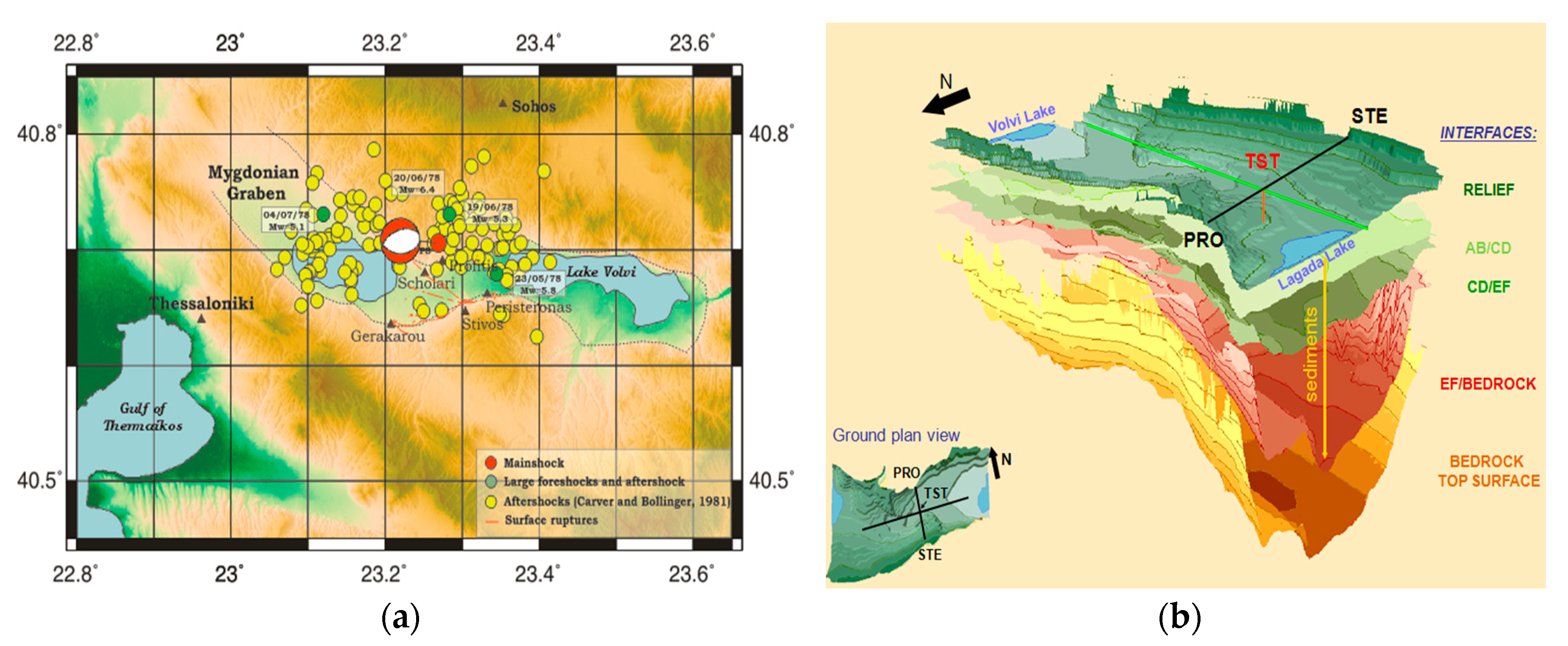
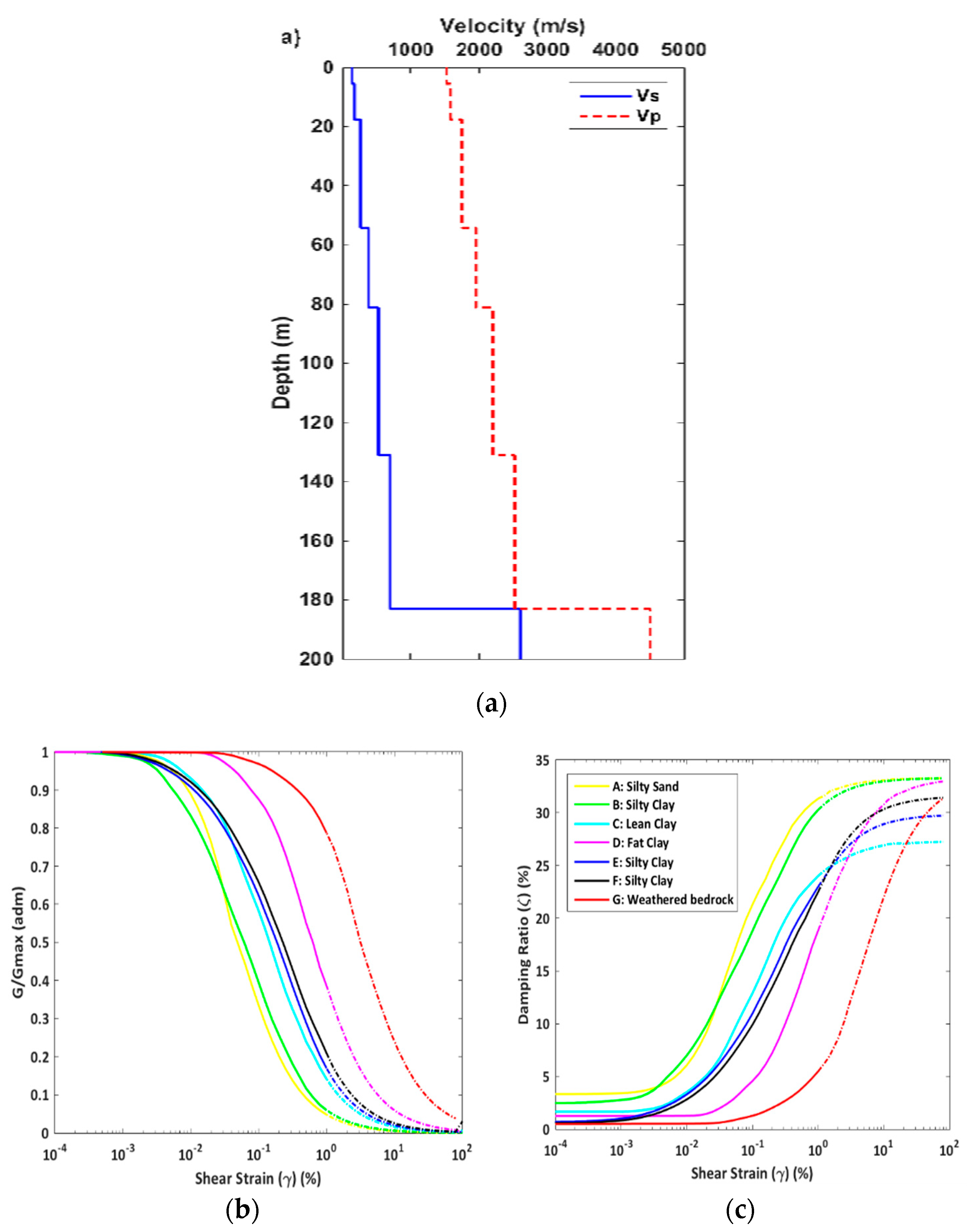
2. Study Area: The Euroseistest Site

As stated in [18], the Euroseistest site is a multidisciplinary experimental site for integrated studies in earthquake engineering, engineering seismology, seismology, and soil dynamics. It has been established thanks to European funding in Mygdonia valley, the epicentral area of the 1978, M6.4 earthquake, located about 30 km to the NE of the city of Thessaloniki in northern Greece, Figure 1a [19,20,21]. The ground motion instrumentation consists of a three-dimensional (3D) strong motion array, which has been operational for slightly more than two decades.
This site was selected as an appropriate site to perform this exercise, because of the availability of extensive geological, geotechnical, and seismological surveys. The velocity model of the Euroseistest basin has been published by several authors [22,23,24,25], varying from one-dimensional (1D) up to two-dimensional (2D) and 3D models (Figure 1b). These models were used to define the 1D soil column for the present exercise (Figure 2a and Table 1). Degradation curves are also available to characterize each soil layer, (Figure 2b,c) [26], as well as local earthquake recordings to calibrate the model in the linear (weak motion) domain. For the present exercise, in the absence of reliable measurements along the whole profile, the cohesion was assumed to be zero in all layers (C = 0 kPa). As non-zero cohesion is generally associated with non-zero plasticity index, and a shift of non-linear degradation curves towards higher strains, this zero-cohesion assumption is likely to result in a stronger impact of the NL site response, so that the present case is to be considered as an example case for a highly non-linear, deep soft site.
Several studies performed at the Euroseistest, both instrumental and numerical, have consistently shown a fundamental frequency (f0) around 0.6–0.7 Hz [23,27,28,29,30] with an average shear wave velocity over the top 30 m (VS30) of 186 m/s. The 1D simulations that are performed in this study are based on the parameters listed in Table 1, which have been shown to be consistent with the observed instrumental amplification functions, A F ( f ) , at least in the linear domain [23,27,28,29,30].

3. Methods

The methods that are followed in this work correspond to two different, fully probabilistic procedures to account for highly non-linear soil response in PSHA, a Full Probabilistic Stochastic Method (SM) that is developed for the present work, and the analytical approximation of the full convolution method (AM), as proposed by [10,11].
For both approaches, the first step consists in deriving the hazard curve for the specific bedrock properties of the considered site. As shown in Figure 2a and Table 1, this bedrock is characterized by a high S-wave velocity (2600 m/s), and is therefore much harder than “standard rock” conditions corresponding to VS30 = 800 m/s. Hence, host-to-target adjustments are required [31,32,33,34] to adjust the ground motion estimates that are provided by Ground Motion Prediction Equations (GMPEs) for the larger shear wave velocity and also possibly for the different high-frequency attenuation of the reference rock (such adjustments are commonly known as Vs-kappa effect [35]). For the sake of simplicity in the present exercise, the hazard curve has been derived with only one GMPE (Akkar et al., 2014) (AA14) [36], which is satisfactorily representative of the median hazard curve on rock obtained with seven other GMPEs deemed to be relevant for the European area (see [15]). The host-to-target (HTT) adjustments have been performed here on the basis of simple velocity adjustments calibrated on KiKnet data using the Laurendeau et al., 2107 GMPE [37], since the detailed knowledge of the site characteristics does not compensate the very poor information on the “host” characteristics of any GMPE (in particular those from European data), which results in very large uncertainty levels in classical HTT approaches [38].
For the SM approach, the next step consists in generating a synthetic earthquake catalog by sampling the earthquake recurrence model. The area source model that was developed in SHARE [18] is sampled with the Monte Carlo method to generate the earthquake catalog (OpenQuake engine, Stochastic Event Set Calculator tool [39]). The Boore (2003) Stochastic Method [40,41] is then applied to generate synthetic time histories at the bedrock site corresponding to all earthquakes in the catalog. Some specific adjustments and corrections were required to obtain ground motions compatible with the ground-motion model (AA14) used in the classical PSHA calculation. This step, which is not trivial, is described in detail in the hard rock section.
The hard rock, correctly scaled time histories are then propagated to the site surface using two different 1D non-linear site response codes. One set of time histories on soil is generated that is based on the SHAKE91 equivalent-linear (EL) code [42,43,44], while the second set was derived using the NOAH [45] fully non-linear code (NL). Both of the codes were used with the objective of incorporating somehow the code-to-code variability, which has been shown in all recent benchmarking exercises to be very important [46,47]. The final step in the SM method consists in deriving the site-specific hazard curve by simply calculating the annual rate of exceedance from the set of surface synthetic time series.
The AM approach, as proposed by [11], requires, for each frequency, f, a statistical description of the response spectrum amplification function AF ( f , S a r ) as a function of input ground motion on rock, S a r . This is done, for each used site response code, with a piecewise linear function describing the dependence of the median A F ( f ) with loading level S a r ( f ) , together with an appropriate lognormal distribution, accounting for its variability as a function of input ground motion on rock, S a r . The large number of synthetic time histories at site surface were used to derive the piecewise linear function of the AM ( A F ( f ) vs. S a r ( f ) ). Finally, the bedrock hazard curve (including host-to-target adjustments) is then convolved analytically with the simplified amplification function following [11], to obtain an estimate of the site surface hazard curve, to be compared with the SM estimate.

4. Results for Hard Rock Hazard

The site-specific soil hazard estimates at the Euroseistest using the two different fully probabilistic methods are presented below, with step-by-step explanations of the hypotheses that are considered and the obtained results.

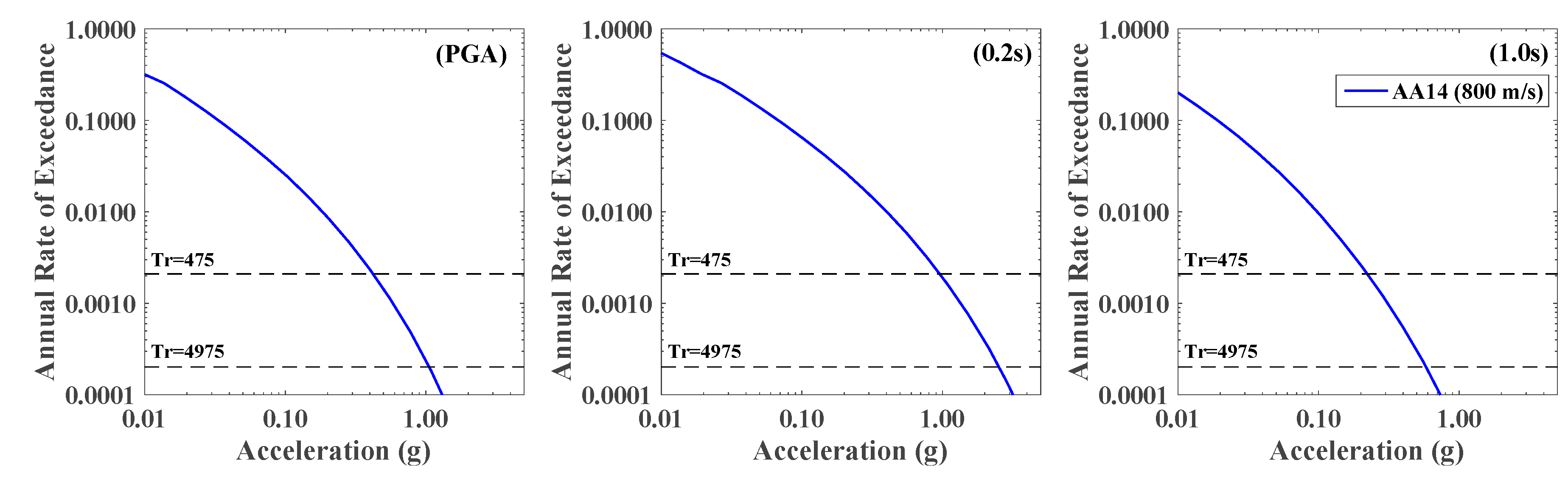
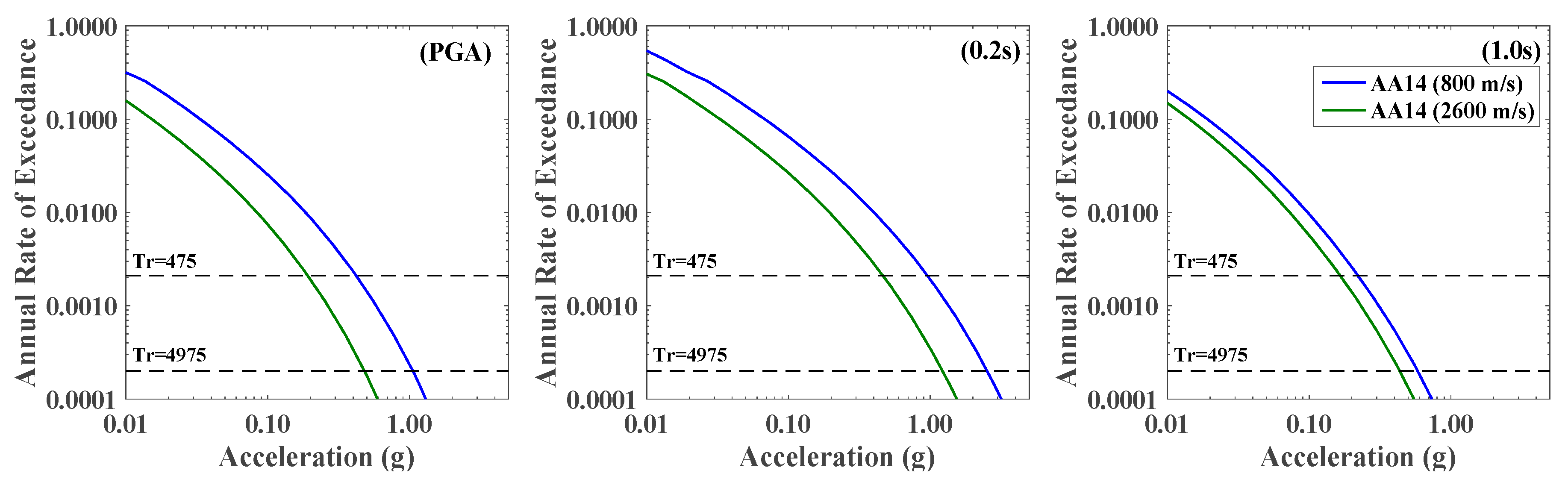
4.1. Rock Target Hazard

The first step consists in defining the target hazard on a standard rock at the Euroseistest, to be able to generate a set of consistent synthetic time histories. Following the methodology that is described in [14,15], the hazard curve calculated using the AA14 GMPE was selected as the target hazard curve for EC8 standard rock (VS30 = 800 m/s) for this exercise. Figure 3 displays the AA14 hazard curves at three different spectral periods (PGA, 0.2 s and 1.0 s, respectively) using 5% spectral damping ratio (ξ = 5%). The hazard is calculated while using the area source model that was developed in the European SHARE project [18] (xml input files available on the efher.org website) and the Openquake Engine [39,48].

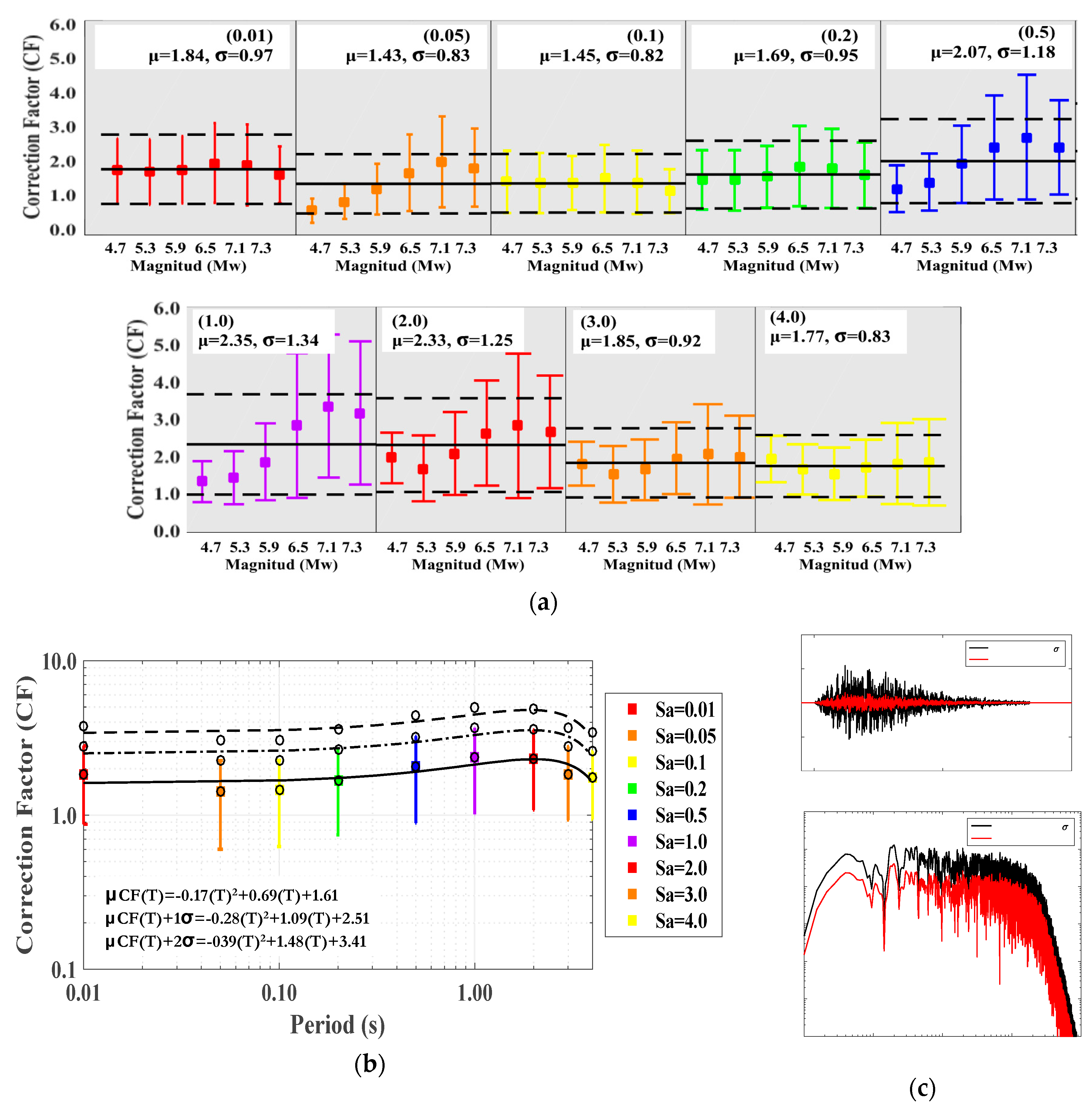
4.2. Host-to-Target Adjustments

As presented in more detail in [21,22], the bedrock beneath the Euroseistest basin (~196 m depth) has a shear wave velocity of about 2600 m/s, which is much larger than the validity range of most GMPEs. It is therefore mandatory to perform what is known in literature as “host-to-target adjustment” corrections (HTT [31,32,33,34]). As discussed in [14,15], the high level of complexity and uncertainty associated to the current HTT adjustments procedures [16,37,49,50,51], have motivated us to use here another, simpler, straightforward way to account for rock to hard rock correction for probabilistic seismic hazard purposes.
This simpler approach is based on the work by Laurendeau et al., 2017 (LA17) [37], who proposed a new rock GMPE that is valid for surface velocities ranging from 500 m/s to 3000 m/s and derived on the basis of the Japanese KiK-net dataset [52]. This GMPE presents the advantage to rely only on the value of rock velocity, without requiring the κ0 values either for the host region or for the target site, and therefore avoiding the associated uncertainties. The adjustments are thus performed on the basis on one single proxy for rock, as it is usually done for all soil deposits. It may account for the variability of some other mechanical characteristics (such as κ0, or the fundamental frequency f0), but only through their potential correlations with VS30. We consider, as discussed in [37,38], that such an approach is as reliable as the conventional HTT approach due to the huge uncertainties and possible bias linked with the measurement of the physical parameter κ0. It provides rather robust predictions of rock motion whatever the approach used for their derivation: deconvolution of surface recordings to outcropping bedrock with the known 1D profile, or the correction of down-hole recordings, see [37] for the corresponding discussion.
The LA17 GMPE is based on a combined dataset including surface recordings from stiff sites and hard rock motion estimated through deconvolution of the same recordings by the corresponding 1D linear site response. The site term in the proposed (simple) GMPE equation is given by a simple dependence on rock S-wave velocity value VS30 in the form S 1   ( T ) .   l n ( V S 30 / 1000 ) , where S 1 is tuned from actual recordings for each spectral oscillator period ( T ). The HTT adjustment factor can thus be computed, as follows in Equation (1):
  H T T   A d j u t m e n t   F a c t o r s ( T ) = H a r d   R o c k   H C   ( V s = 2600   m / s ) S t a n d a r d   R o c k   H C   ( V s = 800   m / s ) = S 1 ( T ) . l n   ( 2600 / 800 )  
Since the site terms in LA17, for such hard and standard rock, do not include any non-linearity, the resulting HTT adjustment factors are ground-motion independent, and thus return period (Tr) independent. The correction procedure consists simply in computing the hazard curves for standard rock (VS30 = 800 m/s) using AA14 GMPE, and then correcting it with the so defined, frequency-dependent LA17 HTT factor. The values listed in Table 2 indicate that hard rock motion is systematically smaller than the standard rock motion at all of the spectral periods, with larger reduction factors at short periods. Of course, these corrections are, in principle, only valid for Japanese rock sites, but on the other hand most of HTT methods are implicitly using, in practice, typical United States-California (US-California) velocity rock profiles at least for the host side. There is no obvious reason why such US profiles would be more acceptable for Europe than Japanese results. Ultimately, the hard-rock hazard curve is then derived by simply scaling the AA14 hazard curve with the HTT adjustments factors for each period (Figure 4).
One might wonder why scaling AA14 curve instead of using directly LA17 in the calculations. The main reason was that AA14 (VS30 = 800 m/s) provides a good approximation to the median hazard estimate at the Euroseistest on standard rock from seven explored GMPES [15], while the estimates with LA17 (VS30 = 800 m/s) is located outside the uncertainty range of the same selected representative GMPEs. This is probably due to the very simple functional form that is used in LA17, and to the fact that it was elaborated only from Japanese data. Its main interest however is to provide a rock adjustment factor calibrated on actual data from a large number of rock and hard rock sites, without any assumptions regarding non-measured parameters, such as κ0. Once the approach that is proposed here and initially based in LA17 is tested on other data sets, the corresponding results can be used to provide alternative scaling factors between hard rock and standard rock. Note, however, that this modulation approach through another kind of GMPE is exactly similar to what has been proposed in [16], where stochastic simulations are used for the VS-κ corrections without being used as GMPEs.

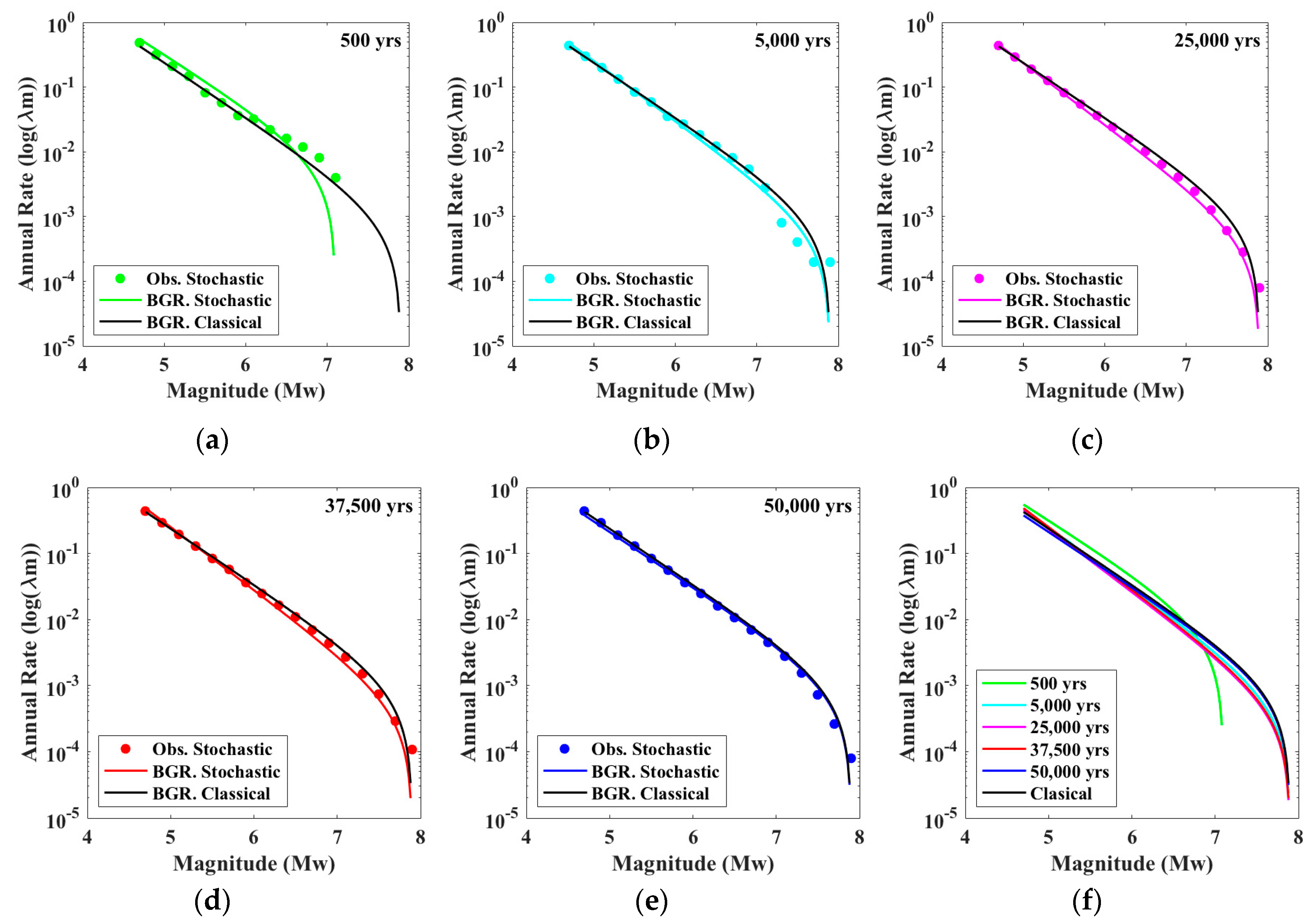
4.3. Synthetic Earthquake Catalog

Once defined the target hazard on hard rock, we proceed to generate a long enough seismic catalog to build synthetic hazard curves both on rock and soil at the selected Euroseistest site. The earthquake catalog is obtained by sampling the area source model of SHARE. To handle a reasonable amount of events, only the sources that are contributing to the hazard must be sampled. To identify which area sources contribute to the hazard at the Euroseistest site, the individual contributions from the crustal sources in the neighborhood of the site were calculated. The individual hazard curves corresponding to each source were compared to the total hazard curve using all sources, showing that the area source enclosing the Euroseistest site (GRAS390) fully controls the hazard at all of the considered periods, so that we can neglect the other sources in our calculations.
The stochastic earthquake catalog was generated by sampling the magnitude-frequency distribution (truncated Gutenberg-Richter model) of the area source zone, and earthquakes are distributed homogeneously within the area source zone. For this purpose, we use the Stochastic Event Set Calculator tool from the Openquake Engine [39,48]. The generated catalog must be long enough to estimate correctly the hazard for the return period of interest, 5000 years (equivalent to a probability of exceedance of 1.0% in 50 years). The length of the catalog is obviously a key issue when calculating seismic hazard with the Monte Carlo technique.
To identify which minimum length is required, a sensitivity analysis is led consisting in comparing the different magnitude-frequency distribution curves and hazard curves that were obtained with different catalog lengths. Figure 5 displays the magnitude-frequency distribution curves built using increasing catalog lengths (500, 5000, 25,000, 35,500, 50,000 years), when compared to the original SHARE model (black solid line). For short catalog lengths (here 500 years), the recurrence model is not correctly sampled in the upper magnitude range. The catalog length is too short with respect to the recurrence times of large events. When considering longer catalog lengths (from 5000 years on), the full magnitude range is sampled. However, the correct annual rates for the upper magnitude range are obtained with a reasonable error (~5%) only for very long earthquake catalog lengths (larger or equal to 50,000 years). Most important is that the magnitude range contributing to the hazard at the return periods of interest are correctly sampled.
Figure 6a display the stochastic hazards curves on rock obtained from the five catalogs with increasing lengths, as well as the hazard curve calculated with the classical PSHA calculation (using AA14 ground-motion model). Figure 6b illustrates the ratio between the PGAs relying on the Monte Carlo method and the PGAs relying on the classical approach, interpolated for different annual rates. Based on these results, we decide to use a 50,000 years earthquake catalog to estimate the hazard, since the difference between PGAs is lower than 5% for all of the annual rates down to 10−4 (or return periods up to 10,000 years). The final selected catalog of 5000 years consists of ~21,800 events ranging from the minimum considered magnitude Mw = 4.5 to the maximum magnitude Mw = 7.8, with a distance range (Joyner and Boore) from 0 to 150 km and a depth range from 0 to 30 km.

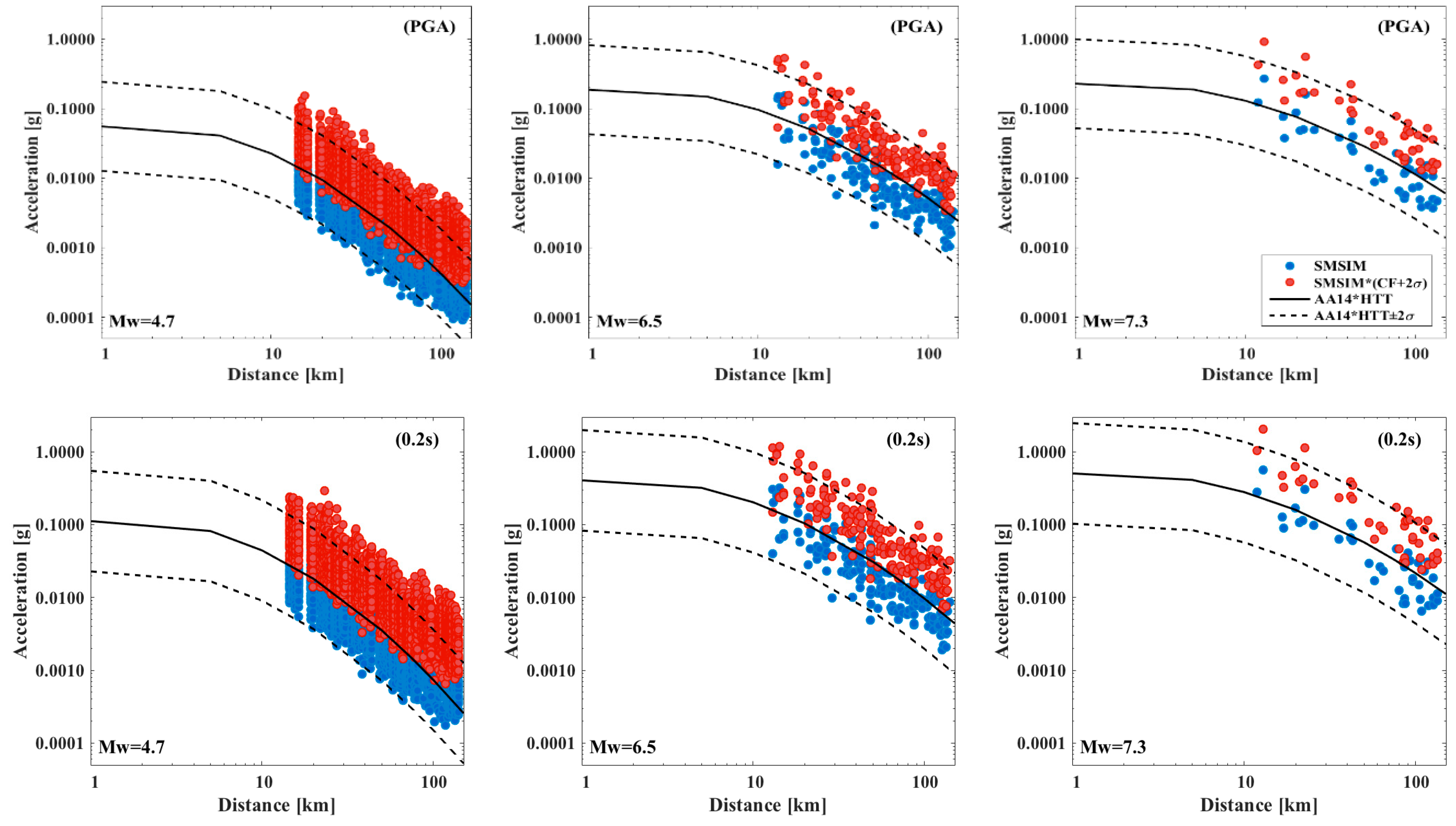
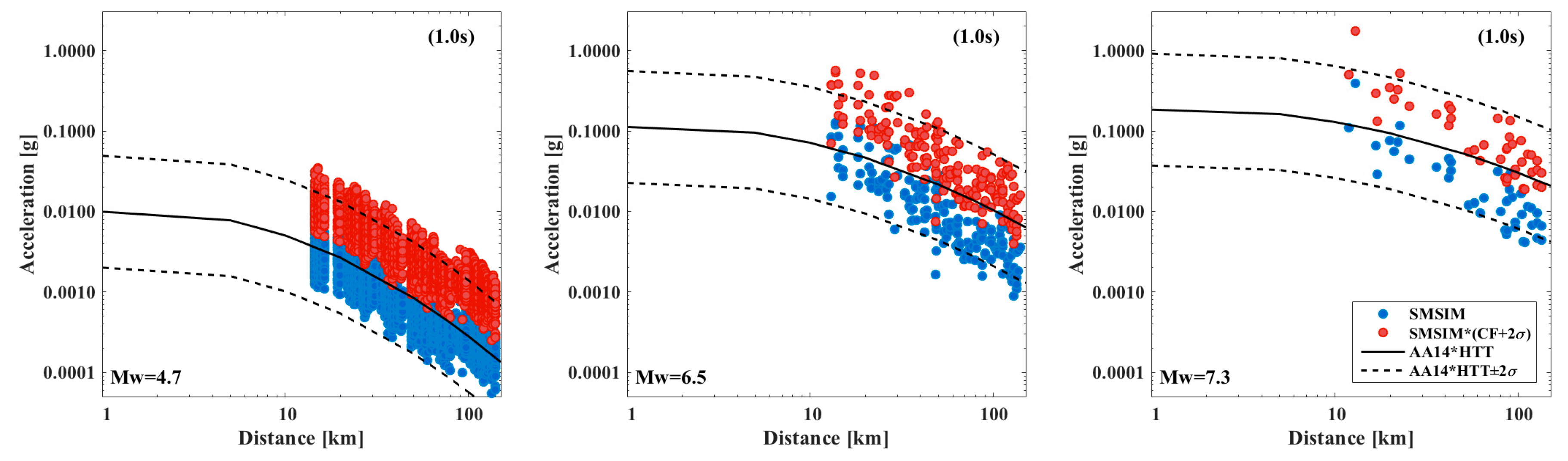
4.4. Synthetic Time Histories on Rock

Now, we can proceed to generate synthetic time histories on hard rock. We propose to define the input motions combining a simple approach to generate synthetic time histories with the AA14 GMPE. An arbitrary seismological model is used to generate the waveforms that are then scaled to match the target accelerations, using a continuous function. We consider that it is reasonable: (1) to define the input motions using the European AA14 GMPE and (2) to generate synthetic time histories that are compatible to the selected GMPE on the basis of a simple, point source seismological model with plausible but arbitrary source and path parameters, providing waveforms that are later scaled using a continuous function to match the target accelerations at different spectral periods.
We use the well-known stochastic method that was proposed by D. Boore [40] for the generation of ground-motion time histories, and its corresponding Fortran code SMSIM [41], which is freely provided by the author on his website. Any other suitable method to generate synthetic time histories could be used. This step is one of the most time consuming of the entire process, since the length of the earthquake catalog implies a very large number (~21,800) of events and thus the generation of numerous time histories at the site. The main input parameters are [40]: the source characteristics (seismic moment M0 and stress drop Δσ or corner frequency fc), the path terms with geometrical spreading G(R), anelastic attenuation Q(f), and duration terms Tgm(f) related to hypocentral distance Dhyp, the frequency f , and the site terms including the crustal amplification factor CAF(f) derived from the site velocity profile VS(z), together with the site specific shallow attenuation factor characterized by the κ0 value. When considering the published, locally available data at the Euroseistest site, the Boore stochastic method has been applied with the crustal velocity structure detailed in [26], a κ0 value of 0.024 s [53], and a lognormal distribution of the stress drop with a median value of 30 bars and standard deviation of 0.68 (natural log). The ground-motion duration (Tgm) used here corresponds to the sum of the source duration, which is related to the inverse of the corner frequency (1/fc) and a path-dependent duration (0.05 R follows [54] model).
We calculate the hazard curves on rock based on the synthetic time histories generated using SMSIM (Figure 7, PGA, 0.2 s and 1.0 s). The annual rates of the generated time histories are significantly lower than the rates of the target hard-rock hazard curve relying on AA14 GMPE (green curve on Figure 7). Such a discrepancy is related to the lack of consistency between the theoretical stochastic approach (source, path, and site term) and the empirical AA14 GMPE. A correction should thus be applied to the results of the stochastic simulation, which can be done in several possible ways. The first way consists in tuning the SMSIM ground-motion model, by performing a sensitivity analysis on the input parameters (geometrical spreading term, crustal attenuation, Δσ, κo) until a hazard curve close to the target hazard curve is obtained. We tried this approach on a trial-and-error basis, but we found it to be very time-consuming and rather inefficient in obtaining time histories simultaneously compatible at all spectral periods. Actually, such an approach would require a full inversion of the “free” parameters mentioned above, as performed recently, for instance by [55]. Hence, we opt for a much faster, easier, and entirely pragmatic scaling technique, as described below.
First we calculated the median accelerations predicted by AA14 (VS30 = 800 m/s), for the magnitude set Mw = [4.7, 5.3, 5.9, 6.5, 7.1, 7.3] and distances Dhyp = [1, 5, 10, 20, 50, 75, 100, 150] km at a series of spectral periods T = [0.01, 0.05, 0.2, 0.2, 0.5, 1.0, 2.0, 3.0, 4.0] s. These AA14 predictions were corrected while using the site term of the LA17 GMPE to derive the expected motion for a hard rock with Vs = 2600 m/s (see HTT, Section 4.2). Then, for each event (Mw, Dhyp), we calculate the ratios between the synthetic spectral acceleration and the corrected AA14 acceleration (VS30 = 2600 m/s). The ratios that were obtained for different spectral periods are displayed in Figure 8a. The error bar represents the median ± one standard deviation calculated over all the ratios available for a given magnitude. The variability comes from the inconsistency between the distance term in the AA14 GMPE and its equivalent contribution in the SMSIM approach (i.e., the combination of the geometrical spreading term and the crustal/site attenuation terms).
The horizontal black lines in Figure 8a represent the average correction factors when all magnitudes and distances are considered and the associated standard deviation (dashed lines). These values are displayed in Figure 8b as a function of the spectral period, showing that the largest correction corresponds to rather long periods (around 2.0 s), suggesting that part of this discrepancy could be due to the fact that only point sources were considered. Indeed, the correction factors in Figure 8a increase with magnitude, which suggests that the use of a code considering extended source should be preferred. Figure 8b also displays the values of the median correction factor + one and two standard deviations, and their interpolation from period to period to derive a continuous, period-dependent average correction factor, required to scale the generated stochastic time histories to match the target hazard at all spectral periods.
The next step consisted in scaling the ~21,800 stochastic time histories by applying the continuous correction factors (Figure 8b) derived in the response spectra domain to each one of the time histories in the Fourier domain, and posteriorly retrieving the new scaled time histories by inverse Fourier transform, as shown in Figure 8c. After the scaling process is performed, we calculate the new hazard curves based on the scaled accelerograms. Figure 9a shows the newly scaled hazard curve, this time being closer to the target hazard curve (AA14 2600 m/s) than the original one, but still with lower annual rates. We applied the same correction procedure using the median + one standard deviation (CF+1σ) and median + two standard deviations (CF+2σ) correction factors. The resulting hazard curves are displayed in Figure 9b,c.
The ratios between the target AA14 accelerations (VS30 = 2600 m/s) and the scaled stochastic accelerations, interpolated for a series of annual exceedance rates, are shown in Figure 10. The best agreement is obtained by applying the (CF+2σ) scaling factor; the resulting ratio is close to 1.0 for most annual rates of exceedance (and especially the smallest) at the three displayed spectral periods. It is important to mention that the (CF+2σ) correction factor is a pragmatic non-physical parameter that we used to scale the accelerograms in order to fit a certain target hazard level.
Figure 11 displays the synthetic mean spectral acceleration values before and after the scaling process and is compared to Akkar et al., 2013 [36] scaled while using the HTT factors (Figure 11). This plot is shown for three different spectral periods (PGA, 0.2 s, 1.0 s) and for events of Mw = [4.7, 6.5, 7.5]. Events in the catalog were generated for different hypocentral distances (Dhyp) and a scaling factor at +2σ was applied to generate compatible hazard curves as explained in the previous step. As mentioned before, this correction is only a pragmatic way of scaling accelerograms and it does not rely on a physics-based scaling strategy. Nonetheless, it does provide a very satisfactory fit between the stochastic hazard curves and the target hazard curves at all spectral periods, and it upholds the original variability of the accelerograms. Future applications should improve this step to find a physics-based optimal fitting procedure (such as higher, possibly magnitude-dependent, stress drops, frequency-dependent geometrical spreading, and crustal quality factor).

5. Results for Soft Soil Hazard

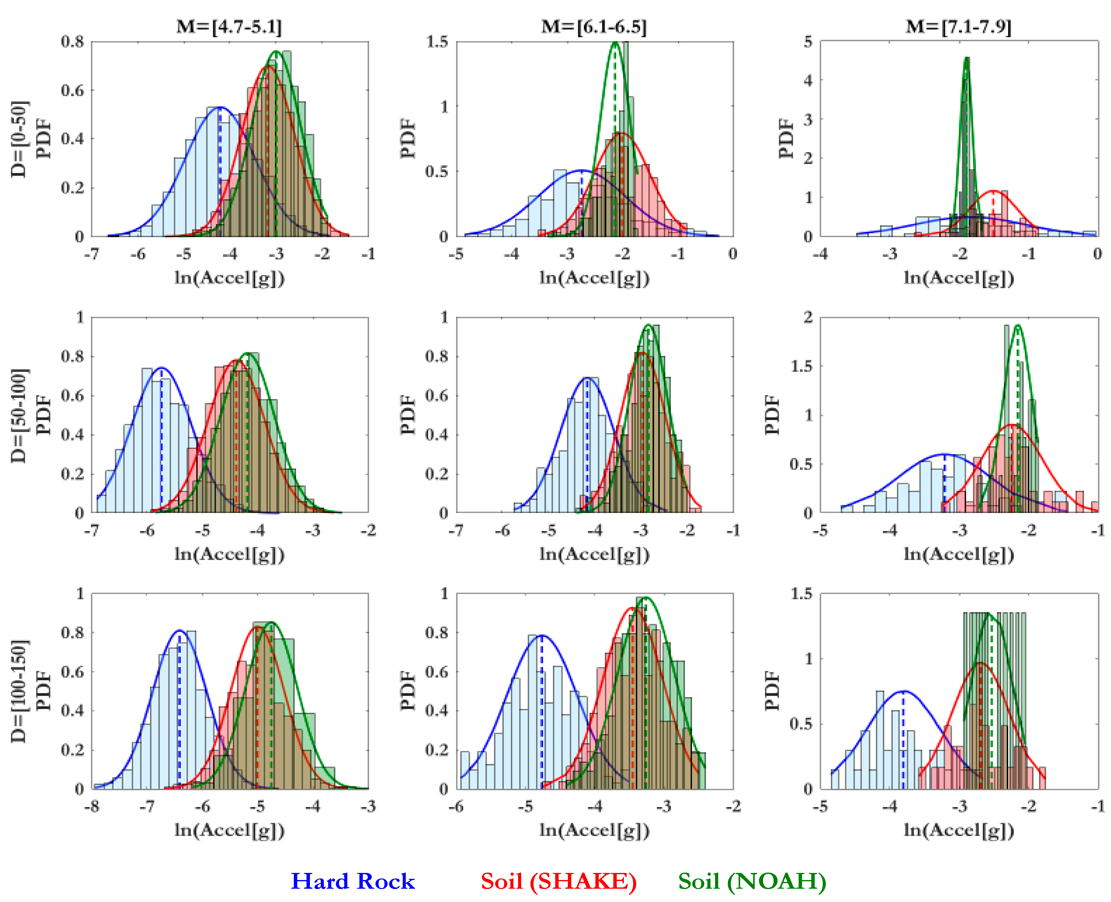
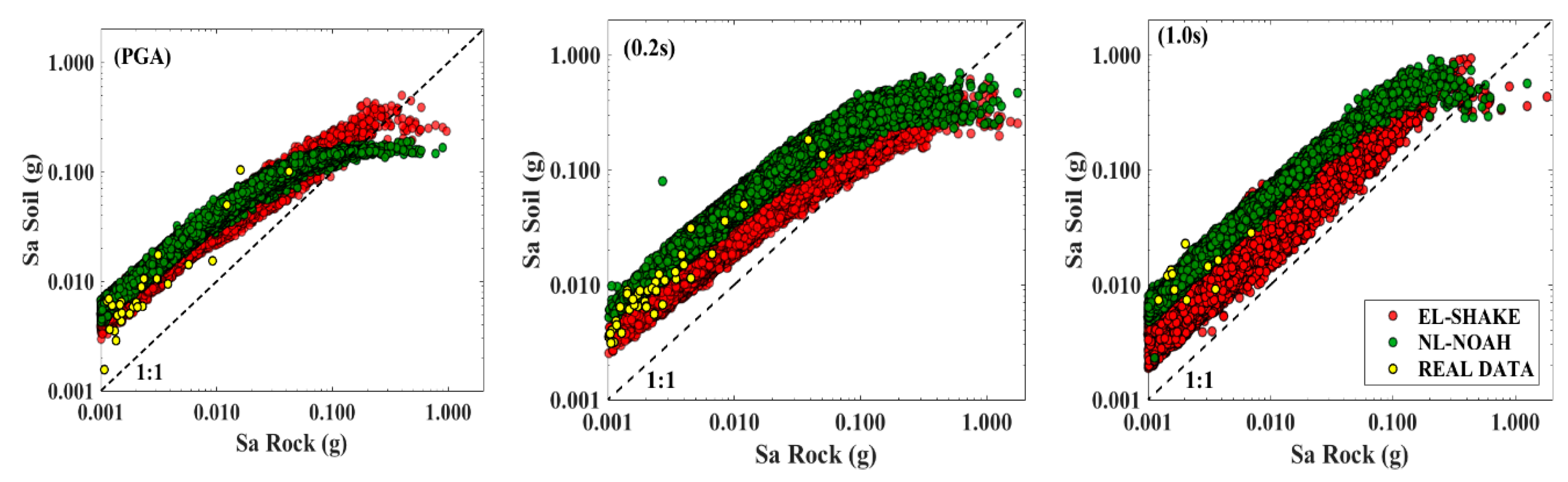
5.1. Synthetic Time Histories on Soil

Based on the (CF+2σ) scaled synthetic time histories on hard rock, we can now generate the corresponding time histories on soil by performing a 1D equivalent-linear (EL, SHAKE91 [42,43,44]) and 1D non-linear (NL, NOAH [45]) site response analyses.
The soil profile (Table 1) and the degradation curves for all layers (Figure 2b,c) were used to perform the 1D site response calculations. SHAKE91 requires only degradation curves, while NOAH requires the maximum stresses, related to the cohesion, friction angle φ, and the coefficient of earth at rest K0. For the present exercise, the cohesion was assumed to be zero in all layers since no sufficient information was available being related to this parameter, especially at large depths. It is important to highlight that the (CF+2σ) scaled synthetic time histories on hard rock are representative of the AA14 (VS30 = 2600 m/s) ground motion predictions for outcropping conditions, and this should be specified inside the site response input files in order to appropriately remove the free field surface effect (about a factor of ~2.0).

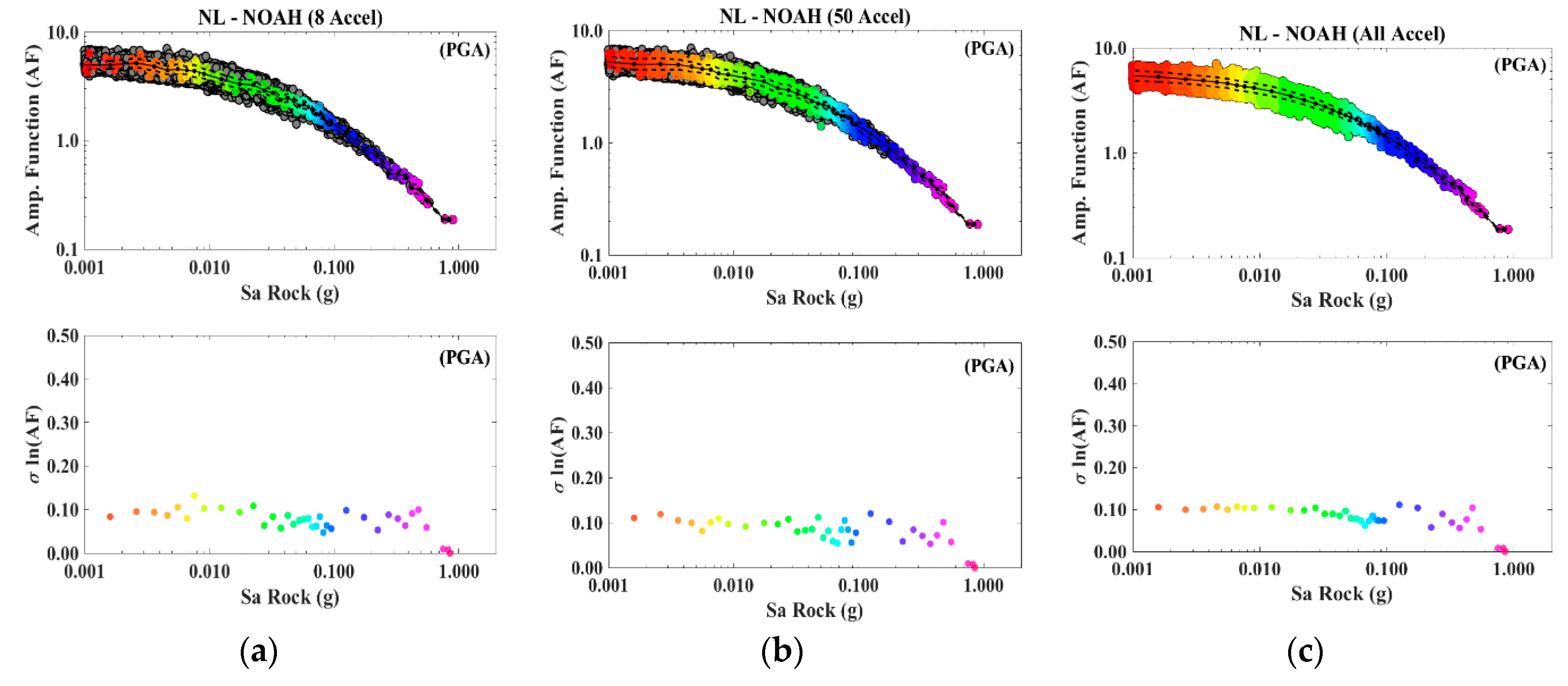
5.1.1. Focus on Nonlinear Ground Motion Saturation

An interesting way to analyze the surface synthetics is to compare the spectral acceleration on soil, with respect to the corresponding input ground motion on rock. Figure 12a shows the results at three spectral periods (PGA, 0.2 s and 1.0 s) for the SHAKE91 computations and Figure 12b for the NOAH computations.
In both cases, the soil presents significant nonlinear behavior, even at weak/intermediate motion levels (0.01 g–0.1 g), and de-amplification is observed on soil with respect to the rock motion at ground motion levels around (0.1 g–0.3 g). Moreover, a saturation level of the acceleration is always reached in both soil cases (SHAKE91 and NOAH) and at all spectral periods. The point where the saturation limit is reached depends strongly on the spectral period (at least for this example), and less on the propagation code that is used for the site response analysis. The saturation limit appears faster at high frequency than at low frequency for both codes. These results also indicate a larger variability of the data for a given rock input level when using SHAKE91 when compared to the NOAH results. Using SHAKE91, the dispersion of calculated accelerations increases with the spectral period (this is not the case using NOAH).

5.1.2. Ground Motion Variability

It is also of interest to better comprehend what happens with the ground motion variability after performing the 1D site response analysis with the two selected codes. For this purpose, we compared the probability density function (PDF) of the ground motion acceleration (PGA) on hard rock at depth with respect to the PDF on soil, for different magnitude and distance ranges (Figure 13).
A systematic amplification of the median ground motion at soil surface (SHAKE91 and NOAH) with respect to hard rock at depth is observed for small magnitudes M = [4.7–5.1] and all distances (Figure 13a). Non-linearity of the soil is not observed, indicating mostly linear behavior of the soil. Similarly, Figure 13b shows the ground motion variability at the intermediate magnitude range Mw = [6.1–6.5] at different distances (Dhyp) ranges. Amplification of the ground motion with respect to hard rock at depth is again observed. However, this time a clear saturation of the ground motion occurs at all distances due to the nonlinear effect of the soil (PDF truncated on the strong motion side, with more pronounced effect at short distances). This saturation is stronger using NOAH rather than SHAKE91, since NOAH is a fully nonlinear code. However, part of the difference can be also explained by intrinsic code differences and different degradation curves definition. At short distances, a smaller amplification and even deamplification on soil with respect to rock is observed.
Finally, for large magnitudes Mw = [7.1–7.9], a strong saturation of ground motion can be observed (Figure 13c), especially when using NOAH. It is also interesting to notice that the variability of the soil ground motion, σ S a s ( f ) , is smaller than the variability of the hard rock ground motion, σ S a r ( f ) . [2] also discussed this phenomenon, which has also been observed from real recordings on rock and soil conditions (see [56,57,58,59]).

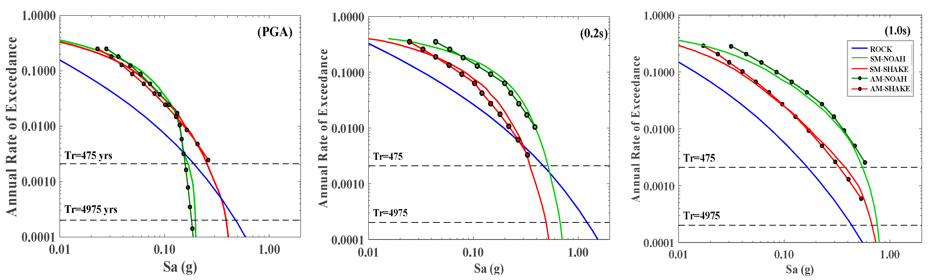
5.2. Full Probabilistic Stochastic Method (SM)

What we call here the full probabilistic stochastic method is nothing else than the hazard curve built from stochastic time histories (~21,800 accelerograms), corresponding to the strong-motion history at the site during 50,000 years.
To build the stochastic hazard curves, we calculate the annual rate of exceedance, λ ( x X ) , of a series of ground motion levels (X), for a given spectral period (T), by counting the number of occurrences of ground-motions (N) exceeding a certain ground motion level x, as follows:
  λ T ( x X ) = N   ( x X ) Catalogue   time   length  

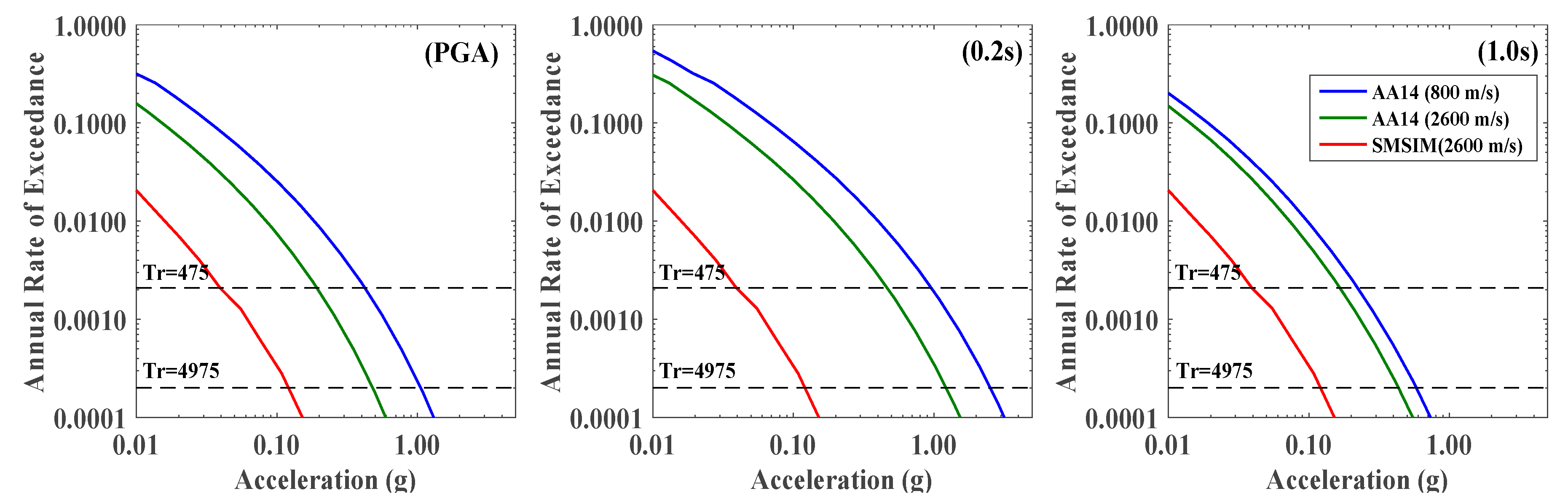
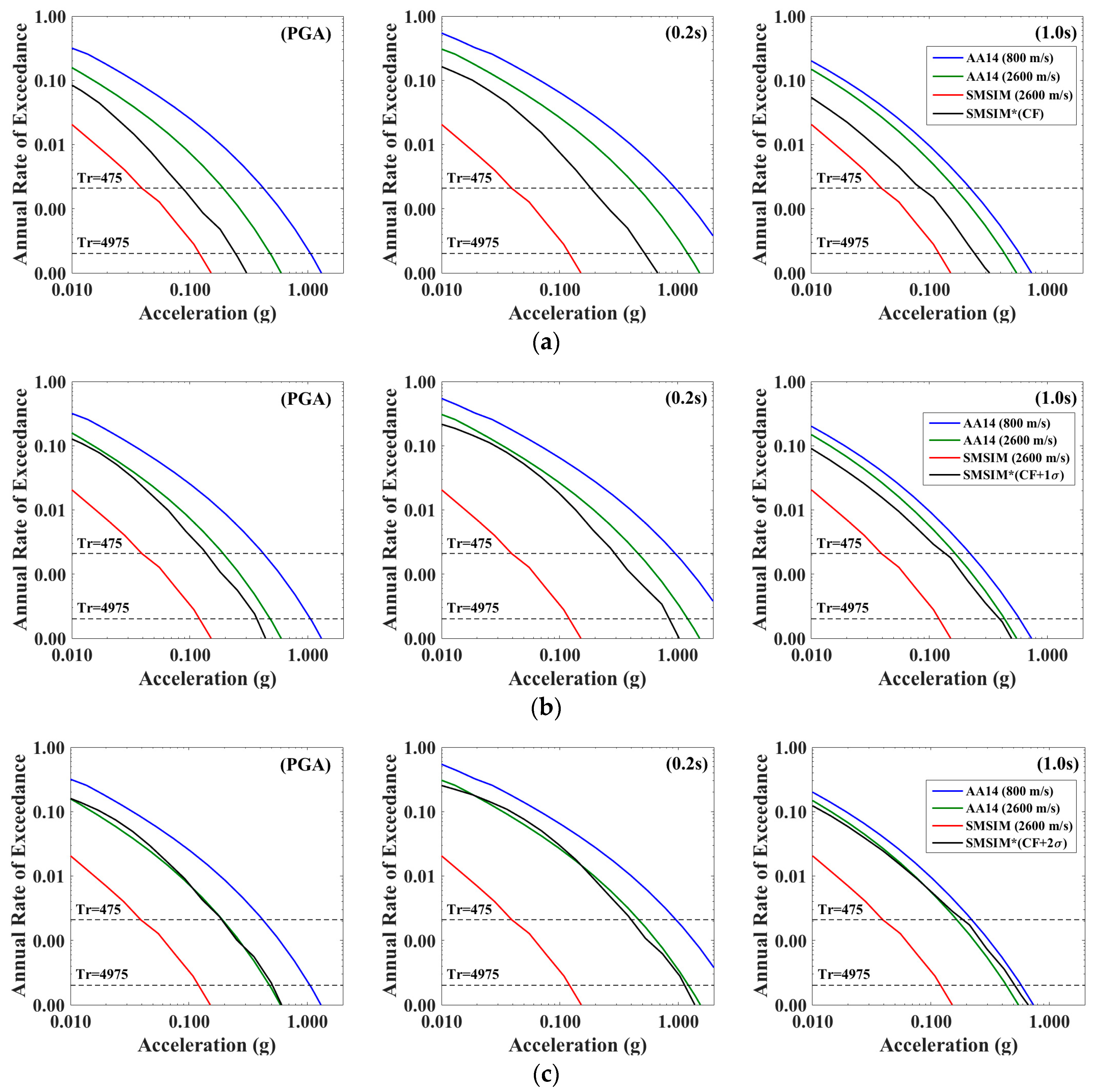
5.2.1. SM Results for Hard Rock

The stochastic hazard curve on hard rock, H C ( f ) , is thus built from the annual rate of exceedance of the scaled synthetic time histories set, as expressed in Equation (2), for three different spectral periods (PGA, 0.2 s and 1.0 s), Figure 14 (black).

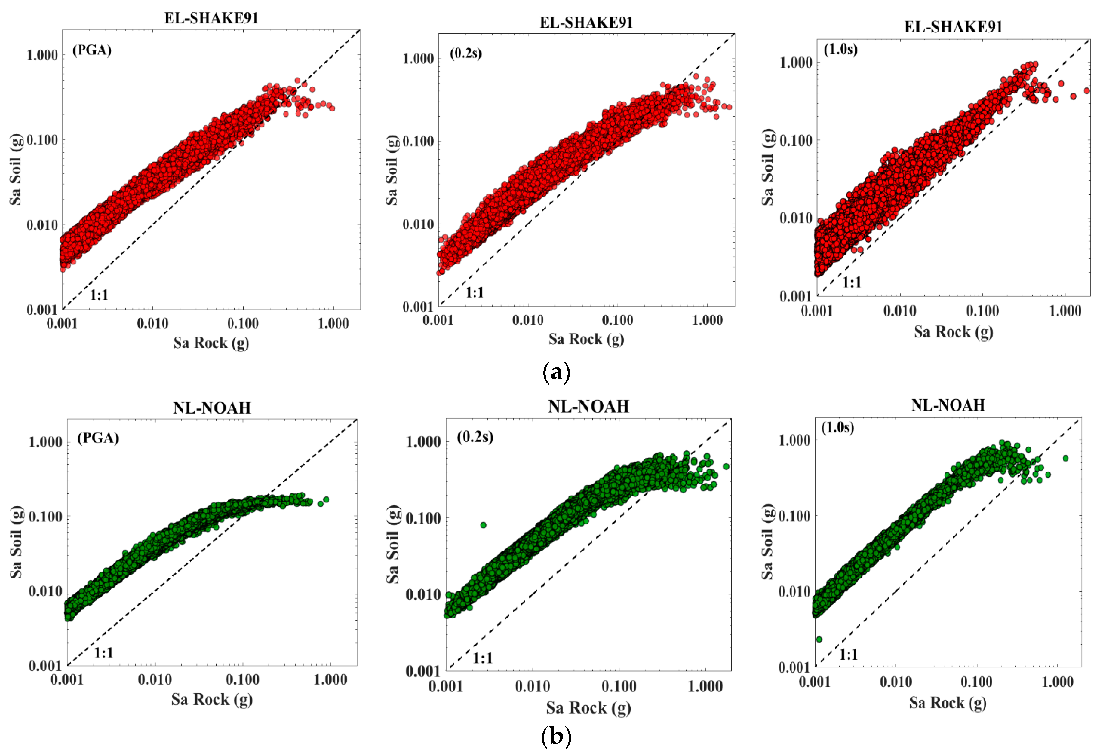
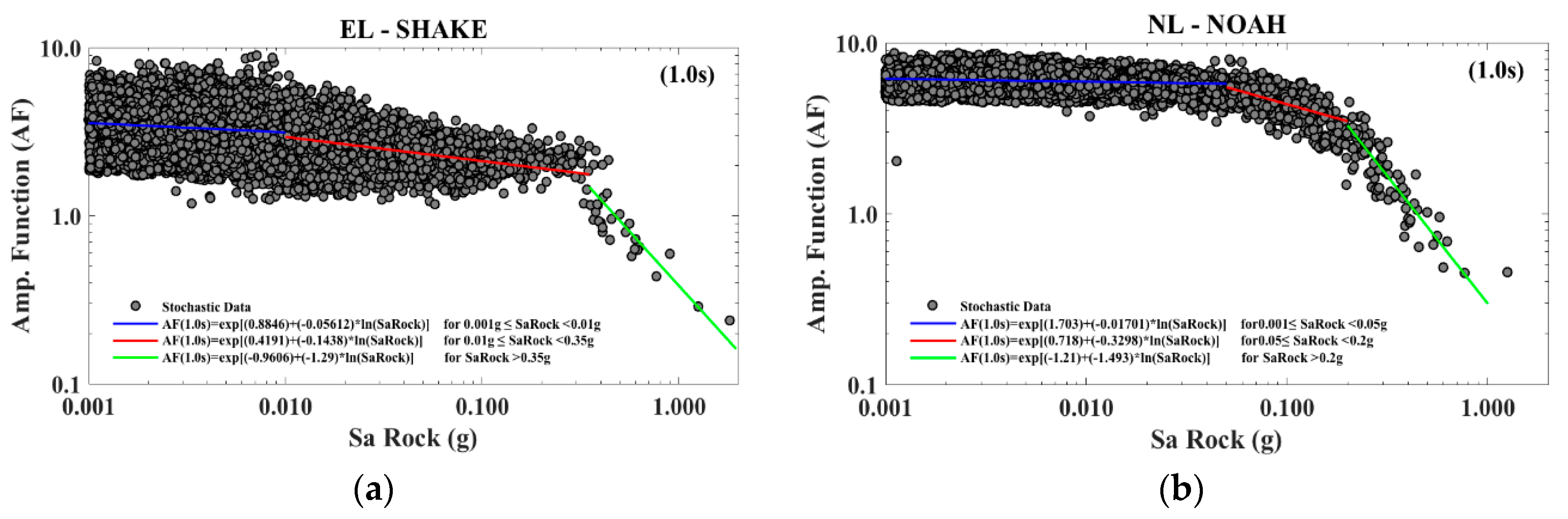
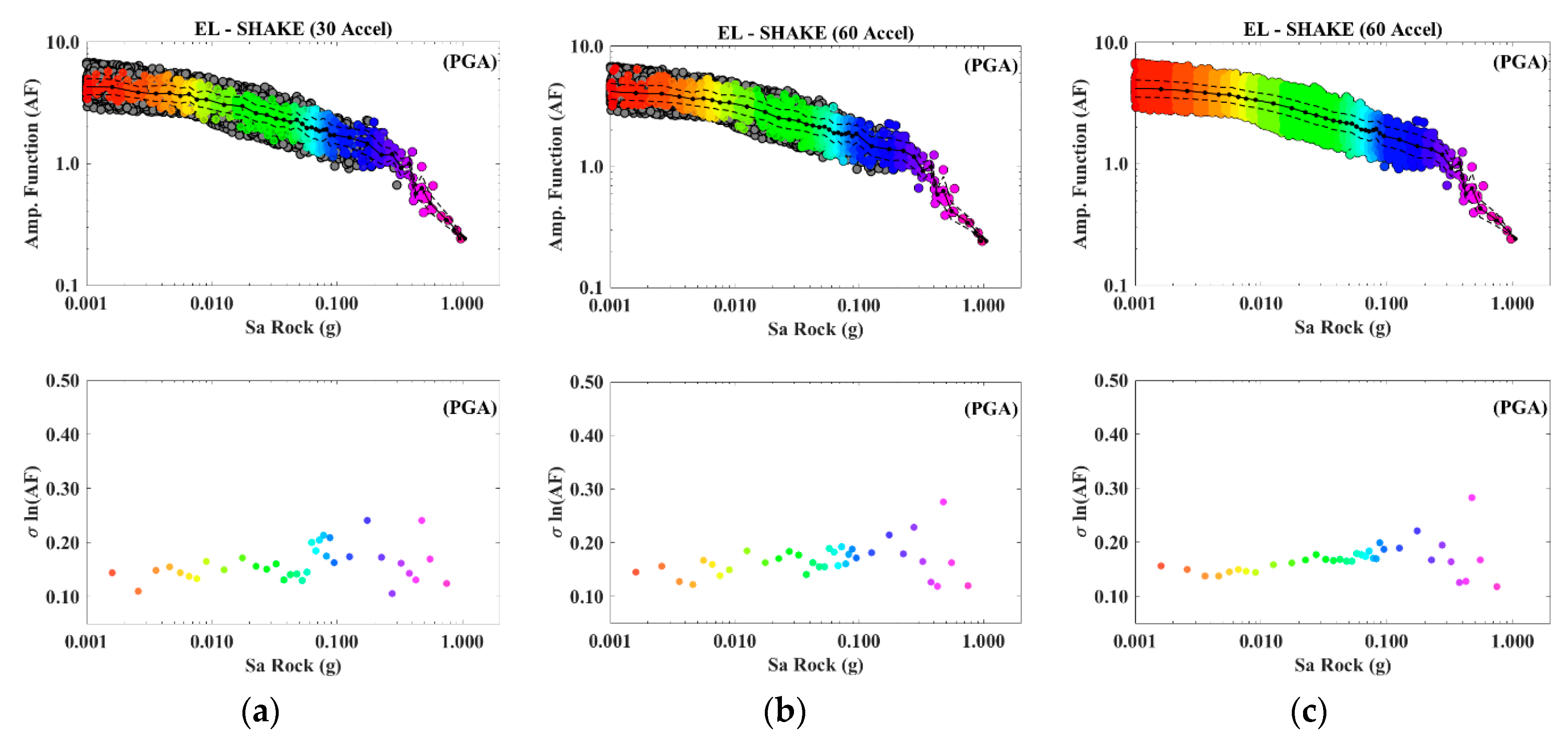
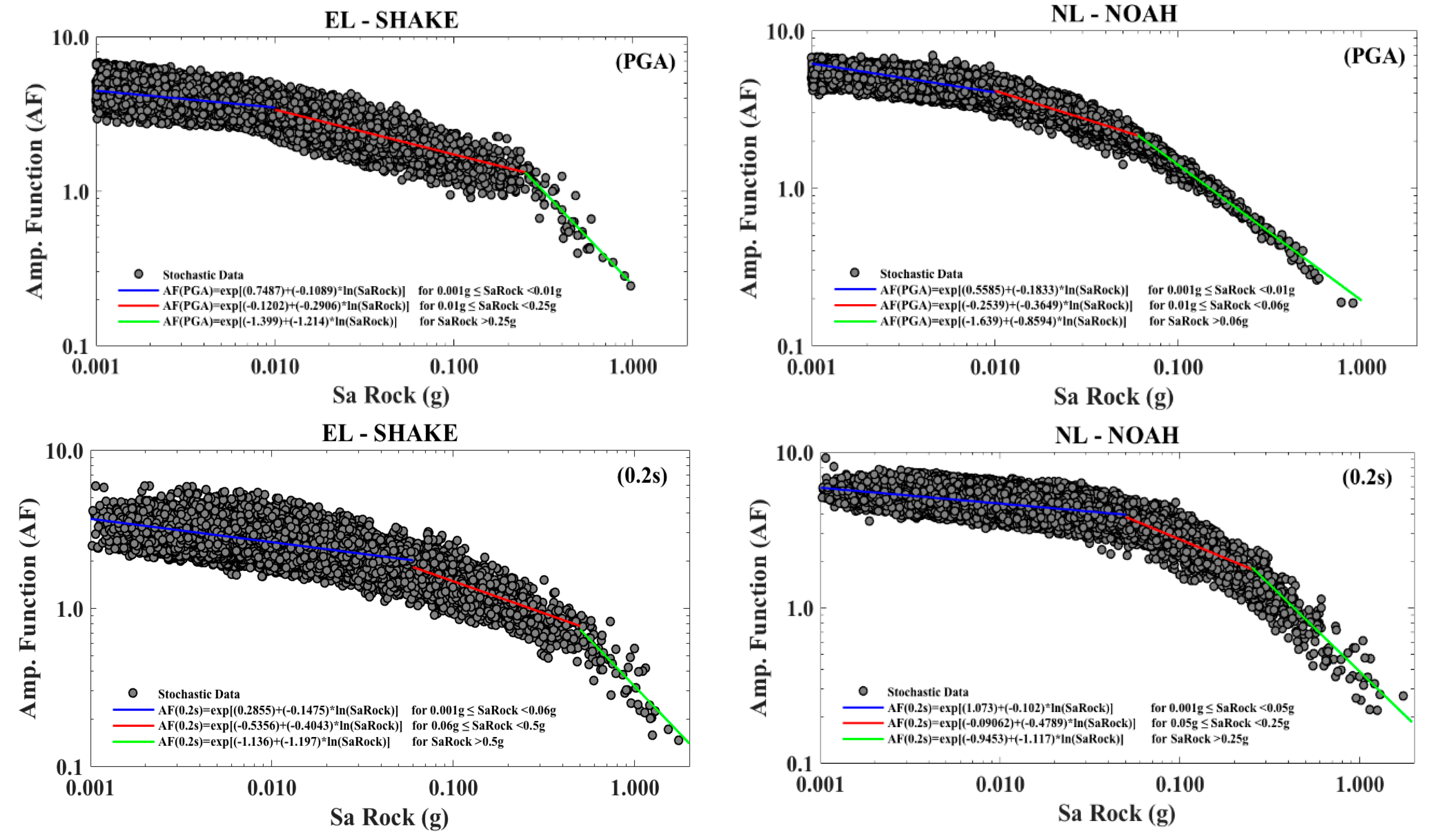
5.2.2. SM Results for Soft Soil Using SHAKE91

Similarly, we calculate the hazard curves on soil at the site for different spectral periods, while using the synthetic time histories on soil that was obtained with the SHAKE91 equivalent-linear site response analysis code. The results displayed in Figure 14 exhibit two characteristic features when compared to their rock equivalent. For all spectral periods, the soil hazard curves exhibit a much stronger convexity than for the rock hazard curves: this is related to the non-linear behavior of soil, which saturates the ground motion for the upper acceleration range at long return periods. This is also true for the largest spectral period considered here (1.0 s), because it corresponds to a shorter period than the site fundamental period (around ~1.5 s), and therefore it is affected by the non-linear behavior over the whole soil column.

5.2.3. SM Results for Soft Soil Using NOAH

Lastly, we calculate the hazard curves on soil at the site based on the synthetics that were obtained with NOAH (see Section 5.1). Results displayed in Figure 14, exhibit the same overall features than the SHAKE91 results: a pronounced convexity related with the existence of an upper bound for the surface ground motion due to the non-linear behavior. As the saturation is better accounted for in fully NL codes than in equivalent-linear approaches, the hazard curve that was predicted using NOAH is saturated at acceleration levels lower than in the SHAKE91 case.

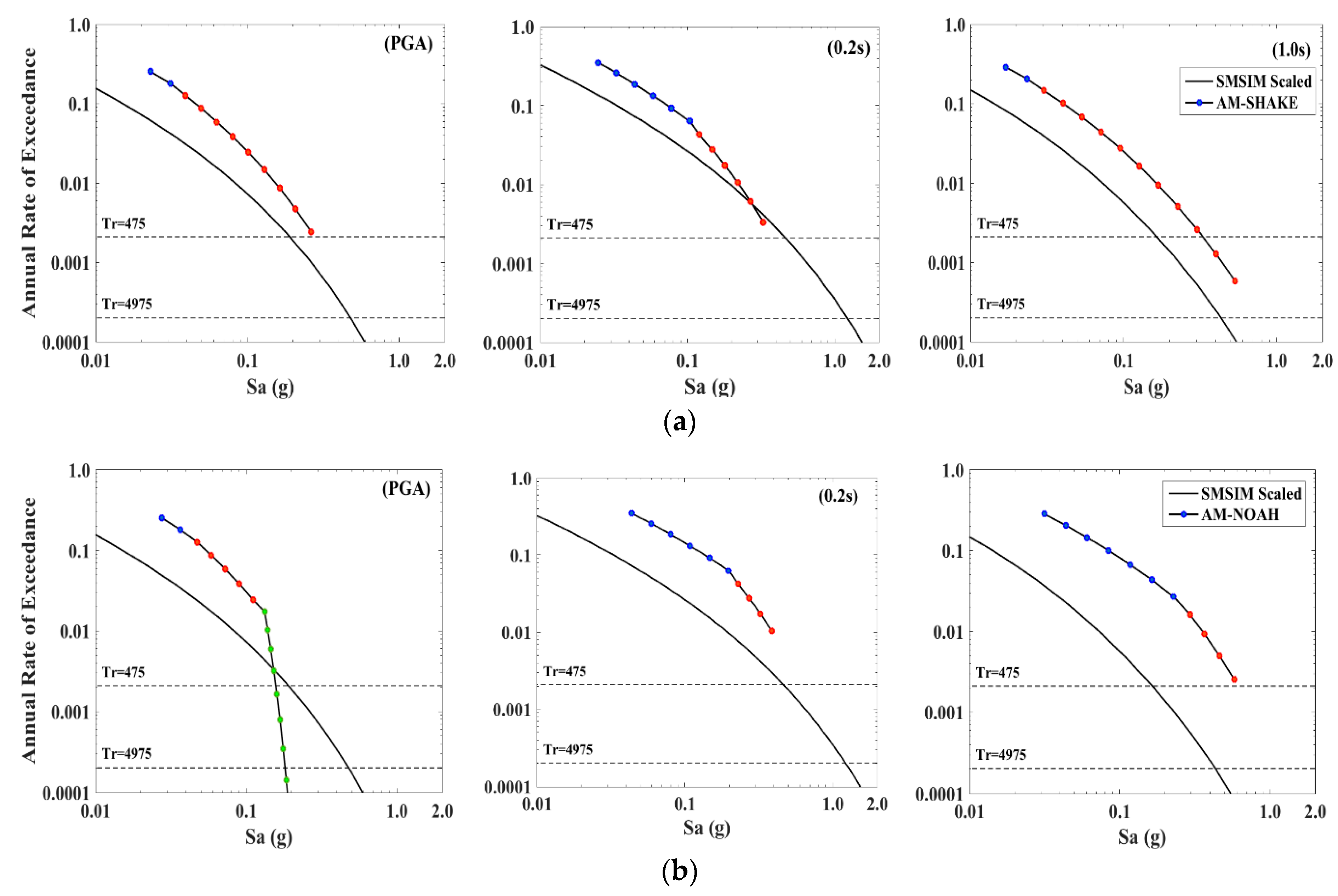
5.3. Analytical Approximation of the Full Convolution Method (AM)
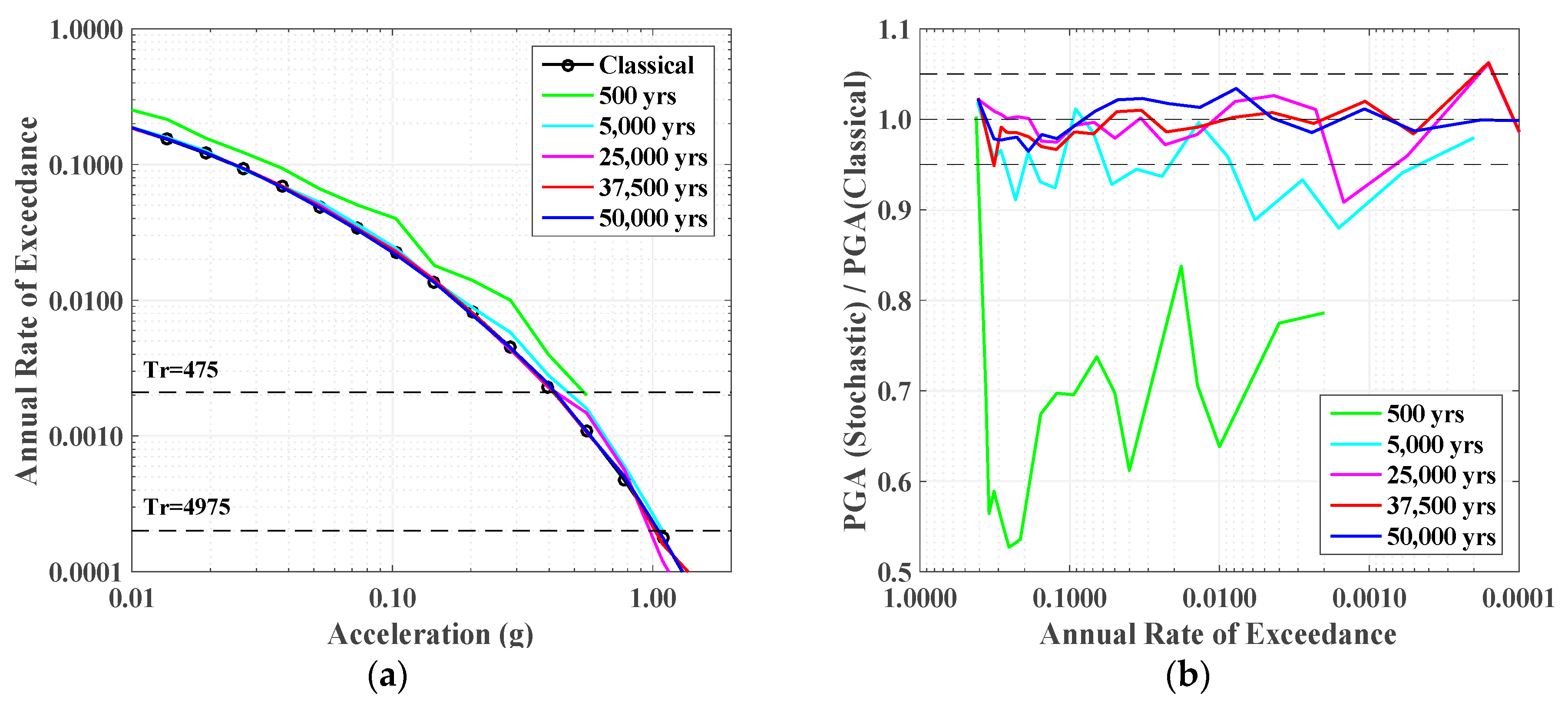
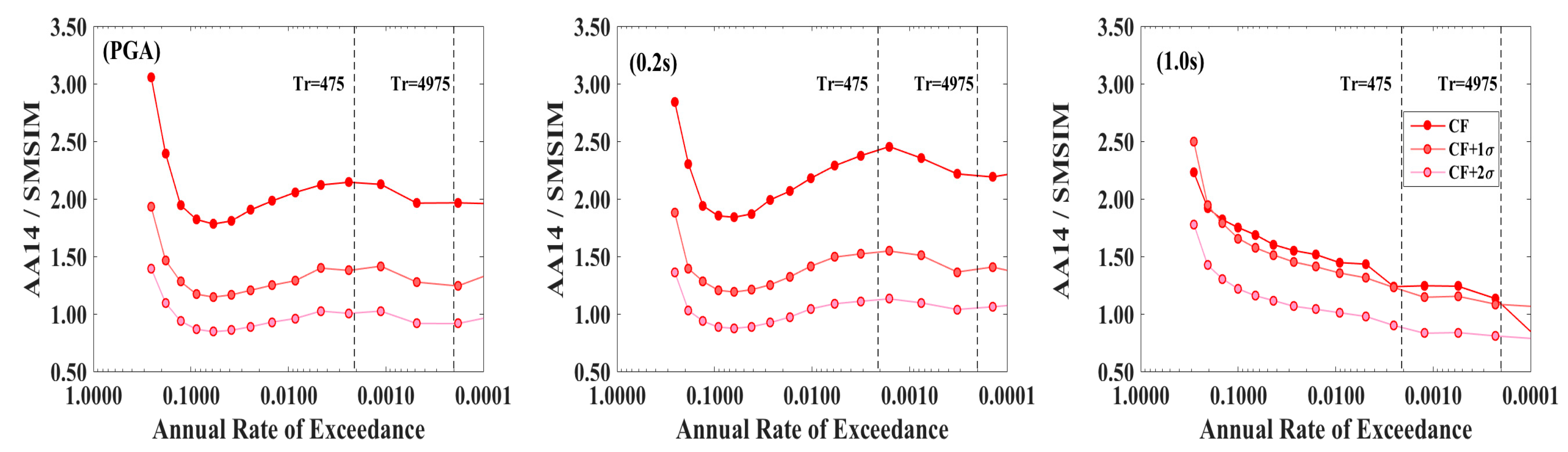
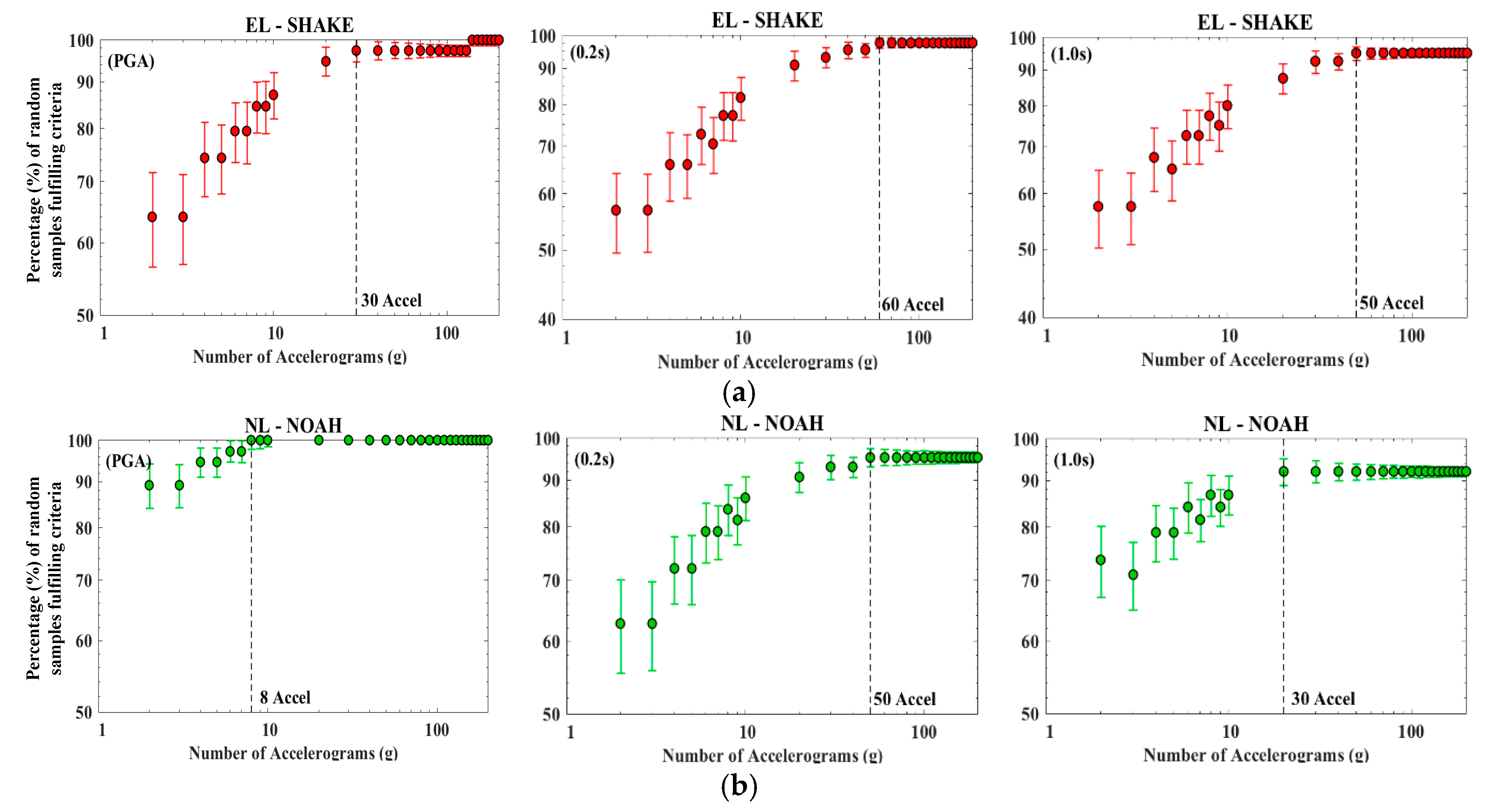
In order to calculate a fully probabilistic hazard curve on soil at the surface (or at any desired depth), [10,11] proposed three different approaches to calculate hazard on soil, consisting in the convolution of the site-specific hazard curve at the bedrock level with simple to more complex descriptions of the site amplification function. These approaches provide more precise surface ground-motion hazard estimates than those found by means of standard GMPEs for generic soil conditions. These three different methods are: (1) Full Convolution of the reference rock hazard curve with the NL amplification function, AF ( f , S a r ), and its variability. (2) PSHA with a Site-Specific GMPE (i.e., with the generic site term of the original GMPE being replaced by a site-specific term, S, derived from the site-specific amplification functions, A F ( f , S a r ), and the original aleatory variability being also modified to account for the actual variability in the site-specific amplification function). (3) Analytical estimate of the soil hazard convolving the probabilistic rock hazard curve with a statistical description of the non-linear site response and its variability.
In the present work, we decided to use the third approach, which is the simplest one to implement. The “Analytical Estimate of the Soil Hazard” method (AM) provides a simple, closed-form solution that appropriately modifies the hazard results at the rock level to obtain the hazard curve on soil. Under several assumptions, as discussed in their paper, [10,11] stated that the acceleration on soil, S a s ( f ) , can be predicted from the acceleration on rock, S a r ( f ) ,   as follows:
  l n ( S a s ( f ) ) = C 0 + ( C 1 + 1 )   l n ( S a r ( f ) )  
The amplification function is:
  A F ( f ) = S a s ( f ) S a r ( f )  
Equation 4 simply corresponds to a log-linear dependence of the amplification factor A F ( f ) in Equation (4) and the loading level S a r ( f ) in the form l n ( A F ( f ) )   =   C 0   +   C 1   l n ( S a r ( f ) ) , with a variability described by a standard deviation σ l n ( A F ( f )), as in Figure 15.
They also assumed that the rock hazard curve H C ( S a r ( f ) ) may be locally described with a power law dependence on the spectral acceleration, as follows:
  H C ( S a r ( f ) )   =   H 0 · S a r k 1  
By convolving the rock hazard curve with the lognormal distribution of the site amplification factor and its linear dependence on the loading level, they could then derive a closed-form expression for the hazard curve at soil site, as follows:
  H C ( S a s ( f ) ) = H C ( S a r ( f ) ) · e ( 1 2 k 1 2 σ 2 ( C 1 + 1 ) 2 )  
where σ corresponds to the standard deviation of the amplification function in log-normal scale, σ l n ( A F ( f ) ) , and the spectral acceleration on rock, S a r ( f ) , is related to the spectral acceleration on soil, S a s ( f ) , through the corresponding median amplification curve A F ( f , S a r ) . In the case where the uncertainty can be associated to the rock hazard curve (e.g., when a logic tree is used with different GMPEs), the resulting uncertainty in the soil site hazard curve may be written, as proposed by [11]:
  σ l n S a s ( f ) ( C 1 + 1 ) 2 σ l n S a r ( f ) 2 + σ l n A F ( f ) 2  
The first step in the proposed procedure consists in calculating the amplification functions, A F ( f ) , in the response spectra domain for all input ground motions and for each site response approach (SHAKE91 and NOAH), and then proceed to fit piecewise linear regressions to obtain the values of the coefficients C0 and C1, together with the associated variability, σ l n ( A F ( f ) ) . The results are illustrated in Figure 15 for the two site-response codes and for the three considered spectral periods. It is interesting to notice that non-linear behavior is observed even at relatively large spectral periods (~1.0 s)—for large loading levels—and also at short periods (PGA and 0.2 s) from rather low input acceleration levels (blue regression lines in Figure 15a,b).
The explanation for the former (long period non-linear behavior) can be related to the low fundamental frequency of the site (~[0.6–0.7] Hz): everything beyond that frequency is primarily controlled by the site response, and the large velocity contrast at ~200 m depth is likely to generate significant strains over the whole soil column. The latter observation, however, seems more likely to be related to the dependence of amplification factor on the response spectra on the actual frequency contents of the input waveform, leading to the magnitude dependence of the response spectral amplification, as reported in [58], than to a true NL behavior at very low strains, which cannot be identified in the corresponding Fourier domain amplifications [60].
The regression coefficients are listed in Table 3 together with their standard deviations. The hazard curves on soil can now be estimated according to Equation (6). It is worth discussing the limitations of this simplified analytical method (AM), as already acknowledged by [11]. The functional form provided in Equation (6) presents numerical limitations when the argument of the exponential is too large, i.e., when C1 is close to −1.0, and/or when the variability of the amplification factor (σ) is large. The former situation does occur at Euroseistest for high acceleration levels (green lines in Figure 15a,b), which corresponds to the saturation of surface ground motion displayed in Figure 12.
The hazard curves obtained are presented in Figure 16a (SHAKE91) Figure 16b (NOAH). In most cases of this particular example (all except in Figure 16b, i.e., for the NL code NOAH at PGA level), the nonlinearity is so important for both site response models, that the AM approach is not even capable to provide hazard curves results for the most common 475 years return period: C1 values are getting to close to −1.0, where Equation (6) diverges. This limitation is actually one of the main drawbacks of the AM approach, which cannot be used in the case of strong non-linearity. Also, as acknowledged by [11], the AM should be used with caution when the correction factor in Equation (6) takes on values that are greater than 10 (which may also result from a large variability on the amplification factor for different waveforms).

5.4. Robustness of the A F ( f ) Prediction

Another issue that may be discussed that is related to the accuracy and performance of the model, is the required amount of accelerograms to robustly predict the median of the amplification function l n ( A F ) . Bazzurro, P. [10] proposed that “the number of records, n, needed to keep the standard error of the median of l n ( A F ( f ) ) at any spectral acceleration level within a specified fractional accuracy, ζ, is approximately (Strictly, Equation (9) is valid for the median l n   A F ( f ) at a lognormal spectral-acceleration level corresponding to the sample median of the spectral-acceleration values used to produce the piece-wise regression. The standard error of the median of l n ( A F ) grows at values that are away from the average. So, to maximize accuracy, the record intensities should be chosen in the appropriate l n   S a r ( f ) neighborhood (see [10]).) given by” Equation (8):
  n = [ σ l n A F ( f ) ζ ] 2  
The standard deviation of the median of l n ( A F ) is in both cases (SHAKE91 and NOAH) and at all spectral periods significantly lower than 0.3 (Figure 15a,b and Table 3, most values between 0.01 and 0.2). The criterion defined by [10] in page 2099 is therefore fulfilled: “Given that the residual standard deviation of the quadratic model in l n   S a r ( f ) is 0.3 or less across the entire frequency range, the median value of A F ( f ) associated with a given S a r ( f ) on rock can be estimated within ±10% (i.e., ζ = 0.1) by using not more than 10 records”.
To test this assertion, we randomly selected from 2 to 200 accelerograms (1000 times each) in our set of stochastic time histories and for different S a r ( f ) bins, S a r ( f ) bins = [0.001:0.001:0.01; 0.01:0.01:0.1; 0.1:0.1:2]. Posteriorly, we calculated efficiency curves showing the percentage of random samples where the number of accelerograms, n , predicted a median l n   A F ( f ) within a 10% error margin (with respect to median l n   A F ( f ) , estimated from the full set of stochastic time series; Figure 17 and Table 4). One can observe that the number of accelerograms that is required is larger using SHAKE91 than using NOAH. This is due to the larger variability of SHAKE91 data with respect to NOAH data. Hence, more accelerograms are needed for a robust estimation. From this particular example, we determine that an amount of 60 accelerograms per acceleration bin S a r ( f ) are required to robustly predict the median of the amplification function l n ( A F ) . The different centers of the S a r ( f ) bins that were used are displayed in Figure 18 and Figure 19.
We consider that the differences between [10,11] work and this study, might be associated to the following reasons: (1) The authors in [10,11] calculated the “true” reference median l n ( A F ) based on only 78 ground motion records along all of the acceleration levels, S a r ( f ) , while in our case, we calculated the “true” reference median, l n ( A F ) , with more than ~21,800 ground motion time histories. Authors in [10,11] might have been calculating statistics on a sample too small. (2) Since both studies are site-specific studies, it is very likely that the minimum number of records to estimate the median l n ( A F ) with a given accuracy is expected to be different. However, we found that, in our case, the expression in Equation (8) is insufficient and under conservative, and such differences cannot be explained by the selected Mw and Dhyp range of the accelerograms, since in their study, the authors considered records with magnitudes and distances that were between Mw = [5.0–7.4] and Dhyp = [0.1–142] km, while we explore the magnitudes and distances between Mw = [4.7–7.9] and Dhyp = (1–150).
With respect to the robustness of the standard deviation of AF ( f , S a r ) , nothing was said by the authors. We decided to explore the behavior of the standard deviation while considering 30, 50, and then whole set of accelerograms. Figure 18 and Figure 19 display the amplification factor, AF ( f , S a r ) , (top) and its standard deviation (bottom), versus the input hazard on hard rock, S a r ( f ) , using SHAKE91 and NOAH results, respectively. The median standard deviation as a function of the input hazard on hard rock, S a r ( f ) , does not vary significantly when increasing the number of accelerograms, for both SHAKE91 and NOAH results. The apparent larger variation at high input acceleration levels is due to the lack of data on such acceleration levels.

6. Discussion

The direct comparison of both approaches in Figure 20 shows that the AM and SM hazard curves present a good fit at all available return periods for the three studied spectral periods. Nevertheless, despite this good fit, the above-mentioned numerical limitation of the AM method prevents this study from performing such comparison even at the most common 475 years return period, which raises questions about the effectiveness of the AM approach for the incorporation of site effects in site-specific PSHA. It is important to emphasize that this limitation will only affect sites with strong nonlinear and/or high seismic demands such as the Euroseistest site. The vertical asymptotes of the hazard curves on soil in Figure 20 correspond, for each spectral period, to the slope (green) in Figure 12, and it therefore corresponds to a non-linear saturation effect of the ground motion at the surface under strong shaking, as it can be better appreciated in Figure 21.
These results also show that the code-to-code variability introduces much more uncertainty on the hazard estimates than the method-to-method (AM, SM) variability. The use of SHAKE91 leads to larger PGA values for return periods that are larger than 100 years, while the use of NOAH leads to larger spectral accelerations for all of the return periods at intermediate and long spectral periods (0.2 s and 1.0 s). It is interesting to notice that nonlinear behavior is observed, even at relatively large spectral periods (1.0 s) and low return periods. However, the deamplification behavior with respect to rock occurs only at short periods (PGA, 0.2 s), while at longer period (1.0 s), amplification can be observed for all explored return periods. This is simply because the (1.0 s) period is close to the fundamental period of the site (~1.5 s), where linear amplification is strong (close to a factor of 10). Hence, the nonlinearity due to the soil shear modulus degradation and larger damping (induced under strong strain levels) is not strong enough to generate deamplification with respect to the ground motion on rock.
Concerning the ground motion variability analysis, the standard deviation of the ground motion on soil, σ S a s ( f ) , remains in both cases (SHAKE91 and NOAH) of the same order of magnitude at low ground motion levels (Figure 13a), and it is larger for SHAKE91 than for NOAH at strong ground motion levels (Figure 13c). This can be partially explained by the larger variability of amplification A F ( f ) using SHAKE than NOAH (Figure 15, Table 3, σ ( A F ) ). Additionally, our numerical results are in qualitative agreement with observations from real recordings on soil and rock [57,58], where the standard deviation on soil, σ S a s ( f ) , is smaller than the standard deviation on rock, σ S a r ( f ) , for all ground motion levels (see Figure 13). Currently, this phenomenon is presumed to be due to nonlinearity of the soil response during severe shaking [11], and also the effect of a lower damping at low strain levels on rock that makes the ground motion more sensitive to the input motion.
Furthermore, we compared the predictions with current available data at the site. Figure 21 plots the spectral acceleration on soil, as a function of the corresponding input spectral acceleration on rock, for both nonlinear codes tested, together with recordings from the Euroseistest database [17]. The same amount of observed earthquakes recordings (28 records) are used at the three different spectral periods, but accelerations on rock below 0.001g are not displayed.
From visual inspection, the few observations that are available at low/intermediate ground motion levels are roughly within the range predicted by the two models. We can thus expect the actual hazard curve of the site to be comprised between the two proposed hazard models. SHAKE91 might better predict site surface motion for low input ground motion levels [ S a r ( f )   < 0.01 g], while NOAH predictions might be better for intermediate input ground motion levels [0.01 g ≤ S a r ( f )   ≤ 0.1 g]. However, many more recordings would be necessary to derive sound conclusions. For higher input acceleration levels [ S a r ( f )   > 0.1 g], nothing can be said, as they are no recordings. As some of the accelerations recorded are located outside the scatter range, it seems that the simulations somewhat underestimate the actual variability.

7. Conclusions

A comparison between two fully probabilistic methods to integrate site effects into PSHA has been presented along this work. We found that the analytical approximation of the full convolution method, AM, is computationally less expensive, but it breaks down in the case of strong non-linearity due to a numerical limitation (as for the Euroseistest site). On the other hand, the full probabilistic stochastic method, SM, requires much heavier computations, but it provides results over the full acceleration range, even when strong non-linearity occurs. Both of the methods provide comparable annual exceedance rates over their common validity range.
To build the hazard curves on soil, two different propagation codes were used to calculate the time histories on soil at the surface, EL-SHAKE91 [42,43,44] and NL-NOAH [45]. In the Euroseistest case study, the code-to-code variability is found to control the uncertainty on the hazard estimates, rather than the method-to-method variability (AM or SM). We found that the soil variability that was obtained as a result after performing the propagation is smaller than the input rock variability. This result is in qualitative agreement with observations from real recordings on soil and rock [57,58]. Currently, this phenomenon is presumed to be due to nonlinearity of the soil response during severe shaking [11]. We also found that the expression describing the minimum required amount of records proposed by [11] falls rather short in our case, being insufficient and under conservative, especially for capturing the whole variability of the site response. For this particular example, 8 to 60 records per acceleration bin on rock were needed to predict the amplification within a 10% error margin (with respect to the true amplification based on the full stochastic sample), for both propagation codes and at the three studies spectral periods (PGA, 0.2 s and 1.0 s).
By comparing the two models with real in-situ data, we observed that the few available recordings at the Euroseistest are within the acceleration range that was predicted by both site response models (EL and NL). However, more data might be needed to validate this observation.
We are aware that the selection of the synthetic time histories and the scaling procedure that we followed here might raise several questions that are related to the ‘true ground motion’ at the Euroseistest. However, the selection of the input time histories on rock is simply an intermediate step that, in our opinion, should not impact significantly the conclusions reached here. The accelerogram selection and generation process would impact the site nonlinear response in case of a deterministic study with one or only a few times series. We believe that the large number of computations performed here allows for considering that the results are statistically significant and quite robust with respect to the actual phase contents of the input rock time series. It must nevertheless be emphasized that the selection of accelerograms compatible to a given GMPE is still an open issue, which needs to be better addressed in the future. Recent works, such as those proposed by [55,60], allow for a more physical tuning of the source and crustal propagation parameters, while not warranting however to get the actual regional site and source parameters, neither avoiding the potential trade-off between some of them [38].
We are also aware that the nonlinear parameters that are assumed for the soil column (in particular the zero-cohesion) results in over-emphasizing the impact of the non-linearity of site response on the hazard curve, and thus limiting the validity domain of the AM approach. The present results, especially in terms of AM/SM comparison, are thus to be considered as an ‘extreme’ example for highly non-linear, thick soft site. It is likely that the validity domain of the AM approach would be much larger for shallow, high-plasticity clayey deposits.
Finally, we encourage the use of ground-motion simulations calibrated with real data to integrate site effects into PSHA, since models with different levels of complexity can be included (e.g., point source, extended source, 1D, 2D, and 3D site response analysis, kappa, hard rock …), and the corresponding variability of the site response can be quantified. In most practical cases, this is presently not possible with real data because of their scarcity at high acceleration levels.

Author Contributions

C.A., P.-Y.B. and C.B. conceived and designed the experiments; C.A. and J.-C.G. performed the experiments; C.A. and P.-Y.B. analyzed the data; C.A., J.-C.G., contributed/materials/analysis tools; C.A., P.-Y.B. and C.B. wrote the paper.

Funding

This work has been supported by a grant from Labex OSUG@2020 (Investissements d’avenir—ANR10 LABX56—http://www.osug.fr/labex-osug-2020/) and by the European STREST project (Harmonized approach to stress tests for critical infrastructures against natural hazards—http://www.strest-eu.org).

Acknowledgments

Special thanks are due to Benjamin Edwards, Adrián Rodriguez-Marek, Valerio Poggi and an anonymous reviewer for fruitful discussions. Also, special thanks to Fabian Bonilla for facilitating the nonlinear code NOAH and additional technical assistance on its usage, and to Fabrice Hollender for providing valuable geotechnical and site-specific data to build the nonlinear models. All ground-motion records used in this study were generated using Boore 2003 Stochastic Method and his open source code SMSIM (http://www.daveboore.com/). Hazard calculations on rock have been performed using the Openquake engine (http://www.globalquakemodel.org/), as well as the SHARE area source model (http://www.share-eu.org/). The post-processing toolkits developed by the GEM Foundation have been used. Special thanks to Geosciences (Switzerland) for the invitation to participate to this special issue.

Conflicts of Interest

The authors declare no conflict of interest.

References

  1. Kramer, S.L. Geotechnical Earthquake Engineering; Prentice Hall: New York, NY, USA, 1996. [Google Scholar]
  2. Bazzurro, P. Probabilistic Seismic Damage Analysis. Ph.D. Thesis, Stanford University, Stanford, CA, USA, August 1998. [Google Scholar]
  3. Bazzurro, P.; Cornell, C.A.; Shome, N.; Carballo, J.E. Three proposals for characterizing MDOF nonlinear seismic response. J. Struct. Eng. 1998, 124, 1281–1289. [Google Scholar] [CrossRef]
  4. Bazzurro, P.; Cornell, C.A. Vector-valued probabilistic seismic hazard analysis (VPSHA). In Proceedings of the 7th US National Conference on Earthquake Engineering, Boston, MA, USA, 21–25 July 2002; pp. 21–25. [Google Scholar]
  5. Lee, R.; Silva, W.J.; Cornell, C.A. Alternatives in evaluating soil-and rock-site seismic hazard. Seismol. Res. Lett. 1998, 69, 81. [Google Scholar]
  6. Lee, R.C. A Methodology to Integrate Site Response into Probabilistic Seismic Hazard Analysis; Site Geotechnical Services: Savannah, GA, USA, 2000. [Google Scholar]
  7. Tsai, C.C.P. Probabilistic seismic hazard analysis considering nonlinear site effect. Bull. Seismol. Soc. Am. 2000, 90, 66–72. [Google Scholar] [CrossRef]
  8. Cramer, C.H. Site-specific seismic-hazard analysis that is completely probabilistic. Bull. Seismol. Soc. Am. 2003, 93, 1841–1846. [Google Scholar] [CrossRef]
  9. Cramer, C.H. Erratum: Site-Specific Seismic-Hazard Analysis that is Completely Probabilistic. Bull. Seismol. Soc. Am. 2005, 95, 2026. [Google Scholar] [CrossRef]
  10. Bazzurro, P.; Cornell, C.A. Ground-motion amplification in nonlinear soil sites with uncertain properties. Bull. Seismol. Soc. Am. 2004, 94, 2090–2109. [Google Scholar] [CrossRef]
  11. Bazzurro, P.; Cornell, C.A. Nonlinear soil-site effects in probabilistic seismic-hazard analysis. Bull. Seismol. Soc. Am. 2004, 94, 2110–2123. [Google Scholar] [CrossRef]
  12. Papaspiliou, M.; Kontoe, S.; Bommer, J.J. An exploration of incorporating site response into PSHA—Part I: Issues related to site response analysis methods. Soil Dyn. Earthq. Eng. 2012, 42, 302–315. [Google Scholar] [CrossRef]
  13. Papaspiliou, M.; Kontoe, S.; Bommer, J.J. An exploration of incorporating site response into PSHA—Part II: Sensitivity of hazard estimates to site response approaches. Soil Dyn. Earthq. Eng. 2012, 42, 316–330. [Google Scholar] [CrossRef]
  14. Aristizábal, C.; Bard, P.Y.; Beauval, C. Site-specific PSHA: Combined effects of single station sigma, host-o-target adjustments and non-linear behavior. In Proceedings of the World Conference on Earthquake Engineering, Santiago, Chile, 9–13 January 2017. [Google Scholar]
  15. Aristizábal, C. Integration of Site Effects into Probabilistic Seismic Hazard Methods. Ph.D. Thesis, Université Grenoble Alpes, Grenoble, France, 2018. [Google Scholar]
  16. Campbell, K.W. Prediction of strong ground motion using the hybrid empirical method and its use in the development of ground-motion (attenuation) relations in eastern North America. Bull. Seismol. Soc. Am. 2003, 93, 1012–1033. [Google Scholar] [CrossRef]
  17. Pitilakis, K.; Roumelioti, Z.; Raptakis, D.; Manakou, M.; Liakakis, K.; Anastasiadis, A.; Pitilakis, D. The EUROSEISTEST Strong-Motion Database and Web Portal. Seismol. Res. Lett. 2013, 84, 796–804. [Google Scholar] [CrossRef]
  18. Woessner, J.; Laurentiu, D.; Giardini, D.; Crowley, H.; Cotton, F.; Grünthal, G.; Valensise, G.; Arvidsson, R.; Basili, R.; Demircioglu, M.B.; et al. The 2013 European seismic hazard model: Key components and results. Bull. Earthq. Eng. 2015, 13, 3553–3596. [Google Scholar]
  19. Liotier, Y. Modelisation des Ondes de Volume des Seismes de L’arc Ageen; DEA de l’Universite Joseph Fourier: Grenoble, France, 1989. [Google Scholar]
  20. Carver, D.; Bollinger, G.A. Aftershocks of the June 20, 1978, Greece earthquake: A multimode faulting sequence. Tectonophysics 1981, 73, 343–363. [Google Scholar] [CrossRef]
  21. Mountrakis, D.; Psilovikos, A.; Papazachos, B. The geotectonic regime of the 1978 Thessaloniki earthquakes. In The Thessaloniki, Northern Greece, Earthquake of June 20, 1978 and Its Seismic Sequence; Papazachos, B.C., Carydis, P.G., Eds.; Technical Chamber of Greece: Thessaloniki, Greece, 1983; pp. 11–27. [Google Scholar]
  22. Jongmans, D.; Pitilakis, K.; Demanet, D.; Raptakis, D.; Riepl, J.; Horrent, C.; Tsokas, G.; Lontzetidis, K.; Bard, P.Y. EURO-SEISTEST: Determination of the geological structure of the Volvi basin and validation of the basin response. Bull. Seismol. Soc. Am. 1998, 88, 473–487. [Google Scholar]
  23. Raptakis, D.; Chávez-Garcıa, F.J.; Makra, K.; Pitilakis, K. Site effects at Euroseistest—I. Determination of the valley structure and confrontation of observations with 1D analysis. Soil Dyn. Earthq. Eng. 2000, 19, 1–22. [Google Scholar] [CrossRef]
  24. Chávez-Garcıa, F.J.; Raptakis, D.; Makra, K.; Pitilakis, K. Site effects at Euroseistest—II. Results from 2D numerical modeling and comparison with observations. Soil Dyn. Earthq. Eng. 2000, 19, 23–39. [Google Scholar] [CrossRef]
  25. Manakou, M.V.; Raptakis, D.G.; Chávez-García, F.J.; Apostolidis, P.I.; Pitilakis, K.D. 3D soil structure of the Mygdonian basin for site response analysis. Soil Dyn. Earthq. Eng. 2010, 30, 1198–1211. [Google Scholar] [CrossRef]
  26. Pitilakis, K.; Raptakis, D.; Lontzetidis, K.; Tika-Vassilikou, T.; Jongmans, D. Geotechnical and Geophysical Description of Euro-Seistest, Using Field, Laboratory Tests and Moderate Strong Motion Recordings. J. Earthq. Eng. 1999, 3, 381–409. [Google Scholar] [CrossRef]
  27. Riepl, J.; Bard, P.Y.; Hatzfeld, D.; Papaioannou, C.; Nechtschein, S. Detailed evaluation of site-response estimation methods across and along the sedimentary valley of Volvi (EURO-SEISTEST). Bull. Seismol. Soc. Am. 1998, 88, 488–502. [Google Scholar]
  28. Maufroy, E.; Chaljub, E.; Hollender, F.; Kristek, J.; Moczo, P.; Klin, P.; Priolo, E.; Iwaki, A.; Iwata, T.; Etienne, V.; et al. Earthquake ground motion in the Mygdonian basin, Greece: The E2VP verification and validation of 3D numerical simulation up to 4 Hz. Bull. Seismol. Soc. Am. 2015, 105, 1398–1418. [Google Scholar] [CrossRef]
  29. Maufroy, E.; Chaljub, E.; Hollender, F.; Bard, P.Y.; Kristek, J.; Moczo, P.; De Martin, F.; Theodoulidis, N.; Manakou, M.; Guyonnet-Benaize, C.; et al. 3D numerical simulation and ground motion prediction: Verification, validation and beyond—Lessons from the E2VP project. Soil Dyn. Earthq. Eng. 2016, 91, 53–71. [Google Scholar]
  30. Maufroy, E.; Chaljub, E.; Theodoulidis, N.P.; Roumelioti, Z.; Hollender, F.; Bard, P.Y.; De Martin, F.; Guyonnet-Benaize, C.; Margerin, L. Source-Related Variability of Site Response in the Mygdonian Basin (Greece) from Accelerometric Recordings and 3D Numerical Simulations. Bull. Seismol. Soc. Am. 2017, 107, 787–808. [Google Scholar] [CrossRef]
  31. Cotton, F.; Scherbaum, F.; Bommer, J.J.; Bungum, H. Criteria for selecting and adjusting ground-motion models for specific target regions: Application to central Europe and rock sites. J. Seismol. 2006, 10, 137–156. [Google Scholar]
  32. Van Houtte, C.; Drouet, S.; Cotton, F. Analysis of the origins of κ (kappa) to compute hard rock to rock adjustment factors for GMPEs. Bull. Seismol. Soc. Am. 2011, 101, 2926–2941. [Google Scholar] [CrossRef]
  33. Delavaud, E.; Scherbaum, F.; Kuehn, N.; Allen, T. Testing the global applicability of ground-motion prediction equations for active shallow crustal regions. Bull. Seismol. Soc. Am. 2012, 102, 707–721. [Google Scholar] [CrossRef]
  34. Biro, Y.; Renault, P. Importance and impact of host-to-target conversions for ground motion prediction equations in PSHA. In Proceedings of the 15th World Conference on Earthquake Engineering, Lisbon, Portugal, 24–28 September 2012; pp. 24–28. [Google Scholar]
  35. Anderson, J.G.; Hough, S.E. A model for the shape of the Fourier amplitude spectrum of acceleration at high frequencies. Bull. Seismol. Soc. Am. 1984, 74, 1969–1993. [Google Scholar]
  36. Akkar, S.; Sandıkkaya, M.A.; Bommer, J.J. Empirical ground-motion models for point-and extended-source crustal earthquake scenarios in Europe and the Middle East. Bull. Earthq. Eng. 2014, 12, 359–387. [Google Scholar]
  37. Laurendeau, A.; Bard, P.-Y.; Hollender, F.; Perron, V.; Foundotos, L.; Ktenidou, O.J.; Hernandez, B. Derivation of consistent hard rock (1000 <VS <3000 m/s) GMPEs from surface and down-hole recordings: Analysis of KiK-net data. Bull. Earthq. Eng. 2018, 16, 2253–2284. [Google Scholar]
  38. Bard, P.-Y.; Bora, S.S.; Hollender, F.; Laurendeau, A.; Traversa, P. Are the standard Vs30-kappa host-to-target adjustments the best way to get consistent hard-rock ground motion prediction? In Proceedings of the 2nd International Workshop on “Best Practices in Physics-Based Fault Rupture Models for Seismic Hazard Assessment of Nuclear Installations: Issues and challenges towards Full Seismic Risk Analysis”, Cadarache-Château, France, 14–16 May 2018.
  39. Pagani, M.; Monelli, D.; Weatherill, G.; Danciu, L.; Crowley, H.; Silva, V.; Henshaw, P.; Butler, L.; Nastasi, M.; Panzeri, L.; et al. OpenQuake engine: An open hazard (and risk) software for the global earthquake model. Seismol. Res. Lett. 2014, 85, 692–702. [Google Scholar] [CrossRef]
  40. Boore, D.M. Simulation of ground motion using the stochastic method. In Seismic Motion, Lithospheric Structures, Earthquake and Volcanic Sources; Birkhäuser: Basel, Switzerland, 2006; pp. 635–676. [Google Scholar]
  41. Boore, D.M. SMSIM: Fortran Programs for Simulating Ground Motions from Earthquakes; version 2.3; US Department of the Interior: Washington, DC, USA; US Geological Survey: Reston, VA, USA, 2005.
  42. Schnabel, P.B. SHAKE a Computer Program for Earthquake Response Analysis of Horizontally Layered Sites; EERC Report; University of California: Berkeley, CA, USA, 1972. [Google Scholar]
  43. Idriss, I.M.; Sun, J.I. User’s Manual for SHAKE91: A Computer Program for conducting Equivalent Linear Seismic Response Analyses of Horizontally Layered Soil Deposits; Center for Geotechnical Modeling, Department of Civil and Environmental Engineering, University of California: Davis, CA, USA, 1993. [Google Scholar]
  44. Schnabel, P.B.; Lysmer, J.; Seed, H.B. SHAKE-91: Equivalent Linear Seismic Response Analysis of Horizontally Layered Soil Deposits; The Earthquake Engineering Online Archive NISEE E-Library: Berkeley, CA, USA, 1993. [Google Scholar]
  45. Bonilla, L.F. NOAH: Users Manual; Institute for Crustal Studies, University of California: Santa Barbara, CA, USA, 2001. [Google Scholar]
  46. Régnier, J.; Bonilla, L.F.; Bard, P.Y.; Bertrand, E.; Hollender, F.; Kawase, H.; Sicilia, D.; Arduino, P.; Amorosi, A.; Asimaki, D.; et al. International benchmark on numerical simulations for 1D, non-linear site response (PRENOLIN): Verification phase based on canonical cases. Bull. Seismol. Soc. Am. 2016, 106, 2112–2135. [Google Scholar] [CrossRef]
  47. Régnier, J.; Bonilla, L.F.; Bard, P.Y.; Bertrand, E.; Hollender, F.; Kawase, H.; Sicilia, D.; Arduino, P.; Amorosi, A.; Asimaki, D.; et al. PRENOLIN: International Benchmark on 1D Nonlinear Site-Response Analysis—Validation Phase Exercise. Bull. Seismol. Soc. Am. 2018, 108, 876–900. [Google Scholar] [CrossRef]
  48. Global Earthquake Model. The OpenQuake-Engine User Manual; Technical Report; GEM: Pavia, Italy, 2017. [Google Scholar]
  49. Ktenidou, O.J.; Abrahamson, N.A. Empirical estimation of high-frequency ground motion on hard rock. Seismol. Res. Lett. 2016, 87, 1465–1478. [Google Scholar] [CrossRef]
  50. Kottke, A.R. VS30-k0 relationship implied by ground motion models? In Proceedings of the 16th World Conference on Earthquake Engineering, Santiago, Chile, 9–13 January 2017.
  51. Al Atik, L.; Kottke, A.; Abrahamson, N.; Hollenback, J. Kappa (κ) scaling of ground-motion prediction equations using an inverse random vibration theory approach. Bull. Seismol. Soc. Am. 2014, 104, 336–346. [Google Scholar] [CrossRef]
  52. Okada, Y.; Kasahara, K.; Hori, S.; Obara, K.; Sekiguchi, S.; Fujiwara, H.; Yamamoto, A. Recent progress of seismic observation networks in Japan—Hi-net, F-net, K-NET and KiK-net—. Earth Planets Space 2004, 56, 15–28. [Google Scholar] [CrossRef]
  53. Ktenidou, O.J.; Abrahamson, N.A.; Drouet, S.; Cotton, F. Understanding the physics of kappa (κ): Insights from a downhole array. Geophys. J. Int. 2015, 203, 678–691. [Google Scholar]
  54. Atkinson, G.M.; Boore, D.M. Ground-motion relations for eastern North America. Bull. Seismol. Soc. Am. 1995, 85, 17–30. [Google Scholar]
  55. Zandieh, A.; Pezeshk, S.; Campbell, K.W. An Equivalent Point-Source Stochastic Simulation of the NGA-West2 Ground-Motion Prediction Equations. Bull. Seismol. Soc. Am. 2018, 108, 815–835. [Google Scholar] [CrossRef]
  56. Silva, W.J.; Lee, R.; McGuire, R.K.; Cornell, C.A. A comparison of methodologies to achieve a site-specific PSHA. Seismol. Res. Lett. 2000, 71, 247. [Google Scholar]
  57. Abrahamson, N.A.; Sykora, D. Variations of ground motions across individual sites. In Proceedings of the DOE Natural Phenomena Hazards Mitigation Conference, Atlanta, GA, USA, 19–22 October 1993; pp. 192–198. [Google Scholar]
  58. Toro, G.R.; Abrahamson, N.A.; Schneider, J.F. Model of strong ground motions from earthquakes in central and eastern North America: Best estimates and uncertainties. Seismol. Res. Lett. 1997, 68, 41–57. [Google Scholar] [CrossRef]
  59. Al Atik, L.; Abrahamson, N. Nonlinear site response effects on the standard deviations of predicted ground motions. Bull. Seismol. Soc. Am. 2010, 100, 1288–1292. [Google Scholar] [CrossRef]
  60. Stafford, P.J.; Rodriguez-Marek, A.; Edwards, B.; Kruiver, P.P.; Bommer, J.J. Scenario Dependence of Linear Site-Effect Factors for Short-Period Response Spectral Ordinates. Bull. Seismol. Soc. Am. 2017, 107, 2859–2872. [Google Scholar]
Figure 1. (a) Map showing the broader region of occurrence of the 20 June 1978 (M6.5) earthquake sequence. Epicenter and focal mechanism [19] of the mainshock (red) and epicenters of the largest events of the sequence (green, yellow) [20] are also depicted. Dotted lines mark the Mygdonian graben and surface ruptures after the 1978 earthquake [21] are shown as red lines. (b) Three-dimensional (3D) model of the Mygdonian basin geological structure [25]. (Figures from http://euroseisdb.civil.auth.gr/geotec).
Geosciences 08 00285 g001
Figure 2. (a) One-dimensional (1D) shear wave, Vs, and compressive wave, Vp, velocity profiles between TST0 and TST196 stations, located at the middle of the Euroseistest basin, at surface and 196 m depth, respectively. (b) Euroseistest shear modulus and (c) damping ratio degradation curves [27].
Geosciences 08 00285 g002
Figure 3. Target hazard curve on standard rock (VS30 = 800 m/s) at the Euroseistest calculated using Akkar et al., 2014 Ground Motion Prediction Equations (GMPE) (AA14) for three different spectral periods (PGA, 0.2 s, 1.0 s).
Geosciences 08 00285 g003
Figure 4. Hazard curves at Euroseistest, for three different spectral periods (PGA, 0.2 s, 1.0 s); blue: standard rock (VS30 = 800 m/s); green: hard rock (2600 m/s), calculated from the hazard curves on standard rock scaled with LA17 host-to-target (HTT) adjustment factors.
Geosciences 08 00285 g004
Figure 5. (ae) Truncated Gutenberg-Richter recurrence models derived from five different stochastic catalog lengths (500, 5000, 25,000, 35,500, and 50,000 years), compared with the original recurrence model of the source zone GRAS390 in the SHARE model. (f) The 5 recurrence curves obtained are superimposed to the original recurrence model.
Geosciences 08 00285 g005
Figure 6. (a) Hazard curves built from five earthquake catalogs with increasing lengths (from 500 to 50,000 years). (b) Ratio between the acceleration obtained from the Monte Carlo method and the expected acceleration, interpolated for given annual rates.
Geosciences 08 00285 g006
Figure 7. Hazard curves at the Euroseistest site for three different spectral periods (PGA, 0.2 s, 1.0 s), applying AA14 GMPE (blue for standard rock, green for hard rock—with HTT adjustments) or built from stochastic time histories on hard rock generated using SMSIM code (Vs = 2600 m/s, κ0 = 0.024 s, Δσ = 30 ± 0.68 bars, CAF(f) from [26]).
Geosciences 08 00285 g007
Figure 8. (a) Correction factors or ratios between synthetic accelerations and accelerations predicted by AA14 (adjusted at VS30 = 2600 m/s), for a series of magnitudes at different spectral periods: median ± one standard deviation of all available ratios for a given magnitude (Mw), μ is the median of all median correction factors when considering all magnitudes, and σ the corresponding standard deviation. (b) Variation of the correction factor with spectral period estimated over all magnitudes and distances: black solid line: interpolated frequency-dependent median correction factor; dashed line: median + one standard deviation; dot-dashed: median + two standard deviations. (c) Example of an Mw = 7.9 accelerogram generated using SMSIM (red) and then scaled by the interpolated median + two standard deviations correction factor (black).
Geosciences 08 00285 g008
Figure 9. In black, hazard curves for three spectral periods (PGA, 0.2 s, 1.0 s) built from SMSIM stochastic time histories scaled by the: (a) Median correction factor (CF), (b) Median + one standard deviation correction factor (CF+1σ), (c) Median + two standard deviation correction factor (CF+2σ). Also superimposed the hazard curves obtained with AA14 at VS30 = 800 m/s (blue), hazard curves obtained with AA14 corrected at VS30 = 2600 m/s (green), and hazard curves derived from SMSIM original time histories (red).
Geosciences 08 00285 g009
Figure 10. AA14 (2600 m/s)/SMSIM hazard curve ratios for three different spectral periods (PGA, left; 0.2 s, middle; 1.0 s, right), showing the fit of the hazard curve built from scaled stochastic time histories to the target hazard curve, using three different correction factors CF, CF+1σ, and CF+2σ. The best fit is obtained using the scaling factor CF+2σ at all spectral periods.
Geosciences 08 00285 g010
Figure 11. Mean spectral acceleration decay with respect to distance (km) predicted by AA14 · HTT ± 2σ (corrected for hard rock using HTT factors) for three different spectral periods (PGA, 0.2 s, 1.0 s), superimposed to the original SMSIM accelerations for hard rock (blue dots) and the scaled accelerations after applying a correction factor of CF+2σ (red dots) for events of Mw = [4.7, 6.5, 7.5].
Geosciences 08 00285 g011aGeosciences 08 00285 g011b
Figure 12. Spectral acceleration on soil Vs. Spectral acceleration on rock, for three different spectral periods (PGA, 0.2 s and 1.0 s); (a) Equivalent-linear (EL) results (SHAKE91); (b) Non-linear (NL) results (NOAH).
Geosciences 08 00285 g012
Figure 13. Probability density function (PDF) of the ground motion acceleration (PGA) on hard rock (blue) and on soil after performing 1D site response analysis using SHAKE91 (red) and NOAH (green) for different ranges of magnitudes (columns) and distances (rows).
Geosciences 08 00285 g013
Figure 14. Hazard curves calculated using the Full Probabilistic Stochastic Method (SM), for three different spectral periods (PGA, 0.2 s, 1.0 s). Time histories on: hard rock (VS30 = 2600 m/s, black), soft soil obtained with SHAKE91 site response code (red), soft soil obtained with NOAH site response code (green).
Geosciences 08 00285 g014
Figure 15. Trilinear piecewise regression models of A F ( f ) on S a r ( f ) for three different spectral periods (PGA, 0.2 s, 1.0 s): (a) Figures built using the accelerograms propagated with EL-SHAKE91. (b) Regression on the accelerograms propagated with NL-NOAH. The regression coefficients are indicated inside each plot (for each linear segment), see Table 3.
Geosciences 08 00285 g015aGeosciences 08 00285 g015b
Figure 16. Hazard curves on soil estimated with the analytical approximation method (AM), for three different spectral periods (PGA, 0.2 s and 1.0 s). (a) Hazard curve on rock and soil derived from SHAKE91 accelerograms. (b) hazard curve on soil derived from NOAH accelerograms. The blue, red and green points correspond to the different regression sections used to modify the original hazard curve (see Figure 15a). Hazard curves on hard rock (black).
Geosciences 08 00285 g016
Figure 17. (a) Efficiency curves: the median of A F ( f ) is estimated from n accelerograms randomly selected in our set of stochastic time histories, this is repeated 1000 times, and the percentage of samples where median A F ( f ) is within a 10% error with respect to the true median value (estimated over the full set of time histories) is determined. n varies between 2 and 200. (a) SHAKE case; (b) NOAH case.
Geosciences 08 00285 g017
Figure 18. Amplification factor, A F ( f ) , (top) and standard deviation (bottom), versus input hazard on hard rock, S a r ( f ) , derived using n accelerograms from the 1D SHAKE91 propagation (randomly sampled): (a) n = 30 accelerograms; (b) n = 60 accelerograms, (c) n = a l l accelerograms. The different colors correspond to the S a r ( f ) bins used to calculate the standard deviation.
Geosciences 08 00285 g018
Figure 19. Amplification factor, A F ( f ) , (top) and standard deviation (bottom), versus input hazard on hard rock, S a r ( f ) , derived using n accelerograms from the 1D NOAH propagation (randomly sampled): (a) n   =   30 accelerograms; (b)   n   =   60 accelerograms, (c) n = All accelerograms. The different colors correspond to the S a r ( f ) bins used to calculate the standard deviation.
Geosciences 08 00285 g019
Figure 20. Hazard curves on hard rock (blue) and soil using the equivalent-linear SHAKE91 simulations (red) and nonlinear NOAH simulations (green) for both AM (points) and SM (solid line) methods, at three different spectral periods (PGA, 0.2 s and 1.0 s).
Geosciences 08 00285 g020
Figure 21. Equivalent-linear (SHAKE91, red) and nonlinear (NOAH, green) predicted accelerations compared with data recorded at Euroseistest (yellow), for three different spectral periods (PGA, 0.2 s and 1.0 s).
Geosciences 08 00285 g021
Table 1. Material properties of the Euroseistest soil profile used on this study to perform the different site response calculations.
LayerSoil TypeDepth (m)Vs (m/s)Vp (m/s)ρ (kg/m3)Qϕ (°)Ko (adm)
1Silty Clay Sand0.01441524207714.4470.26
2Silty Sand*5.51771583208317.7190.67
3Lean Clay17.62641741209726.4190.68
4Fat Clay54.23881952211738.8270.54
5Silty Clay81.25262200215152.6420.33
6Weathered Rock131.17012520221570.1690.07
7Hard Rock183.0260045002446---
* Water table at 1 m depth. Vs: shear wave velocity. Vp: Compressive wave velocity. ρ: soil density. Q: Anelastic attenuation factor. ϕ: Friction angle. Ko: Coefficient of earth at rest.
Table 2. Host-to-target adjustments factors derived using LA17 hazard curves from a standard rock (VS30 = 800 m/s) to the Euroseistest hard rock (VS30 = 2600 m/s).
Spectral Period (s)PGA0.050.10.20.51.02.0
HTT Adjustment Factors0.470.450.380.510.700.780.86
Table 3. Intercept (C0), slope (C1), and standard deviation (σ) of the piecewise-linear regression models (PLM) for A F ( f ) vs. S a r ( f ) .
Spectral Period (s)Piecewise-Linear ModelsSHAKE91NOAH
C0C1 σ C0C1 σ  
PGAPLM 1 (Blue)0.7487−0.10890.150.5585−0.18330.11
PLM 2 (Red)−0.1202−0.29060.19−0.2539−0.36490.08
PLM 3 (Green)−1.3990−1.21400.19−1.6390−0.85940.08
(0.2)PLM 1 (Blue)0.2855−0.14750.191.0730−0.10200.12
PLM 2 (Red)−0.5356−0.40430.18−0.0906−0.47890.13
PLM 3 (Green)−1.1360−1.19700.27−0.9453−1.11720.35
(1.0)PLM 1 (Blue)0.8846−0.05610.271.7030−0.01700.11
PLM 2 (Red)0.4191−0.14380.140.7180−0.32980.22
PLM 3 (Green)0.9606−1.29000.082.2100−1.49300.26
Table 4. Minimum number of records, n, required to predict a median value of A F ( f ) within ±10% of the true value for three different spectral periods (PGA, 0.2 s and 1.0 s).
Coden, (PGA)n, (0.2 s)n, (1.0 s)
SHAKE91306050
NOAH85030

