A More Comprehensive Habitable Zone for Finding Life on Other Planets

Earth-Life Science Institute (ELSI), Tokyo Institute of Technology, Tokyo 152-8550, Japan
Geosciences 2018, 8(8), 280; https://doi.org/10.3390/geosciences8080280
Submission received: 13 June 2018
/
Revised: 25 July 2018
/
Accepted: 26 July 2018
/
Published: 28 July 2018
(This article belongs to the Special Issue Planetary Evolution and Search for Life on Habitable Planets)
Abstract
:The habitable zone (HZ) is the circular region around a star(s) where standing bodies of water could exist on the surface of a rocky planet. Space missions employ the HZ to select promising targets for follow-up habitability assessment. The classical HZ definition assumes that the most important greenhouse gases for habitable planets orbiting main-sequence stars are CO2 and H2O. Although the classical HZ is an effective navigational tool, recent HZ formulations demonstrate that it cannot thoroughly capture the diversity of habitable exoplanets. Here, I review the planetary and stellar processes considered in both classical and newer HZ formulations. Supplementing the classical HZ with additional considerations from these newer formulations improves our capability to filter out worlds that are unlikely to host life. Such improved HZ tools will be necessary for current and upcoming missions aiming to detect and characterize potentially habitable exoplanets.
1. Introduction
The habitable zone (HZ) is the circular region around a star (or multiple stars) where standing bodies of liquid water could exist on the surface of a rocky planet (e.g., [1,2]). Principally, the HZ is a navigational tool used by space missions to select promising planetary targets for follow-up observations. Although a planet located within the HZ is not necessarily inhabited, and additional information would be required to make such a determination, it remains the most useful roadmap for targeting potentially habitable worlds.
It is possible to invent alternate HZ definitions for solvents other than water [3]. Perhaps life thrives within the methane seas of Titan [4,5,6] and indeed this author hopes that a mission equipped to answer this question will visit the Saturnian moon someday. In contrast to the planets in our solar system, exoplanets cannot be visited so readily. Titan exo-analogues would be too far away from their stars and too faint for signs of life to be inferred with present day technology. The spectral signatures that can be expected from such worlds are also unknown. Therefore, the search for extraterrestrial life on exoplanets must presently be limited to a search for liquid water until future technological and biochemical breakthroughs can allow for a detailed exploration of planetary surfaces capable of hosting other solvents.
As suggested recently [2], the addition of the phrase “standing bodies of water” to the HZ definition emphasizes that habitable zone planets incapable of supporting more than seasonal trickles of surface water, like Mars, should not be considered for follow-up astrobiological observations. This is because any life residing within such small amounts of water would be unlikely to modify the atmosphere in a detectable manner. To be clear, such a search does not exclude potential ‘dune planets’, or desert worlds that exhibit water inventories smaller than the Earth [7,8], so long as sufficiently large bodies of water near the surface capable of modifying atmospheric spectra in a detectable way are present. Likewise, although moons like Europa and Enceladus contain large seas, these water bodies are capped by global ice layers that preclude any significant interactions between potential subsurface biota and the atmosphere. Thus, the HZ must also be defined for planets in which the atmosphere and surface water bodies are in direct contact.
It is also assumed that life requires a stable liquid or solid surface over which it can evolve. For this reason, it is not presently thought that gas giant atmospheres [9,10] present likely abodes for life. Chaotic atmospheric motions and complex chemical reactions may thwart life’s emergence. Until convincing evidence to the contrary arises, all discussion here assumes that rocky planets are the likely locales for alien life.
Even with such restrictions, the HZ can target a wide variety of worlds potentially consisting of life both like and unlike that on this planet. For example, in regions of higher pressure, the highest temperature sustainable by Earth life is ~394 K [11], while the highest possible theoretical limit is ~453 K [12]. Both of these numbers are considerably lower than the temperature corresponding to the critical point of water (647 K), which is the highest possible temperature for surface water to exist in liquid form on a rocky planet with an Earth-like inventory [1,13]. The significant versatility of this liquid water HZ will be further demonstrated in this work.
Here, I review the latest advances in planetary habitability studies, especially those related to the habitable zone, and discuss how the concept has evolved in recent years. I also discuss planetary habitability within the context of our solar system, which provides context for understanding exoplanetary habitability. This review will focus primarily on the circumstellar habitable zone, although habitable zones in binary star systems will also be discussed. However, I will not delve into related concepts derived at different spatial scales, such as the galactic habitable zone [14,15], local exomoon habitable zones around giant planets [16], or habitable zones for subterranean biospheres [17]. Although these concepts should be explored in the future, upcoming technologies have the best chance of detecting extraterrestrial life in the circumstellar habitable zone and (possibly) habitable planets in binary systems. Even given current technological limitations, I show that this HZ is still rather inclusive, capable of finding an amazing variety of extraterrestrial life, including that which is unlike what is presently on this planet. I discuss how alternative and classical HZ definitions can complement one another and maximize our chances of successfully finding extraterrestrial life.
2. The Classical Habitable Zone
This section summarizes the basic theory behind the classical definition.
2.1. Additional Assumptions
The classical HZ definition of Kasting et al. [1] remains the most popular incarnation of this navigational tool, which includes additional assumptions that complement those discussed in the previous section. The classical HZ posits that CO2 and H2O are the most important greenhouse gases for habitable planets throughout the universe. This is based on the idea that a long-term (i.e., over geological timescales) carbonate–silicate cycle maintains the habitability of the Earth, as well as other potentially habitable planets, by regulating the transfer of carbon between the atmosphere, surface, and interior [18].
The classical HZ is concerned with the detection of both simple and complex life. “Complex life” includes advanced life forms like animals, higher plants, and (possibly) even intelligence. Kasting et al. [1] explicitly mention that the HZ is designed to also find habitable planets that may be unsuitable for humans. In addition, Kasting et al. [1] speculate that intelligent life may take at least 1 or 2 billion years to develop (Kasting et al. [1]), arguing that advanced life forms may be found on habitable planets orbiting F–M stars (e.g., [1]). As I discuss in Section 6, however, given the theoretical (e.g., atmospheric, geological, and biological) advances in recent years, an even wider spectral range should be employed if we wish to maximize our chances of finding life elsewhere.
Likewise, the classical HZ definition is concerned with carbon-based life. For the liquid water HZ, this assumption is probably reasonable because silicon-based compounds, particularly silanes, although soluble, can only exhibit the flexibility of carbon-based compounds in very cold environments, like those on Triton or Titan [19]. Indeed, silicon reactions can be catalyzed in such cold environments even at low sunlight levels, and its versatility has been demonstrated in engineering applications [20]. However, silicon-based compounds are likely to be less effective in the warmer environments characterized by surface liquid water (ibid). Additionally, all known life requires liquid water to survive. For these reasons, the focus on carbon-based life, which presumes liquid water, is probably reasonable for the near future.
2.2. Effective Stellar Flux
The effective stellar flux (SEFF) is a key quantity used in HZ calculations and is defined as the normalized flux required to maintain a given surface temperature (e.g., [1]). It is an expression of energy balance that balances the net incoming solar radiation (Fs) and the net outgoing radiation (FIR), both of which are calculated at the top of the atmosphere (TOA). This leads to the common definition [1] (Equation (1)):
Here, S is the flux received by the planet, whereas So is the normalized solar flux received by the Earth (~1360 W/m2). In radiative equilibrium, FIR must equal FS and SEFF is equal to 1. Thus, values of SEFF that differ from unity measure how far a planetary atmosphere deviates from radiative equilibrium, which is also equivalent to deviations in the normalized flux (S/So). Radiative equilibrium is imposed for the Earth located at 1 AU, but not for the inner and outer edges of the HZ. However, for HZ calculations, it suffices only to know how much more (or less) stellar energy a planet receives with respect to Earth, after also accounting for the changes in planetary albedo (Ap) through energy balance (Equation (2)):
Here, T is surface temperature. Thus, SEFF values greater than 1 also represent smaller semi-major axis distances, corresponding to distances of increased stellar (or solar) flux, whereas small values correspond to farther distances of reduced stellar (or solar) flux. The inverse-square law can be rearranged to solve for the distance required to support a given value of SEFF (Equation (3)):
where L/Lsun is the stellar luminosity in solar units and d is the orbital distance (in AU). Thus, assigning L/Lsun = SEFF = 1 yields a value of d = 1 AU for the Earth. Equation (3) can also be used to compute the effective flux minus the albedo effect. The flux received by the Earth before the energy enters the atmosphere is ~1360 W/m2 [1]. At Mars’ distance of 1.52 AU, Equation (3) predicts that SEFF is ~0.43, which is equal to a flux of (0.43 × 1360) ~585 W/m2.
2.3. The Inner Edges of the Classical Habitable Zone
At distances that are close enough to the star, planetary temperatures rise, and photolysis is enhanced, which is a process in which upper atmospheric H2O vapor molecules dissociate into H+ and OH− ions. Although often misrepresented in the literature, the inner edge boundaries are not calculated using the boiling point of water. Indeed, the inner edge has nothing to do with the boiling point of water. On a planet with an Earth-like non-condensable inventory (~300–400 ppm CO2), a moist greenhouse (a pessimistic inner edge distance) can be triggered when the upper atmospheric water vapor mixing ratio above the cold trap exceeds ~2 × 10⁻³, which corresponds to a computed mean surface temperature of 340 K [1]. Above the cold trap, the air is too cold for water vapor to convect to even higher levels. However, at this surface temperature, water vapor photolysis above the cold trap becomes efficient enough to remove an Earth-like surface water inventory via escape to space within the age of the solar system (or 4.5 billion years) (Figure 1). An example calculation is shown below.
If H escape is assumed to be limited by its diffusion through the homopause, which is the fastest possible escape rate per unit area ((cm−2 s−1)) at these concentrations, then
Here, fH2 is the total H2 mixing ratio at the homopause (~2 × 10⁻³ for the moist greenhouse), Ha is the atmospheric scale height, and b is a constant the describes how H2 diffuses through a background atmosphere. For Earth, the quantity b/Ha is ~3.3 × 10¹³ given Ha = 7.5 × 105 cm and assuming b = 2.5 × 1019 cm−2 s−1 [23]. This yields an escape rate per unit area of ~6.6 × 10¹⁰ molecules/cm2/s. The Earth’s surface area is ~5.1 × 1018 cm2, resulting in an H escape rate of ~3.4 × 1029 molecules/s. The mass of H2 in Earth’s oceans is ~(1/9) × 1.4 × 1021 kg or 1.56 × 10²⁰ kg (~4.7 × 1046 molecules). Thus, it takes ~(4.7 × 1046/3.4 × 1029) 1.4 × 10¹⁷ s (~4.5 billion years) for all of the H molecules in Earth’s oceans to escape to space, as mentioned above.
Planetary atmospheres with even higher non-condensable inventories than the Earth are diluted with respect to their water vapor concentrations, requiring that the moist greenhouse be triggered at even higher mean surface temperatures. The opposite is true for worlds with lower non-condensable inventories [1,24].
A more optimistic inner edge is located even closer to the star, commencing when the net absorbed stellar flux exceeds the net outgoing radiation at the top of the atmosphere, which triggers a rapid and uncontrollable runaway greenhouse that can desiccate the planet on shorter (~thousand to million year) timescales. In our solar system, this “runaway greenhouse limit” occurs at ~ 0.95 AU according to models (e.g., [25]). Previous work had suggested that the runaway greenhouse on a planet with an Earth-like surface water inventory occurs at the critical point for water (i.e., mean surface temperature of 647 K and surface pressure above ~220 bars) [1,26]. However, recent calculations find that once the net absorbed solar flux exceeds the thermal infrared flux, radiative energy balance is no longer possible and the runaway greenhouse gets triggered at temperatures well below 400 K (e.g., [13,25,27]). Such temperatures are potentially consistent with suggested upper limits for life on Earth [11]. Again, on a planet with a smaller water inventory than our planet, the runaway greenhouse can be triggered at even lower surface temperatures (e.g., [1]). This is because less solar energy would be needed to devolatilize the surface.
Nevertheless, the exact conditions under which a moist greenhouse may occur are currently under debate and further modeling will be needed. Leconte et al. [25] had found that the moist greenhouse is bypassed in atmospheres that become steadily warmer, immediately transitioning to the runaway greenhouse state instead (see below). In contrast, subsequent calculations find a moist greenhouse state before initiation of the full runaway [28,29].
Some 3D models using similar convection schemes find that the moist greenhouse may be triggered at lower mean surface temperatures for M-stars [27,30]. However, these results are in conflict with other 3D and 1D models that do not find such behavior [25,29]. More modeling is needed to resolve this discrepancy, although it may be related to differences in computed or assumed stratospheric temperatures [31].
2.4. The Carbonate–Silicate Cycle and the Outer Edges of the Classical Habitable Zone
A major difference between Earth and the remaining solar system planets is that our planet exhibits plate tectonics (e.g., [32]). Plate tectonics is thought to regulate the carbonate–silicate cycle, which maintains habitability on the Earth over billion-year-long timescales [33,34]. This cycle is essentially an interplay between volcanism and silicate weathering processes, allowing carbon to be efficiently recycled between the atmosphere, surface, and interior on Earth, and also perhaps on potentially habitable exoplanets (e.g., [1,28]). Thus, worlds with inefficient volcanism, such as stagnant-lid super-Earths, would not fall under this category [35]. If it were not for this cycle, it is thought that the HZ would be much narrower, with Earth’s surface freezing if it moved out past ~1.05 AU (e.g., [7,36]).
On a planet with a carbonate–silicate cycle, times of increased volcanism would release higher concentrations of greenhouse gases into the atmosphere, including CO2. However, rainfall intensifies as temperatures rise, leading to an increased production of carbonic acid, which intensifies surface weathering reactions, resulting in a decrease in atmospheric CO2 until the atmosphere achieves a new equilibrium [18]. Thus, the carbonate–silicate cycle acts as a planetary thermostat that regulates mean surface temperatures [33,37].
This theory predicts that CO2 concentrations on habitable planets should increase at higher semi-major axis distances. This is because stellar fluxes decrease farther away, which reduces both surface temperatures and rainfall. In response, volcanically outgassed CO2 will accumulate until a new atmospheric equilibrium is achieved at the higher mean surface temperature. However, at distances far enough away from the star, atmospheric CO2 pressures become so high that CO2 itself begins to condense out of the atmosphere. The combination of this, and the increased reflectivity at these high CO2 levels, reduces the greenhouse effect. At distances beyond the outer edge of the classical CO2-H2O HZ, the combination of these two cooling mechanisms outstrips the greenhouse effect and the planet becomes too cold to support standing bodies of liquid water (e.g., [1,26]).
In our solar system, this CO2 maximum greenhouse limit occurs at ~1.67 AU at a CO2 pressure of ~8 bars (Figure 2). In contrast, HZ planets orbiting cooler stars exhibit reduced Rayleigh scattering and increased near-infrared absorption, which delays the maximum greenhouse limit to even higher CO2 pressures. For instance, the maximum greenhouse limit for an M8 star occurs at a CO2 pressure of ~20 bars (Figure 2).
An alternative outer edge limit had been originally defined at an orbital distance beyond which CO2 first condenses (the so-called fist CO2 condensation limit) [1]. At the time, it was thought that CO2 clouds may cool planets. However, this limit had been abandoned as subsequent work found that CO2 clouds generally warm planets, even if the warming is not very much [38,39,40].
Such a carbonate–silicate cycle may help explain the faint young Sun paradox, which is the perceived contradiction between abundant evidence for warm conditions on the early Earth (~2–3.9 Ga) in spite of a fainter young Sun [41]. It was originally thought that CO2 levels were not high enough (<25 times that of today’s) to warm the planet at ~2.5 Ga, according to earlier reconstructions of paleosoil data [42]. At these later times, additional explanations (e.g., lower cloud cover, fractal hazes, higher CH4, and/or H2 concentrations) may have been necessary to completely resolve the paradox (e.g., [43,44,45,46]). However, updated estimates indicate that these CO2 levels could have been underestimated by about an order of magnitude, suggesting that higher pCO2 may have been enough to resolve the paradox without invoking additional mechanisms [47] Plus, very high atmospheric CO2 pressures could have resolved the paradox at the earliest times (~3.9 Ga) as well [45].
2.5. The Classical Habitable Zone with Empirical Limits
Alternatively, complementary HZ limits can be derived that are not based on models, but rather on empirical observations of our solar system. For example, the inner edge of this empirical HZ is defined by the stellar flux received by Venus when we can exclude the possibility that it had standing bodies of water on its surface (~1 Ga; [1]). That is, if Venus had surface fluvial features suggestive of a once habitable planet, they have been absent for at least 1 billion years given that the present surface is free of such features. The flux received at Venus’s orbit today is ~1.92 times that received by the Earth. According to solar evolution models [48], the Sun was only 92% as bright ~1 Ga, while Venus then had received (0.92 × 1.92) ~1.77 times the energy received by the Earth today. Thus, the corresponding recent Venus limit today is at ~0.75 AU, according to Equation (3).
Likewise, a similar empirical limit can be defined for the outer edge. This “early Mars limit” is based on geological evidence that Mars may have been a habitable planet ~3.8 Ga, which occurred when the Sun was ~75% as bright as today. The flux received by present Mars is ~43% of that of Earth’s, according to the inverse square law (and Equation 3). Thus, SEFF in this case is ~0.32 (0.75 × 0.43), yielding an early Mars limit distance (L/Lsun = 1) of ~1.77 AU according to Equation (3). These conservative and empirical HZ limits for F–M stars can be combined into a graphical depiction of the well-known classical HZ (Figure 3).
As seen in Figure 3, whereas the differences between the conservative (maximum greenhouse) and optimistic (early Mars) outer edge limits are relatively small, those for the inner edge are much larger. This is because the early Mars limit is supported by geologic evidence, whereas the recent Venus limit is simply inferred from an absence of data, and so the corresponding uncertainties regarding the location of the classical inner edge are much larger.
3. Habitability case studies: Venus and Mars
The subsequent sections delve into the specific cases of Mars and Venus, which are examples of planets that have significantly diverged from our own, providing the rationale for the classical HZ as defined [1].
3.1. The Fate of Venus
In conjunction with HZ theory, the carbonate–silicate cycle could potentially explain the state of the current Venusian atmosphere. The inner edge of the HZ has likely been past Venus’ orbital distance (~0.72 AU) for at least the past several hundred million years, possibly 1 billion years [1]. Thus, Venus could have been in a moist or runaway greenhouse state for a comparable (if not longer) amount of time, which would have depleted any hypothetical surface ocean. According to this idea, as the planet desiccates, weathering reactions slow down and the water incorporated within subducting plates decreases. This causes the plates to become too brittle for subduction and plate tectonics ceases. The resultant cessation in silicate weathering then leads to the buildup of the currently observed ~90-bar CO2 atmosphere. Alternatively, perhaps Venus never had a surface ocean, as the water was lost to a runaway greenhouse during the accretion process itself [50,51]. The high atmospheric escape rates in both scenarios are consistent with the very high measured atmospheric D/H ratio (>100× greater than that for the Earth; [52]). However, the disappearance of the resultant atmospheric oxygen is difficult to explain if Venus had managed to acquire a surface ocean. A leading idea is that a magma ocean had formed during accretion, removing the remnant atmospheric oxygen via drawdown [50]. I examine the efficiency of this oxygen drawdown with the following calculation.
Magma oceans can be of many different sizes and depths, including global bodies that are thousands of kms deep [53]. If I assume a ~2000 km deep global ocean on Venus (radius = 6052 km), its volume would be ~6.5 × 10¹¹ km3, after subtracting out the core and solid mantle volumes. Assuming a typical mantle density (4000 kg/m3 from the literature [54]), the magma ocean mass is ~2.6 × 1024 kg. The degree of magma ocean drawdown is obtained by calculating the FeO that can be oxidized to FeO1.5 [55]. I assume Fe3+/(Fe2+ + Fe3+) ratios and Fe2+ (by weight) values consistent with the Earth (0.025 and 8%, respectively; ibid), which yields ~0.21% Fe3+ or ~5.5 × 10²¹ kg. For FeO1.5, a maximum of (24/56) × 5.5 × 1021 = 2.3 × 10²¹ kg of O can be oxidized by Fe3+. Given that the mass of Earth’s atmosphere (1 bar) is 5.1 × 10¹⁸ kg, nearly 500 bars of O can be taken up by this magma ocean. Although the specifics depend on the temporal evolution and other magma ocean characteristics, including size and temperature, large amounts of atmospheric oxygen can theoretically be removed in this manner, possibly explaining the lack of remnant oxygen in the Venusian atmosphere.
Moreover, the empirical HZ would shrink if Venus had lost its surface ocean by the end of accretion. As shown in Ramirez [22], this ‘early Venus limit’ would be computed at ~4.56 Ga, when solar luminosity was ~70% of that of today [48]. The effective solar flux (SEFF) at Venus’ orbit at that time was 0.7 × 1.92 = 1.35, which corresponds to an orbital distance today of d = = 0.86 AU (Equation (3)). Thus, our solar system’s empirical HZ would shrink in size by ~0.11 AU (~10%) if Venus had lost its water early.
3.2. The Fate of Mars
Venus lost whatever carbonate–silicate it may have had and on Earth, this cycle is sustained by plate tectonics. Mars had recently exhibited hot spot volcanism, similar to Hawaii [56], but hot spot volcanism is unlikely, by itself, to regulate surface temperatures over geologic timescales. This is consistent with the absence of standing bodies of water on present Mars. The differences in bulk sizes between Earth and Mars may also be key to explaining the divergent evolutionary histories between the two planets. Mars has less volume available for its surface area, causing it to lose heat more rapidly than our planet. As time proceeds, the Martian dynamo weakens and the effects of solar wind-driven hydrodynamic escape intensify atmospheric escape processes [57] . This is consistent with an early shutdown of the Martian dynamo (~4.1 Ga; [58,59]). Although other work suggests that the dynamo may have lasted into the early Hesperian (~3.7 Ga; [60]), these authors had linked the oldest visible surface age of volcanism to the magnetization age of the crust, which may be a less accurate technique [59].
It is thought that Mars never had plate tectonics, and even if it did, it did not last very long [61,62]. Whereas Mars is likely too small (mass ~10% of that of Earth’s) to have supported plate tectonics over billion-year timescales, plate tectonics may be favored for planets between one and five Earth masses [63]. However, whether normal or shear stresses govern the initiation of plate tectonics may complicate the above picture [64]. At even larger masses, increased resistive forces under high gravity may reduce subduction tendency (e.g., [63,65]), although this remains highly debated (e.g., [66]).
The lack of plate tectonics and (possibly) a carbonate–silicate cycle on early Mars would seem to contradict the widespread evidence of surface fluvial features suggestive of a once long-lived warmer and wetter climate (e.g., [67,68]) that was possibly capable of supporting surface oceans (e.g., [69,70,71]). However, it is possible that other volatile recycling mechanisms operate on other planets. For instance, CO2 on early Mars could have been cycled through vigorous volcanic outgassing and subsequent melting and remobilization of surface carbonates [72]. Plate tectonics may not have even been present on the early Earth ~3.5 Ga [73] and yet our planet may have been habitable by ~4.4 Ga [74]. During the Archean, Earth may have had a form of tectonics dominated by plumes [73]. Also, although the study was performed for Earth-sized planets, if radiogenic production or volcanism is high enough, habitable conditions lasting billions of years may be sustained on stagnant lid exoplanets [75]. Thus, the possible lack of plate tectonics on early Mars may not be inconsistent with surface conditions capable of supporting standing bodies of liquid water.
4. Limit Cycles
Limit cycles are another idea related to the cycling of CO2 on planets [76,77]. Assuming that CO2 is efficiently transferred between the surface and mantle through a global CO2 cycling mechanism, warm planetary periods occur when volcanically-outgassed CO2 outpaces drawdown, silicate weathering, and incorporation into rocks. Once the opposite occurs, and these removal processes outpace volcanic outgassing, the planet freezes instead. The process of cycling into and out of such warm conditions is called a “limit cycle” (Figure 4). Planets that receive low levels of stellar insolation, like those near the outer edge of the habitable zone, and with low enough CO2 outgassing rates, are susceptible to these unstable climates [78,79]. Limit cycle frequency is a strong function of the soil CO2 pressure and the volcanic outgassing flux [79]. Recent 3D calculations [80] also confirm that limit cycles could occur on outer edge exoplanets, as initially predicted in 1D studies [79].
Haqq-Misra et al. [79] argued that this mechanism decreases HZ width on planets with low volcanic outgassing rates. Although it may be possible that limit cycles occur on some exoplanets [76,80], this particular result is a direct prediction of the carbonate–silicate cycle and does not depend on the occurrence of limit cycles.
This can be demonstrated by employing a recent weathering rate parameterization [81] and assuming that volcanic outgassing and weathering rates are equal at steady state (Equation (5)):
Here, W is the weathering rate, kact is an activation energy (0.09), Tsurf is surface temperature, krun is a runoff efficiency factor (0.045), and β is the dependence of pCO2 on W. Wearth and Pearth are the soil weathering rates and soil pCO2 values, respectively, for the Earth. As predicted for planets that have an operational carbonate–silicate cycle, this parameterization assumes that weathering and volcanic outgassing rates scale with pressure. I assume soil pCO2 is 30 times that of the atmosphere, following the lierature [78]. I also use a β of 0.35, which is consistent with experimental measurements for silicate rocks [82,83,84]. According to Figure 2, the CO2 partial pressure at the outer edge is 8 bar and SEFF is 0.36 (d = = 1.67 AU; from Equation (3)), which requires a volcanic outgassing rate ~4 times that of Earth’s to maintain a mean surface temperature of 273 K (according to Equation (5)). At a SEFF of 0.6, d is () ~1.3 AU, which corresponds to an atmospheric CO2 partial pressure of ~0.08 bar (Figure 2). To support the same mean surface temperature of 273 K, the volcanic outgassing rate would only need to be ~1/5 as high, and lower than the Earth’s (Earth’s higher mean surface temperature requires larger volcanic outgassing rates). Thus, irrespective of the existence of limit cycles, planets with low volcanic outgassing rates can only support low atmospheric CO2 pressures, requiring the planets to be closer to their stars to maintain warm surface conditions. Likewise, planets with high volcanic outgassing rates are located farther away at the same mean surface temperature, which is consistent with carbonate–silicate cycle predictions [33].
Although the possibility of limit cycles on some outer edge exoplanets remains intriguing, and would require observations to confirm, limit cycles likely did not occur on our planet because volcanic outgassing rates and solar insolation are both thought to have been high enough to support warm stable climates [76]. It is important to note that limit cycles should not be equated with snowball Earth episodes, which are temporary excursions into a globally frozen state thought to have occurred a few times throughout Earth’s history [85,86]. Whereas limit cycles are caused by energy fluctuations in the cycling of CO2, other external factors, including life, may have been the trigger for snowball Earth events. For instance, methanogenic production of CH4 may have helped combat the faint young Sun problem on the early Earth until oxygen levels rose, which would have caused anaerobic methanogens to perish or become confined to restricted habitats [87].
These limit cycles have also been proposed as a possible transient warming mechanism for early Mars [78]. However, recent studies argue that limit cycles are unlikely to have occurred on early Mars for several reasons. First, observations of ancient terrains reveal no evidence of widespread glaciation [68,88,89], which is crucial for this mechanism. It is also difficult to transiently warm a very icy early Mars because melting the highly-reflective ice would require atmospheric CO2 pressures that exceed available paleopressure constraints (e.g., [90,91,92]). At high enough ice cover, the atmosphere can collapse [68,93]. Moreover, Batalha et al. [78] had assumed a linear dependence between silicate weathering and the dissolution of H+ in ground water, which made their model especially susceptible to limit cycles. However, silicate rocks exhibit a fractional order dependence [82,83,84], which greatly reduces the tendency for limit cycles, while favoring warm stable solutions instead [68,93]. Finally, the Martian southern highlands, where the valley networks are located, are several kilometers higher than the global topographic mean, making them particularly prone to glaciation if the early Martian climate was cold and icy (e.g., [39,46]). However, the models that predict limit cycles for early Mars have assumed a flat topography and lack a hydrologic cycle [78]. In comparison, more detailed models find that CO2 is likely to condense en masse at the poles and in the Martian highland regions on a cold and icy early Mars, causing the ice to become thick and stable against deglaciation [94].
Radiogenic heat production (and volcanism) on planets is expected to decrease over geologic timescales as star formation decreases [14]. For instance, if an Earth twin had formed today its radiogenic heat production would be ~60% lower in 4.5 billion years than the heat budget of our present Earth [14]. This may increase limit cycle tendency for such planets although the effect of the brightening Sun would offset this tendency.
5. The Role of Oxygen in Habitability
The search for water is accompanied by the search for oxygen in planetary atmospheres. This section reviews the latest advances in our understanding of this key gas. I also discuss its relation to the HZ and make some assessments.
5.1. The Importance of Oxygen-Poor Planets in the Search for Extraterrestrial Life
One reason why oxygen is thought to be essential to complex life here and elsewhere is that all known large animals require it. Moreover, the Cambrian explosion at ~0.54 Ga, an event associated with the rise of large complex life forms, follows a purported rise in oxygen levels at ~0.6 Ga (e.g., [95]).
Oxidative metabolisms may also be the most efficient ones to use for complex life because resultant energy yields are much higher than for anoxic equivalents (e.g., [96]). With the recent discovery of Locifera, however, it now seems possible for complex life, at least relatively small organisms, to live their entire lives in the complete absence of oxygen [97]. This is because Locifera are small metazoans that do not need the high energy yields apparently required by larger life forms, which allows them to survive with simpler anoxic metabolisms.
It is still uncertain whether the rise of oxygen at ~0.6 Ga directly led to the Cambrian explosion, or if other factors were necessary. For instance, the great oxidation event (GOE) between ~1.6–2.5 Ga (2.33 Ga current best estimate [98]) generated relatively high oxygen levels (on at least the percent level) and yet life remained relatively small [99]. Indeed, oxygen levels during the GOE may have briefly rivaled those today even though complex life was absent [100]. This would indicate that evolution towards large animals may not require long (~4 billion year) oxygenation times [96]. Indeed, some large animals (sponges) can survive on much lower oxygen levels (<1% PAL) than previously thought [99]. Plus, cnidaria and porifera (sponges) already existed hundreds of millions of years before the Cambrian explosion and at different times [101,102]. Molecular data also support the notion that metazoan diversification occurred well before and into the Cambrian explosion [103,104]. All of this suggests that the increase in animal complexity was not a sudden event, but a series of incidents that occurred over a significant amount of geologic time (e.g., hundreds of millions of years) [105]. Instead of a rise of oxygen, perhaps genetic diversification during the Vendian allowed for the gradual development of complex animal forms that triggered the Cambrian explosion [105]. Such scenarios would indicate that oxygen, at best, may only be a facilitating condition, but not the defining one for the evolution of animal life [105].
Nevertheless, in many astrobiological discussions, the focus in the search for atmospheric biosignatures remains largely a search for biotic oxygen (and CH4), which includes finding both simple and complex life (and possibly intelligence) elsewhere (e.g., [106,107]). However, an extraterrestrial astronomer observing the Earth over time would find that oxygen levels were well under 1% for most of its history [108], possibly concluding (incorrectly) that the Earth is lifeless. CH4, another molecular compound associated with life, was produced by anaerobic methanogens during much of this oxygen-poor period (e.g., [99,109]). Although alternative viewpoints exist [105], a popular opinion has been that simpler organisms may be much more common in the cosmos than is complex animal life [110]. These are all important points that should be noted, and a thorough, rather than limited, approach should be undertaken in the search for extraterrestrial life, as is argued throughout this review.
5.2. Is Oxygen Really a Good Biosignature?
Biotic oxygen production rates on Earth far exceed abiotic ones, suggesting that high atmospheric oxygen concentrations, perhaps in conjunction with CH4, may be good bioindicators (e.g., [106,111,112]). Thus, for this hypothesis to hold, abiotic mechanisms should either be unable to produce oxygen efficiently or (at the least) be easily distinguished from biotic oxygen production processes.
One way to potentially produce significant amounts of abiotic oxygen is via early hydrodynamic escape, as could have occurred on Venus (although a magma ocean may have removed excess atmospheric oxygen) (e.g., [113] and see Section 3.1). Ignoring surface sinks, Luger and Barnes [114] applied this idea to planets in the main-sequence habitable zones of M-dwarfs, finding that hundreds to thousands of bars of abiotic O2 could be produced during accretion. However, allowing H and O inventories to evolve over time, in contrast to Luger and Barnes [114], Tian [115] found that planets with Earth-like water inventories are likely to exhibit almost no oxygen buildup, even in the absence of surface sinks. This result has been subsequently confirmed (e.g., [55,116]). Abiotic oxygen buildup appears possible on Earth-sized planets that contain at least several percent of their water by mass [55]. For sub-Earths (~Mars-sized), oxygen buildup is also extremely unlikely [117]. Thus, significant abiotic oxygen buildup with this mechanism seems implausible under many circumstances (ibid).
Another way to produce high levels of abiotic oxygen is via CO2 photolysis, which liberates O atoms that recombine to form O2 and O3 (e.g., [118,119,120,121,122]). However, the resultant concentrations are well under 1%, which would argue against an unambiguous biotic signature (although we are in danger of concluding that there is no life when there may well be; see Section 5.1). Alternatively, recombination reactions that form CO2 may not proceed on planets with little water, leading to considerable O2 buildup [123]. However, such dry worlds are easily distinguished by the lack of a strong water vapor signal.
Yet another way to potentially produce abiotic oxygen is via enhanced water vapor photolysis in the upper atmosphere (i.e., the cold trap), leading to the preferential escape of lighter H molecules to space [24]. This concept is essentially analogous to the “moist greenhouse” of Kasting [37], except that the moist greenhouse is the specific case in which enhanced water vapor photolysis can desiccate a planet with an Earth-like water inventory within the age of the solar system (as discussed earlier). On planets with lower non-condensable inventories than the Earth, this enhanced photolysis occurs at relatively lower temperatures (<300 K), whereas it is triggered at higher surface temperature (> 350 K) for planets with larger non-condensable inventories (e.g., [1,24]).
Thus, it has been argued that planets undergoing such enhanced water vapor photolysis in their upper atmospheres are uninhabited because of high abiotic oxygen levels (e.g., [106]). Although the mean surface temperatures for an Earth clone undergoing a moist greenhouse (~340 K) are detrimental for complex animal life, they are still well under the hottest temperatures that can be supported for terrestrial microbial life [11]. Furthermore, mean surface temperatures for moist greenhouse planets with low non-condensable inventories are low enough to comfortably support animal life. Therefore, it is not clear that significant abiotic oxygen buildup levels on planets with low non-condensable inventories require that life be absent. More observations would be needed to make conclusive determinations should such a planet be found.
Overall, current research suggests that high levels of atmospheric oxygen may be a robust biosignature, especially once hydrogen species are characterized and false positives are ruled out (e.g., [106]). Nevertheless, there are caveats with inferring potential life from observed high atmospheric oxygen levels [112]. At high enough oxygen partial pressures, breathing oxygen strips molecules of electrons, creating free radicals that destroy cells, causing DNA (deoxyribonucleic acid) damage in humans and other life forms on Earth (e.g., [124]). Although such cell damage is slow-acting in Earth’s life forms at the current oxygen concentration, they could be debilitating, even fatal, at higher pressures (e.g., [125]). Plus, wildfires on vegetated planets may limit O2 abundance and act as a negative feedback when O2 levels rise too high [126,127]. Nevertheless, aerotolerant anaerobes on Earth employ fermentation to produce adenosine triphosphate (ATP), which is a complex organic chemical, and are not negatively affected by the presence or absence of oxygen (e.g., [128]). Thus, the maximum oxygen pressure level sustainable by alien life is unknown.
6. Expanding the Spectral Range of the Classical HZ
Given the various uncertainties in our current understanding (as explained above), recent work has instead adopted a more liberal view of the HZ (e.g., [2,51,129,130,131,132]), expanding it to include the detection of life beyond that suggested by the classical definition. As explained in the next section, that would also include atmospheres consisting of reduced gases like CH4 or H2, ocean worlds, desert worlds, and even planets orbiting stars that are still in the pre-main-sequence (or post-main-sequence) phase of stellar evolution, among many more possibilities that will be discussed later.
Previous calculations of the classical HZ had only computed boundaries for stars with main-sequence lifetimes >~1 or 2 Ga (F–M spectral classes) [1,26]. However, some argue (e.g., [2,130]) that such an HZ (e.g., [1]) may still be overly-pessimistic. For instance, we know that microbial life on our planet arose much more quickly than that (~700 Myr; [133]). Thus, main-sequence stars that last at least 700 Myr (which include A-stars with TEFF up to ~10,000 K) should be included in HZ definitions (e.g., [2,130,131]). After all, if a planet can sustain simple life, it is habitable (by definition), as originally defined by Kasting [1]. Again, it is possible that life emerges even more quickly than 700 Myr on other planets. For instance, evidence in zircons suggests that conditions on Earth may have been habitable by 4.3–4.4 Ga [74]. Overall, our own planet exhibits evidence that life can arise at least as quickly as 700 Myr, if not quicker.
Classical HZ boundaries were originally computed for stars of TEFF = 2600–7200 (F–M stars) using the following fourth-order parameterization of the stellar effective flux (SEFF) [26]:
where T* = (TEFF − 5780) and Ssun is the SEFF value for a given HZ limit in our solar system. The quantities (a,b,c,d) are constants. However, the spectral range has recently been expanded to include A-stars (10,000 K) [2]. This extended classical CO2–H2O HZ, along with updated constants for Equation (6) (Table 1), is shown in Figure 5.
7. Planetary Habitability: Extensions in Space
In addition to an incomplete understanding of terrestrial or extraterrestrial biology, our technological capabilities for the search are limited [134]. One estimate suggests that upcoming direct imaging missions using an 8-m telescope would only find ~20–30 Earth-sized planets out of some 500 stars (~4–6%) in the main-sequence HZ, although this number can be a factor of two higher with more optimistic assumptions [135]. It is unclear whether such exoplanet yields are sufficient to result in a successful search and so it would be prudent to think as broadly about the possibilities for life as we can. The following sections review recent advances in HZ theory, which can be used to improve our chances of finding extraterrestrial life.
7.1. Extending the Habitable Zone with Hydrogen
The HZ is an atmospheric composition-dependent concept whose boundaries greatly depend on the exact mix of greenhouse gases considered (e.g., [3]). The classical CO2–H2O HZ in our solar system is located where it is ~0.75–1.77 AU (empirical) or ~0.95–1.67 AU (conservative), because the greenhouse effect becomes inefficient at the CO2-dominated outer edge, whereas water loss to space imperils habitability at the H2O-dominated inner edge. However, real planets (like Earth) contain a slew of additional greenhouse gases, including CH4, H2S, SO2, H2, and many others. The consideration of such different atmospheric absorbers will thus lead to boundaries that can differ greatly from those predicted by the classical definition.
The extreme case would be to forego the CO2–H2O concept entirely and compute an alternate HZ using completely different greenhouse gas combinations. Pierrehumbert and Gaidos [129] suggested that young protoplanets can accrete prodigious amounts of primordial hydrogen from the protoplanetary disk, similar to previous suggestions for orphan planets and early Mars [136,137]. Pierrehumbert and Gaidos [129] predicted that a super-Earth with a 40 bar primordial hydrogen atmosphere could achieve warm mean surface temperatures (>273 K) out to 10 AU around G-type stars. This potent greenhouse effect arises from collision-induced absorption (CIA) of self-broadened H2–H2 pairs.
However, hydrogen is a light gas, and maintaining large amounts of it over geological timescales is difficult, particularly for planets that are located at shorter distances, like those within the classical HZ. Without a continuous hydrogen source, hydrodynamic escape to space could strip the dense primordial hydrogen atmospheres of rocky classical HZ planets in just a few to ~100 million years [138]. Alternatively, perhaps habitability on such worlds can be sustained if biological feedbacks that can regulate H2 arise [139].
Another way to generate atmospheric hydrogen is through volcanism. Paleoclimate studies of early Earth and Mars show that volcanism could have outpaced H2 escape on both planets, maintaining clement conditions with H2 partial pressures as low as <1 bar [46,93,140,141]. This is because reduced mantle conditions could have favored enhanced outgassing of H2 over longer timescales. Unlike the previously described primordial hydrogen mechanism [129], hydrogen is not the major constituent, as losses to space are compensated by volcanism. In this mechanism, the background atmosphere foreign-broadens the hydrogen, which excites roto-translational bands, absorbing in additional spectral regions where CO2 and H2O absorb poorly [93,140,142,143,144]. On Earth, N2 was suggested to be this background gas [46], whereas for Mars, it could have been CO2 and N2 [93,140]. Nevertheless, CO2–H2 CIA is even stronger than that for N2–H2 CIA, requiring lower pressures to achieve warm surface conditions for the former atmospheric composition than the latter [141].
Although Earth’s mantle is thought to have oxidized early, making it unlikely that this mechanism had occurred on our planet [145], empirical data from Martian meteorites (including NWA Black Beauty and ALH84100) suggest a highly-reduced early Martian mantle that promoted voluminous hydrogen outgassing (e.g., [146]), possibly for over 0.5 billion years [132,140]. The reason that Earth’s mantle may have oxidized early (during accretion) is because pressures in the lower mantle were sufficiently high to convert iron(II) oxide to iron metal and iron(III) oxide [147]. This would argue against the H2-rich early Earth of Wordsworth and Pierrehumbert [148]. However, small planets like Mars would not have generated sufficiently high internal pressures to trigger such mantle oxidation, which is consistent with the meteoritic evidence.
On early Mars, high CO2 concentrations under a highly-reducing mantle would have been sustained as H2O vapor reacted with outgassed reduced gases, like CO and CH4, in addition to what may have survived primordially (e.g., [22,140]). According to recent calculations [93,141], ~3% H2 and less than two bars of CO2 could have sustained warm surface conditions on early Mars.
Ramirez and Kaltenegger [132] had extended the classical HZ width by borrowing their CO2–H2 CIA idea for early Mars (i.e., Ramirez et al. [140]) to compute a N2–CO2–H2O–H2 HZ. They found that the outer edge for our solar system would extend from ~1.67–2.4 AU, assuming a hydrogen concentration of 50%. Similar extensions to the outer edge were found for A–M spectral classes. In contrast, the inner edge was only minimally affected (~0.1–4%) because H2 warming becomes small in H2O-dominated atmospheres. Unlike warmth via dense primordial hydrogen atmospheres [129], this mechanism provides a continuous hydrogen source. So long as volcanic outgassing can outpace escape, habitable conditions may be sustained on geologic (e.g., >1 billion year) timescales. Another advantage of the volcanic hydrogen HZ over the classic definition is that H2, being a light gas, increases the atmospheric scale height, facilitating the detection of bioindicators in transit spectroscopy. For example, adding 30% H2 to a habitable planet’s atmosphere located at ~1.7 AU increases its atmospheric scale height by over 60% (assuming a similar temperature structure) [132]. Some planets that are outside the classical HZ, like TRAPPIST-1h, are located inside the volcanic hydrogen HZ and may be potentially habitable [149].
Although this mechanism may work best for small terrestrial planets, some large terrestrial worlds could potentially support high atmospheric concentrations through their higher gravity and potentially stronger magnetic fields (e.g., [129,132]). Also, early hydrodynamic escape rates are likely to be lower on planets near the outer edge of the HZ (e.g., [50]).
A criticism with both the primordial hydrogen (e.g., [129]) and volcanic hydrogen (e.g., [132]) greenhouse mechanisms is the doubt that such planets could support life. On Earth, free hydrogen would be readily consumed by methanogens, so high hydrogen concentrations may suggest an absence of life (e.g., [150]). However, such arguments are based on how life evolved on our own planet, so it is almost impossible to predict how life would evolve on worlds that have a completely different redox budget. Alternatively, extraterrestrial organisms could have evolved a hydrogen-based form of photosynthesis, one that also evolves by consuming hydrogen and producing it back out [19]. In this case, the biotic hydrogen produced may be hard to distinguish from that of the background gas (ibid). However, seasonal or spatial variations in the H2 concentration is one way in which life may be potentially inferred in this case, particularly if productivity is associated with temperature as per Daisyworld [2]. Similar arguments had been used to suggest that methane on present Mars may have a biotic origin [151]. Ammonia is another potential biosignature gas in such atmospheres [19,152], although (like oxygen) detailed observations would be required to eliminate potential false positives [153]. In these anoxic atmospheres, life may be small and would not need the high energy requirements of oxygen-based life. I will return to these points in Section 15.
7.2. Extending the Habitable Zone with Methane
Previous HZ studies have shown that the stellar energy distribution (SED) of a star influences both the magnitude and location of atmospheric warming (e.g., [1,26,51,131,154,155,156]). In comparison to HZ planets orbiting G-stars, M-star HZ planets absorb more energy, whereas those around hotter (F and A) stars absorb less. This is because (1) Rayleigh scattering decreases at longer wavelengths, and (2) near-infrared absorption in planetary atmospheres is higher at the longer peak wavelength energies emitted by M-stars (Figure 6) [1]. Thus, the same integrated stellar flux that hits the top of a cool star’s planetary atmosphere warms more efficiently than the same flux from a hot blue star.
However, Ramirez and Kaltenegger [2] and Ramirez [22] showed that the addition of CH4 to classical CO2–H2O HZ atmosphere produces net greenhouse warming (tens of degrees) in planets orbiting stars hotter than a mid-K (~4500 K), whereas this causes a prominent anti-greenhouse effect in planets orbiting cooler stars (Figure 7). Although a 1% CH4 concentration is a reasonable upper bound estimate for the early Earth (e.g., [157]), there is no reason to believe that higher concentrations are not possible on other planets. Assuming a maximum CH4 concentration that is 10% that of CO2, above which organic CH4 hazes form that can cool the climate (e.g., [158]), the outer edge distance can increase by over 20% for the hottest stars (TEFF = 10,000 K) whereas it decreases by up to a similar percentage for the coolest stars (TEFF = 2600 K) [2]. For our solar system, the outer edge distance increases from 1.67 to 1.81 AU (~8% increase) [2].
Methane cools planetary atmospheres orbiting cooler stars because their higher near-infrared emission levels preferentially heat the upper atmosphere, producing large stratospheric temperature inversions that counteract the thermal infrared greenhouse effect (Figure 7) [2,22,159]. A recent study argues that haze-induced cooling on M-star planets may be insignificant [160]. However, the cooling from CH4 absorption would still occur because this mechanism is independent of any haze formation [2]. A similar cooling behavior from CH4 was also recently confirmed in 3D simulations of the TRAPPIST-1 planets [161]. In contrast, at stellar effective temperatures above ~4500 K, the greenhouse effect outstrips upper atmospheric heating, producing net warming [2]. The extended CO2–CH4–H2 HZ for stars of stellar effective temperatures between 2600 and 10,000 K is given in Figure 8.
Atmospheric methane can be abiotically produced in several ways, including via volcanism, serpentinization, impact processes, and hydrothermal activity (e.g., [2,162,163,164]). High CH4 concentrations via volcanism are unlikely unless the mantle is highly reduced, as per H2 (discussed above). Impacts can erode or enhance planetary atmospheres, depending on impactor and target material properties [162]. Methane can also be produced by serpentinization, which is a process by which Fe-rich waters produce H2 via oxidation of basaltic crust (e.g., [165]). On Earth, the rate of methane production via this process can be bounded by the amount of seafloor that can be oxidized [166]:
Serpentinization of seafloor on Earth produces ~2 × 10¹¹ moles of O2 per year [166]. Assuming that serpentinization only produces CH4 (not H2), an upper bound of 1 × 10¹¹ moles of CH4 or 4 × 10⁸ molecules/cm2/s are produced on the Earth according to the above equation. However, if rocks are ultra-mafic, serpentinization rates can be quite high in localized regions, ~1 × 10¹²–1 × 10¹³ molecules/cm2/s for early Mars conditions [167]. To produce the aforementioned CH4 production rates, serpentinization would need to occur on ~0.13–1.3% of a planet’s surface area [2].
Although abiotic sources of CH4 sustaining these dense CO2–CH4 atmospheres are rather significant, major sinks include photolysis and atmospheric escape. Assuming diffusion-limited escape and a homopause H2 mixing ratio of 0.5%, escape rates were found to be ~1010–1011 molecules/cm2/s. For photolysis, an estimate for the maximum photodissociation rate for a planet at 1.8 AU around a G2 star was ~3.6–6.4 × 10¹⁰ molecules/cm2/s [2].
Thus, CH4 losses were found to be comparable to abiotic CH4 production rates for dense CO2–CH4 atmospheres near the outer edge. It is challenging for abiotic mechanisms alone to support such high CH4 concentrations. Although blue stars (A- and F-class) have decreased Lyman-alpha emission (e.g., [168,169]) and host HZ planets that are located relatively far away [2], overall photolysis rates should still be high because of enhanced emission at far ultraviolet (FUV) wavelengths (e.g., [170,171]). Thus, dense CO2–CH4 atmospheres near the outer edge of hotter stars may suggest inhabitance and should be followed up with observations. In contrast, glaciated surfaces may characterize planets near the outer edge of colder stars [2].
7.3. Methane Daisyworld for Hotter Stars
If methane productivity increases with surface temperature, a stabilizing feedback loop suggested for the Archean Earth ala “Daisyworld” [172,173] can be proposed for habitable planets near the outer edges of hotter stars [2]. In this formulation, increases in atmospheric CH4/CO2 ratio yield a parabolic response in surface temperature, whereas CH4/CO2 exhibits linear responses to increases in surface temperature (Figure 9). A positive (and therefore unstable) feedback ensues for points on the left half of the curve (e.g., P1), with surface temperatures rising as CH4 is increased. Such a positive feedback may operate if methanogens could evolve on these planets, assuming methane productivity increases with temperature [173]. The resultant methanogenesis yields the following, assuming atmospheric H2 is available:
However, hazes form once CH4/CO2 ratios exceed ~0.1 [158] and the surface cools until a stable equilibrium point (e.g., P2) is reached, which intersects a line with a negative (and therefore stable) slope. Further increases in surface temperature increase the CH4/CO2 ratio, thickening the haze and countering the warming. However, if more complex models confirm that high FUV fluxes inhibit haze formation on blue stars (A and F spectral class) and active M-dwarfs [160], the system could potentially achieve even higher temperatures until runaway conditions are triggered or life extinguishes itself [2].
8. Planetary Habitability: Extensions in Time
Although the search for potentially habitable exoplanets has focused on worlds orbiting main-sequence stars, recent work shows that understanding the temporal evolution of the habitable zone is essential to determining a planet’s habitability (e.g., [51,130,131]). Hart [36] was the first to consider the temporal evolution of the habitable zone as a star ages, which he termed the “continuous habitable zone”. Subsequently, Kasting et al. [1] calculated a continuous habitable zone for stars of 0.5–1.5 solar masses during the main-sequence of stellar evolution. These authors had decided to ignore the temporal evolution of the post-main-sequence and pre-main-sequence habitable zones. However, as Danchi and Lopez [130] showed, the temporal evolution is important because the chances for life to be detected improves the longer that planets can stay within this extended temporal HZ. Not only is it possible for life to potentially exist during the formative and ending phases of a star’s life (e.g., [51,130,131]), but an educated assessment of main-sequence habitability cannot be made without understanding these other phases [51]. Very little work has been done on these topics, but this is an exciting area with many possibilities. I will summarize recent results.
8.1. Habitability during the Pre-Main-Sequence
M-dwarfs are smaller and cooler than other stars, which requires that their HZ planets be on closer-in orbits. Such tightly-packed orbits trigger strong tidal forces that gradually slow rotation rates until synchronous rotation is achieved. Although these worlds may be located within the main-sequence HZ, night-side temperatures are so cold that the major atmospheric constituent (H2O near the inner edge or CO2 near the outer edge) would condense out en masse, triggering atmospheric collapse and rendering them uninhabitable [174]. However, a ~1–1.5-bar CO2 atmosphere may be dense enough to efficiently transfer heat between the day- and night-sides and maintain habitable conditions [175,176]. Subsequent work suggests that dense enough atmospheres may also preclude synchronous rotation entirely [177]. However, all of this assumes the untested premise that life is possible in very dense CO2 atmospheres (see Section 15.2). Also, such tightly-packed orbits around M-stars suggest high impactor velocities, which tends to favor the erosion of planetary atmospheres (e.g., [178,179] and see counterpoints in Section 9).
Moreover, such proximity to their host stars indicates a high radiation environment exposed to stellar winds and flares [180,181]. For instance, if Proxima Centauri b is assumed to have an Earth-like atmosphere, 1 bar of CO2 can be lost in under 25 Myr, with much greater losses over geologic timescales [181]. Plus, even if the stellar radiation does not completely remove the atmosphere, the surface may be sterilized and unable to support life, much like the Martian surface today (e.g., [182]).
Another major problem is that the pre-main-sequence stellar luminosity of M-stars is orders of magnitude higher than their main-sequence values (Figure 10). These bright young M-stars would trigger runaway greenhouses on worlds that are currently located in the main-sequence HZ, possibly desiccating them [51,114,183]. Only worlds that are in the pre-main-sequence HZ would avoid such water losses (Figure 10).
The following simplified energy limited approach illustrates the problem. In these runaway greenhouse atmospheres, water molecules in the upper atmosphere dissociate into H and O atoms [185]. Escape fluxes would be high enough for the lighter hydrogen atoms to also drag away heavier molecules (like O) along with them to space. This early phase of intense atmospheric escape would only be limited by the amount of stellar energy available to drive the flow because H2O vapor mixing ratios in these runaway greenhouse atmospheres are high enough to overcome the diffusion limit [18].
The hydrogen escape flux (F1(t)) (in moles/s) obeys the following relationship.
where m1 is the mass of one hydrogen atom (1 amu or g/mol); R is the planetary radius; G is the gravitational constant; M is the planetary mass; ε is the heating efficiency (typically, 0.15); and is the temporal evolution of the extreme ultraviolet (EUV) flux, which is = 29.7 t[Gyr]−1.23 [186]. The above equation is then integrated to calculate moles of atmosphere lost (Masstot) over some elapsed time interval (to to tf), where to is assumed to be 1 million years after the star forms and tf is the end of accretion time.
However, not all of the mass lost would be H2. The above expression is multiplied by the H2 to H2O mass ratio (1/9), given that some of the stellar energy will also be driving O escape (e.g., [51]). Equation (10) is also multiplied by the conversion factor for Gyr to seconds (B). Alternatively, the above equation could be rewritten with a reference escape flux that sums the mass flux contributions of H and O atoms (e.g., [113,114,187]) . Moreover, infrared coolants, which are not present in any of these simpler models (ibid), would also lower escape rates. Despite the above caveats, this equation is sufficient for the illustrative purposes shown below.
If we assume that Venus was in a runaway greenhouse state between t = 1 and 7 Myr and t = 20–50 Myr, according to one model prediction (Figure 4 in Ramirez and Kaltenegger [51]), Equation (10) predicts that ~3 × 10²³ moles of H2 (1 Earth ocean contains 7.8 × 10²² moles of H2) or ~4 Earth oceans could have been lost. In contrast, if Earth was in a runaway greenhouse state, this may have occurred only briefly in the very beginning (t = 1–2 Myr). Although Earth may have lost ~1 Earth ocean during this time, the Ramirez and Kaltenegger [51] model predicts that Earth was not in a runaway greenhouse state during the final stages of accretion when most of the water was delivered (e.g., [179]).
In comparison, water losses for planets orbiting pre-main-sequence M-stars will be much higher than those for our solar system because M-star super-luminosity can last hundreds of millions of years to over 2 billion years, which can trigger runaway greenhouse conditions of comparable duration ([51]; Figure 10 and Figure 11). Depending on the model assumptions (e.g., heating efficiency, flux partitioning) and stellar EUV flux parameterization used (e.g., [186,188]), young M-star planets that later settle into the main-sequence HZ can lose up to a few tens to several hundreds of Earth oceans of water (e.g., [51,114,183,189,190,191]).
8.2. The Ultimate Fate of Worlds during the Post-Main-Sequence
As main-sequence stars evolve onto the post-main-sequence, stellar luminosity increases by a few orders of magnitude and the habitable zone sweeps outward, the opposite of what occurs during the pre-main-sequence (e.g., [130,131]). For example, our Sun is expected to become up to 3000 times brighter at the end of the red giant branch (RGB) phase as compared with today [131]. For more massive stars, the post-main-sequence luminosity increase is somewhat less, increasing ~1000× for a F1 star from the beginning of the main-sequence to the peak of the RGB (ibid).
Stellar EUV fluxes are low during the post-main-sequence so hydrodynamic escape is no longer a major concern during this time [131]. However, post-main-sequence habitability faces other serious challenges. As a star brightens to become a red giant, the star gradually loses its mass, and high stellar winds are emitted, which erode planetary atmospheres throughout the stellar system (e.g., [192,193]). In addition, the stellar density decreases; its radius grows; and to conserve angular momentum from the mass loss, the orbital radii move outward. The stellar radius increases orders of magnitude during this time. For instance, the Sun’s maximum radius may extend to ~1.2 AU, more than enough to engulf the Earth according to one prediction [131], although, whether the Sun will engulf the Earth is debated and depends on the stellar evolutionary model used [194].
The Ramirez and Kaltenegger [131] model for post-main-sequence A5–M1 stars generally predicts that at least some atmosphere can be retained on large (>~0.5 Mearth) planets or moons throughout the RGB and asymptotic giant branch (AGB) phases, so long as they are sufficiently distant (~at least beyond the Jupiter- or Saturn-equivalent distance or farther). Atmospheres on ½ Earth mass planets can survive to the end of the AGB phase for all star types at the Kuiper belt-equivalent distance. Thus, an Earth-mass exoplanetary analogue at the Pluto-equivalent distance could retain most of its atmosphere during this phase.
Post-main-sequence lifetimes can last between 200 million (A5) to 2.5 billion (K5) years for star types that can be in the post-main-sequence today (A5–K5), assuming solar metallicity [131]. These numbers increase somewhat at higher metallicity. Although life can potentially arise and evolve during the post-main-sequence, such life need not arise during the post-main-sequence. Life could have started during the pre-main-sequence or main-sequence phases and moved to the subsurface, only unearthing during the post-main-sequence phase. For instance, if life exists in the subsurface ocean of an icy exo-Europa, it could emerge when the HZ sweeps outward during the star’s RGB, melting the icy surface and exposing the subsurface ocean. The resultant atmosphere may contain potential bioindicators [131,195], with the previously-deemed subsurface life becoming surface life amenable to detection using traditional HZ criteria.
However, habitable states may not be possible on some post-main-sequence worlds orbiting hotter (G class and bluer) stars. This is because ice is more reflective on planets orbiting such stars (e.g., [196]), which requires high melting temperatures, triggering a runaway greenhouse after the deglaciation period ends [197]. However, the lower ice albedo on planets orbiting cooler (K and M) stars yields clement surface temperatures after the ice melts and the runaway is not triggered (ibid). Nevertheless, water-rich planets with small continental fractions located in the post-main-sequence HZ of bluer stars may remain habitable if they have a functional carbonate–silicate cycle [198]
It could be challenging to detect planets located within the post-main-sequence HZ, because the size and flux ratios worsen as the star increases in size over time [199]. Even so, main-sequence planetary systems with planets at distances coincident with the post-main-sequence habitable zone have been detected with direct imaging, including HR 8799, Formalhaut, and Beta Pictoris [131].
After the AGB phase, the star has completely shed its outer layers and has become a dense stellar core remnant called a white dwarf, with a mass comparable to that of the Sun in a volume similar to Earth’s [194]. A white dwarf HZ can be defined by assuming similar criteria for the classical HZ [200]. Fossati et al. [201] found that a planet located at ~0.01 AU can remain in the HZ for up to 8 billion years, which is plenty of time for complex life to develop. However, given that the white dwarf HZ is initially much farther away, such planets would have likely been in a runaway greenhouse state, which ensures desiccation unless these worlds had started out much more water-rich than the Earth [202,203]. Additionally, strong tidal forces may trigger runaway greenhouses on such close-in planets (ibid), while high impactor energies are likely to erode any atmosphere [203].
9. Habitability of Ocean Worlds
Countering the arguments in Section 8.1, recent planet formation theory suggests that M-dwarf HZ planets can potentially accrete a few tens of percent of water from the protoplanetary disk, dwarfing any losses that they would sustain during the early runaway greenhouse phase [204]. Such ocean worlds should be most common among the most massive planets (>1 earth masses), whereas they should be less common on smaller worlds [204]. Oceans worlds may be especially prevalent in M-star systems because (1) disk densities are predicted to be higher for M-star disks (e.g., [205,206]), (2) the lack of gas giants in M-dwarf systems may facilitate volatile acquisition [207], (3) tighter orbits suggest closer ice lines [204], and (4) planets that migrate in at later times are more likely to be volatile rich, escaping the worst of pre-main-sequence losses (e.g., [178,179]). Some planets located in the pre-main-sequence HZ may fit in this latter category [51].
The recently-discovered TRAPPIST-1 system is an amazing example of a potential seven planet resonant chain, consisting of up to five volatile-rich planets [149,190,206,208,209,210]. Grimm et al. [209] predict that TRAPPIST-1b may be a water-rich planet. However, according to its location with respect to the pre-main-sequence HZ, it would have been in a runaway greenhouse state over the entire lifetime of its star, possibly losing a few tens of Earth oceans of water in the process [191]. Thus, the only way TRAPPIST-1b (and similar planets) can still be water-rich today is if it had started extremely water-rich, possibly as an ocean world.
Nevertheless, the question remains: Are these hypothetical ocean worlds habitable? Abbot et al. [211] argue that the carbonate–silicate cycle on potentially habitable planets requires some land to operate, which suggests that ocean worlds, which have no visible land, may not be habitable. Moreover, surface pressures on ocean worlds would be high enough to shut off volcanism (e.g., [212,213]). However, Levi et al. [214] have recently developed a mechanism, originally proposed in Kaltenegger et al. [215], by which such ocean worlds, which contain a few tens of percent of their mass in water, may support life (Figure 12). The sea ice in these ocean worlds is predicted to be enriched in CO2 clathrate hydrates, which keep the ocean CO2-saturated. The ensuing wind-driven circulations and Eckman pump and suction mechanisms strive to degas tens of bars of CO2 directly into the atmosphere. So long as subpolar (referring to latitudes between ~60 and 90 degrees) temperatures remain below freezing, sea ice enriched in clathrates can form under such high pressure atmospheric conditions. For comparison, CO2 clathrate hydrates on Earth can only form within the high-pressure conditions of the sea floor. Warm (>265 K) tropical and subtropical regions in these ocean worlds are necessary to prevent global glaciation and to bolster the circulation. Cold subpolar regions are also necessary to establish freeze–thaw cycles that help life evolve in diluted ocean worlds by concentrating the nutrients that life needs [214]. Once sea ice enriched in clathrates becomes denser than water (occurs once ice thickness exceeds ~1–2 m), the ices sink, which acts to hinder global glaciation [214].
The Levi et al. [214] mechanism was recently modeled using coupled energy balance and single-column radiative convective climate models [216]. They find that high rotation rates (>~8 h) are necessary to generate the warm subtropical and cold subtropical temperatures required to sustain the mechanism. Thus, this mechanism is unlikely to work for M-stars cooler than about a M3, which are likely to be tidally-locked, even should they possess dense atmospheres [177]. However, assuming such ocean worlds exist, a zone equivalent to a habitable zone, can be defined for ~G to early M-stars, in which stable climates involving sea ice enriched in clathrates can form in the subpolar regions [216]. The worlds in this ice cap zone have dense CO2 atmospheres, which concentrates this region in a circular shell near the classical HZ outer edge [216]. These ocean world atmospheres can be easily distinguished from other terrestrial planets in the HZ (see Section 15.4).
10. Habitability of Desert Worlds
Most of this review has considered planetary habitability on worlds that are at least as wet as the Earth, if not much wetter. The surfaces of such “aqua planets” freeze if they are located too far from the star, while enhanced water vapor photolysis leading to a moist or runaway greenhouse occurs at closer distances. However, 3D simulations find that the solar system’s inner edge for “land planets” (which are worlds with an ocean inventory that is a fraction of Earth’s) is ~0.77 AU [7]. This is much closer to the Sun than the 0.95 AU computed for the classical HZ (e.g., [25]), which widens the overall HZ [7]. These land planets have a reduced water vapor greenhouse effect that enhances thermal infrared emission to space and creates a dry stratosphere, which limits water vapor photolysis and subsequent H escape to space [7]. Ignoring the carbonate–silicate cycle and keeping Earth’s atmospheric concentration constant, Abe et al. [7] also predict that our planet would freeze at ~1.05 AU. In contrast, the smaller water inventory on the land planet weakens the ice-albedo feedback, triggering global glaciation farther away (1.14 AU), according to their model.
A subsequent calculation with a single-column radiative–convective climate model found a minimum inner edge distance of 0.38 AU for land planets if the atmospheric relative humidity is reduced to 1% [8]. However, these latter calculations may be flawed because their surfaces were not in energy balance. That is, the net absorbed solar flux (solar +thermal IR) at the surface must equal the convective (latent + sensible) heat flux [153,217]. At 1% relative humidity, Kasting et al. [153] only found balanced solutions when the mean surface temperature was ~250 K. Thus, solutions that are in energy balance do not exist at the high mean surface temperatures (~350 K) that Zsom et al. [8] predicted were necessary to trigger a runaway greenhouse on dry planets. Indeed, Kasting et al. [153] calculate a maximum lifetime of liquid water against evaporation for such planets of ~400 years, which implies that these worlds are likely to be dry and uninhabitable.
However, perhaps liquid water could still be present on the surface in cooler areas at higher elevation [8]. Indeed, such refuges for life may also be available on the Earth in the far distant future even as the Sun gets brighter, atmospheric CO2 concentrations decrease, and C3/C4 photosynthesis ends in ~1 billion years [218,219,220]. Unicellular life will be more resistant, however, lasting for 2.8 billion years from present, given the presence of sheltered, high-altitude, or high-latitude regions [220]. Thus, it is unclear whether the deserts worlds of Abe et al. [7] and Zsom et al. [8] cannot also harbor vestiges of life, at least on some regions of the planet.
Interestingly, hot desert worlds present similar observational challenges in transmission spectroscopy as do planets with Earth-like water inventories. The surfaces of hot desert worlds are still optically thick enough to hinder determinations of its surface properties (e.g., mixing ratio, temperature) [8].
11. Binary Star Habitable Zones
Several studies have assessed the habitable zones of binary stellar systems following the confirmation of their existence by Kepler (e.g., [221,222,223,224,225,226,227,228,229,230]). Binary star systems are very common and comprise ~40–50% of Sun-like systems [231,232] (revising the nearly 60% deduced in Duquennoy & Mayor [233], whom had overestimated their completeness correction [231]), which makes them a rich source of potentially habitable planets. There are two types of binary systems (Figure 13). In the P-type (planet-type) or circumbinary system, the planet orbits both host stars. In contrast, the planet only orbits one of the stars in S-type (satellite-type) systems [234].
However, modeling binary star habitable zones presents additional challenges. One of these is that stellar fluxes will vary greatly (in intensity and possibly spectral energy distribution) along the planet’s orbit (e.g., [228,235,236]). The stellar fluxes received by the binary star planet are also determined via a weighted, not a direct, summation of the flux contributions of both stars [226,227,228]. This is because the heating response in atmospheres is greatly influenced by the spectral class (see Section 7.2). This has been addressed by using a representative blackbody effective temperature distribution for each of the stars [226] or via a spectral factor that explicitly weighs the stellar energy distribution (e.g., [227,228]).
P-type systems can generally be modeled as single stars using the combined weighted fluxes of the individual hosts, assuming that the secondary star is sufficiently dim and considerably less massive than the primary [222,223,226]. However, S-type systems are more difficult to model because dynamical effects can modify the HZ boundaries as a function of the binary eccentricity, semi-major axis distance, and stellar mass ratio (e.g., [224,227]). Thus, not all solutions are dynamically stable for S-type binary systems (e.g., [224,227]). Even if orbital stability is maintained, both dynamical and flux effects may cause the planet to repeatedly enter and exit the HZ.
Binary star HZ boundaries have been computed for multiple Kepler binary systems (e.g., [225,226,227,228]). Different criteria for assessing the habitability of binary star systems have been devised, which includes determining the amount of time that a planet remains within the HZ [224] to computing the fraction of habitable surface area over some time interval [229]. Subsequent work used a latitudinally-dependent energy balance model to evaluate the effect of Milankovitch cycles in binary star systems (both P- and S-type), finding that such cycles would be shorter (in some cases <1000 years), but of comparable amplitude to similar cycles on Earth [230].
Although several papers exist on the topic, many of the factors discussed in previous sections of this review (e.g., different greenhouse gases, carbon-cycling, atmospheric escape) have yet to be considered in these calculations. Future models of binary star habitable zones that include such considerations could reveal some interesting additional insights. Furthermore, modeling the habitability of even higher order systems could also be the subject of future work.
12. Other Factors that May Influence the Inner and Outer Edges of the Habitable Zone
12.1. The Effects of Rotation Rate
The first set of 3D GCM (General Circulation Model or Global Climate Model) HZ calculations were performed by Yang et al. [237,238]. Whereas previous 1D calculations had implicitly assumed that all planets were rapid rotators (e.g., [1,26,129]), Yang et al. [237,238] found that the inner edge is closer in to the star than what the classical HZ predicts if planets were slowly or synchronously rotating. This is because enhanced dayside convection produces thick and reflective water clouds near the substellar point, reducing the net absorbed stellar flux and cooling the climate, which permits clement mean surface temperatures closer to the star [237].
Yang et al. [238] had originally found that HZ planets orbiting F–M stars can remain habitable at distances corresponding to stellar fluxes that could be more than twice (>200%) those predicted for the classical 1D HZ (e.g., [1,26]). However, synchronously-rotating HZ planets may only be common around late K- and M-stars [177], because HZ planets orbiting hotter stars are well outside the tidal-locking radius (e.g., [1,177]). Subsequent GCM studies, focusing on K- and M-stars, then found that the rotational and cloud effects in Yang et al. [238] had been overestimated because of orbital period scaling issues [239]. Later works with improved radiative transfer [27] and convection schemes [240] determined that rotation rates and clouds have a much smaller effect on the classical inner edge than had been previously thought. The Bin et al. [240] CAM5 simulations found that SEFF was only 0–50% larger for slow rotators, which translates to a modest ~0–19% decrease in inner edge distance (assuming a stellar luminosity of 0.7 L/Lsun for the TEFF = 4400 K K-star) (Figure 14). However, there is reason to believe that the inner edge contrast between slowly- and rapidly-rotating planets in these simulations is still being overestimated. Previous calculations had been performed using idealized slab ocean GCMs that lack proper equator-pole ocean heat transport. In reality, ocean dynamics should reduce the day- to night-side temperature contrast (e.g., [241]), as may also be expected from the Second Law of Thermodynamics. Thus, the calculation for K–M-stars should be repeated with models that dynamically couple the atmosphere and ocean. In any case, if 1D and 3D inner edge estimates are similar to one another for hotter stars, as recent studies suggest (e.g., [1,25,242,243]), it is probably more likely that Venus lost its water early in its history (e.g., [50]) rather than later (e.g., [238,244]).
12.2. The Effects of CO2 and CO2 Clouds on the Outer Edge
One-dimensional modeling results suggest that 3 TRAPPIST-1 planets (e, f, and g) should be inside the classical HZ [208], which also agrees with 3D modeling simulations [161]. Another 3D study had initially argued that a dense CO2 atmosphere cannot warm TRAPPIST-1 f and g [245], but their revised calculations now show better agreement with the other 1D and 3D results [246].
The 1D and 3D results are consistent with one another because of the high opacities that characterize atmospheres near the outer edge. Enhanced heat and dynamical transport in dense CO2 atmospheres greatly reduce the day- to night-side temperature contrast (e.g., [161,176,247]), and so the single-column approximation made in 1D models is reasonable. However, 1D and 3D models of tidally-locked M-star planets with thinner atmospheres exhibit greater disagreement owing to the reduced day- to night-side heat transport. Nevertheless, recent work has shown how 1D models using the weak thermal gradient approximation can produce results for tidally-locked planets that are not only consistent with those of 3D models, but are able to generate almost identical thermal phase curves for observational purposes (e.g., [248,249]).
Moreover, given that the 1D models that have been used to compute HZ boundaries are unable to self-consistently compute relative humidity (e.g., [1,26,51]), such calculations typically assume a surface value of 100%, which is wetter than real atmospheres. Despite this simplification, the 1D assumption does not significantly overestimate the outer edge distance because water vapor concentrations at the outer edge are low and water vapor absorption is minimal [216,250]. Large decreases (>10%) in the outer edge distance are predicted only at extremely low (~0%), and likely unrealistic, values of relative humidity [216].
In addition, CO2 clouds should form in these atmospheres (e.g., [38]), producing significant greenhouse warming (several 10 s of K) if cloud coverage approaches ~100% [38,39]. However, the warming from this mechanism is greatly reduced at lower cloud fractions. Recent 3D simulations of early Mars predict that a typical CO2 cloud coverage may be ~50%, which reduces the surface warming from CO2 clouds to 15 K, even assuming idealized parameters that maximize this warming [39]. Plus, all previous studies had only used two streams in their radiative transfer calculations. After improving accuracy by increasing the number of streams, CO2 clouds were found to provide almost no net greenhouse effect [40]. This is another reason why the 1D and 3D outer edge results appear to be consistent with one another.
13. One-dimensional and 3D Models as Planetary Habitability Assessment Tools
Until recently, virtually all exoplanet habitability studies had been performed using single-column (1D) radiative-convective climate models. This has changed in recent years, however, as a wide array of 1D (including energy balance) (e.g., [2,50,51,55,132,148,216,251,252,253,254,255]) and 3D (e.g., [27,30,161,237,239,240,244,245,246,256,257]) models are now being used to assess exoplanet habitability.
The reason for this trend is because both 1D and 3D climate models have complementary advantages and disadvantages. One-dimensional models are computationally cheap, which allows quick exploration of parameter space, the incorporation of more detailed radiative transfer, and the consideration of a larger number of greenhouse gases. One-dimensional models are also more easily coupled to other (e.g., interior, escape stellar, photochemical, and other 1D) models.
In contrast, 3D models can calculate more atmospheric processes self-consistently than can be done with 1D models, which must make more simplifying assumptions regarding dynamics, relative humidity, and clouds. Thus, 3D models can assess the subtleties of atmospheres in greater detail, which includes evaluating complex circulation patterns.
Thus, both 1D and 3D models will remain essential for studying planetary habitability, including studies of the habitable zone. One previous opinion is that 3D models are the future of theoretical habitability studies [153,258]. However, recent years are instead unveiling a future dominated by both 1D and 3D models. Although 3D modeling studies have increased, 1D models, including coupled 1D models, have also been on the rise. For instance, coupled 1D atmospheric and magma ocean models can compute volatile retention and O2 build up [55,116] and estimate pre-main-sequence HZ inner edge boundaries (e.g., [50,254]). Single-column radiative–convective and energy balance models are also coupled to evaluate processes in multiple dimensions (e.g., [79,216,251,252]). Coupled climate-photochemical calculations, which have been popular for many years (e.g., [170,259]), remain in high use, particularly for the calculation of atmospheric biosignatures (e.g., [255,260,261]).
Given the lack of detailed exoplanetary observations that are needed to fully utilize the potential of 3D models, plus limitations in computer power, simpler 1D models will remain crucial for advancing our knowledge and testing new ideas (e.g., [134,216,262]). For example, 1D models that can treat clouds semi-consistently already exist (e.g., [263]), as do coupled radiative–convective climate and energy balance models that can emulate the dynamical behavior of idealized slab ocean GCMs (e.g., [252,264]).
However, 3D models are also improving. For instance, once the sole domain of 1D models, 3D models are beginning to make preliminary biosignature predictions (e.g., [30]). Although most 3D modeling of the inner edge of the HZ has been performed using idealized slab ocean GCMs (e.g., [27,239,240]), these lack a realistic treatment of equator to poleward heat transfer (e.g., [241]). Instead, recent 3D calculations of the inner edge are beginning to employ fully-coupled atmospheric ocean models (e.g., [30,244]). Better cloud and convection schemes have also continued to improve such calculations (e.g., [240]).
Thus, the real future of habitability studies will be improved 1D and 3D models. However, better observations are truly needed to usher in a computer modeling renaissance, leading to an enhanced theoretical understanding that will advance 1D and 3D exoplanet habitability models alike [134]. Without better observations that can guide model predictions, all the increased model complexity, flexibility, or computational speed will be for naught.
14. An Appraisal of Superhabitability
Although the search for life has partially focused on finding a “second Earth”, Heller and Armstrong [265] argue that other worlds can offer conditions that are even more suitable for life to emerge and evolve than those that have existed on our planet. These authors offer many examples of planetary traits that might characterize such “superhabitable worlds”, which generally suggests that planets that are somewhat bigger, more massive, more water-rich, or dryer than the Earth (to name a few) are likely to be even more habitable than our planet. However, a growing body of work demonstrates that predicting superhabitability may be challenging and different outcomes are possible depending on the relative influences of various factors. I will highlight a few of the traits that Heller and Armstrong [265] have considered for superhabitability, while giving an alternate point of view.
It was suggested that planets slightly more massive than Earth may be superhabitable because plate tectonics should last longer [265]. However, simulations indicate that basal shear stresses that are too high can induce plate failure on planets that are only slightly more massive than the Earth [64].
Although a larger water surface area (smaller continental area) was also associated with superhabitability [265], such a planet should exhibit slower continental weathering rates, allowing atmospheric CO2 concentrations to rise, assuming an operative carbon-cycling mechanism [266]. This may or may not make the planet too hot for life, depending on other planetary characteristics.
Dry planets with shallower waters and more fractionate continents, than the Earth may have enriched habitat diversity [265]. However, with less continental area, there should also be less plants (if otherwise an Earth-clone), and less photosynthesis and atmospheric oxygen. At low enough oxygen levels, not only would potential biosignatures be difficult to detect (e.g., [106]), but fire may not be possible [127] . Plus, the smaller volume to surface area ratio of shallower fragmented water bodies may facilitate their freezing.
Likewise, a planet with a somewhat denser atmosphere than the Earth may be deemed as superhabitable in some cases. However, it would also have a stronger greenhouse effect, which may be detrimental for at least some forms of life (e.g., [217]). Depending on how warm the planet is, it could have a relatively short habitability lifetime because the runaway greenhouse threshold resulting from the slow stellar brightening would be triggered sooner (e.g., [218]).
Another argument is that HZ planets orbiting early K–late G stars (orange dwarfs) are statistically better targets to search for life, including advanced life forms [265,267]. This is largely based on their relatively high frequency as compared with hotter stars, modest stellar radiation environment, and larger HZ widths and orbital distances as compared with M-dwarf systems [267]. However, HZ planets around such warmer stars generally exhibit an even more clement radiation environment and wider HZs than do orange dwarfs [267], which suggests that planets orbiting stars hotter than orange dwarfs may be more superhabitable on a per-capita basis. Cuntz and Guinan [267] also argue that HZ planets orbiting stars cooler than a ~K3 are close-in enough to be susceptible to tidal-locking. However, recent work has found that planets orbiting stars as cool as an M0 (~0.5 solar masses) can avoid tidal-locking so long as planetary atmospheres are modestly thick (~1 bar) [177]. Tidal-locking can be avoided for stars as cool as an M3 (~0.3 solar masses) for planetary atmospheres that are ~10 bar thick [177]. Nevertheless, tidal-locking does not necessarily preclude habitability, although it may inhibit the formation of a planetary dynamo (e.g., [267]).
The idea that limit cycles may not occur in K-star systems is another argument that was used to support the notion of orange dwarf superhabitability [267]. This is because ice albedo for HZ planets orbiting K- and M-stars is predicted to be lower than for hotter stars (e.g., [196]), which favors non-glaciated conditions [27]. However, previous studies had employed idealized assumptions regarding silicate weathering and the nature of the ice-albedo feedback, greatly overestimating limit cycle sensitivity (see Section 4). It is therefore unclear as to whether limit cycles commonly occur on planets orbiting hotter stars either.
Thus, the relative suitability for different planets and stars to host life remains an open question. A planet’s habitability is a complicated interplay of many different astronomical, atmospheric, geophysical, and (possibly) biological factors, and superhabitability cannot be easily inferred. Therefore, searching for life across all relevant star types (A–M) is the best strategy. For this purpose, it does not really matter whether a planet is superhabitable or only marginally so. The focus should be in finding life in whatever form it takes and in as many places possible.
15. Rethinking the Habitable Zone
This section makes some final points about the HZ and synthesizes some of the main points made in previous sections.
15.1. Does the Habitable Zone Really Only Assess “Earth-like” Life?
One of the most important questions that mankind can attempt to answer is: “Are we alone?” In the drive to answer this age-long question, our civilization has made major progress in the last few decades, from wondering whether planets outside of our solar system really exist, to confirming the existence of nearly 4000 exoplanets (with ~4500 candidates) today [268]. As a result, the future of the search for extraterrestrial life has never been brighter. Following the success of Kepler and the recently-launched TESS (transiting exoplanet survey satellite), the (JWST) James Webb space telescope will soon follow suit and plans are afoot for proposed direct imaging (HabEX; habitable exoplanet imaging mission and LUVOIR; large UV/O/IR surveyor) and transiting (OST; origins space telescope and PLATO; planetary transits and oscillations of stars) missions. Very large ground-based telescopes (TMT, thirty meter telescope; GMT, giant magellan telescope; and ELT, extremely large telescope) are also on the horizon.
However, to ensure that these missions are ultimately successful in the search for life, it is vital to employ a navigational tool that is capable of distinguishing promising targets from those that are not. For this task, the HZ currently remains far and away the best and most viable option. Despite its shortcomings and uncertain assumptions (discussed below), the classical definition is and has been in wide usage by the Kepler team (e.g., [269]) and continues to be a major influence in target selection for upcoming missions.
Nevertheless, the debate continues as to how useful the HZ really is. A common critique is that the HZ can only search for “Earth-like” life or “life as we know it” (e.g., [270,271]). It is first worth noting that “Earth-like” is a vague and commonly-used term with no consensus as to what it means nor to what degree a planet can differ from the Earth and still be considered Earth-like (alternate terms include “habitable planets” or “potentially habitable planets”). Although the classical HZ includes several assumptions that are consistent with such “Earth-like” conditions (e.g., planets orbiting main-sequence stars, key greenhouse gases are CO2 and H2O), the habitable zone, even in its most restrictive classical definition, allows for a wide variety of atmospheric compositions that are strictly not like what we see on our planet. For instance, a potentially habitable planet near the inner edge of our solar system may have orders of magnitude more water vapor in its atmosphere than does the Earth. A planet near our outer edge would contain ~8 bars of atmospheric CO2 (e.g., [1,26]), while possessing a drier atmosphere. Around a late M-star, enhanced absorption arising from the red shifted stellar energy distribution could allow the buildup of ~20 bars of CO2 for outer edge planets (e.g., [1,26]). As also explained in Section 4, volcanic rates would need to be many times higher than Earth’s to sustain such dense CO2 atmospheres ([2,79]). The small sampling of planetary environments just mentioned exhibit conditions that are clearly unlike Earth, and so assuming that any emergent life would be like ours is unsubstantiated. In fact, alien vegetation on planets orbiting other star types may photosynthesize at different wavelengths and manifest different colors than terrestrial plants ([272,273]). Previous work has modeled what the expected biosignatures over geologic history for a habitable planet might be, but these were done for an Earth clone with a 1 bar atmosphere orbiting the Sun and not for the diverse HZ planets just mentioned [108,261]. In other words, there is no a priori reason to suspect that biosignatures for many classical HZ planets would be similar to those an extraterrestrial observer might detect for the Earth. Altogether, and especially including the various different HZ formulations and recent advances discussed in previous sections (e.g., [2,8,51,129,131,132,200]), the HZ is thus equipped to assess potentially habitable planets that may not be “Earth-like” or “life as we know it”.
15.2. The Classical HZ Should be Complemented with Other HZ Definitions
One potential drawback of the HZ’s flexibility is the uncertainty over whether the planets it predicts actually exist. Such arguments have recently been used to cast doubt on alternative HZ definitions ([8,129]), including the existence of potentially habitable planets with dense primordial hydrogen envelopes or desert worlds [153]. However, such arguments are troublesome because the same skepticism can (and should) be applied to classical outer edge HZ planets with multiple bars (up to ~20) of CO2 in their atmospheres. Despite the widespread usage of the classical HZ in recent decades, there is no evidence that such worlds exist either. Their existence is inferred from extrapolating the carbonate-silicate (or equivalent) cycle on Earth to suggest that atmospheres of habitable planets near the outer edge may contain many bars of atmospheric CO2 (e.g., [1]). However, no direct observations exist of such a long-term cycle [274], as its existence has only been indirectly inferred from solubility experiments and theoretical models (e.g., [33,266,275]). Although a multi-bar CO2 atmosphere may have existed on the early Earth following accretion, it was brief as most of that CO2 was quickly subducted (within ~10–100 Myr) as the atmosphere cooled from an uninhabitable runaway greenhouse state [276]. Moreover, even should a universal long-term carbonate–silicate cycle operate on other habitable planets, it is not clear to what extent it does. For instance, perhaps the cycle “shuts down” beyond a certain outgassing rate or atmospheric pressure level before planets can accumulate the multi-bar CO2 atmospheres that characterize the outer edge. Alternatively, as has been argued recently [94], multi-bar CO2 atmospheres closer to the outer edge would collapse under the reduced sunlight, possibly rendering such planets uninhabitable. If true, this would substantially decrease HZ width in the absence of secondary greenhouse gases ([94]). Thus, the prediction that all habitable outer edge planets should have very thick (>~5 bar) CO2 atmospheres is an untested assumption that needs to be verified by observations.
In contrast, indirect (although also unproven) evidence is available for terrestrial planets composed of atmospheric compositions that are consistent with alternate HZ formulations. For instance, close-in terrestrial planets with dense primordial hydrogen atmospheres likely exist, according to Kepler observations (e.g., [269]). Martian meteorites and models also favor a highly-reduced, possibly H2- or CH4-rich early atmosphere on early Mars ([146]), perhaps within a relatively dense, although not multi-bar, CO2 atmosphere ([68,93,140,141]). This is because the addition of secondary greenhouse gases, like CH4 and H2, can significantly reduce the CO2 pressures required to achieve warm conditions, while also providing the additional heating to counter the atmospheric collapse mentioned above ([2,132]). Thus, such secondary greenhouse gases help keep the HZ wide. Moreover, as mentioned in Section 7.1, scale heights for CO2–H2 atmospheres are larger than those for classical HZ dense CO2 atmospheres, which facilitates the extraction of spectral information. After all, can we actually probe useful spectral information from a dense 10-bar CO2 atmosphere near the outer edge? All such ideas, along with a universal carbonate-silicate cycle, should be considered as working hypotheses. Only through observations can the ideas found to be supported in nature be refined and improved for follow-up missions.
15.3. Recommendations for Using the HZ to Size Telescopes and Find Life
Thus, the HZ size itself remains uncertain despite numerous climate modeling efforts over the years (e.g., [1,26,129,132]). An accurate estimate of HZ size is useful for determining the telescope aperture required for direct imaging. Missions use a quantity called ηearth, which is the estimated fraction of stars that host at least one terrestrial planet in the habitable zone (e.g., [277]). Estimates of this quantity have been made for different spectral classes (e.g., [278,279]), although large error bars exist. This is partially because observations will miss some planets, requiring statistical corrections that enable a more accurate estimate of planetary occurrence around different stars (e.g., [279,280]. If ηearth is computed to be big, then potentially habitable worlds are common, which suggests that only a smaller (and cheaper) telescope is needed to find life. The opposite is true if ηearth is found to be small.
Kasting et al. [153] suggest using the more pessimistic (narrower HZ) moist and maximum greenhouse limits of the classical HZ to determine the telescope diameter (or aperture). This is because ηearth would be small and the telescope would then be as big as necessary according to Kasting et al. [153]. However, this assumes similar exoplanet yields in both cases. At a given telescope diameter, HZ exoplanet yields can be ~1.5–2× greater if more optimistic definitions are used (see Figure 2 in Stark et al. [135]). Exoplanet yields should be even larger than these if outer edge extensions, like those in Ramirez and Kaltenegger [132] or Pierrehumbert and Gaidos [129], are employed instead. For example, if the telescope can observe the outer edge of the CO2–H2 HZ (2.4 AU), the planet–star contrast ratio there would, according to the inverse-square law, only worsen by a factor of ((2.4/1.67)2) two relative to the classical HZ outer edge. Designing a telescope capable of observing such distances may not be a bad idea because the CO2–H2 HZ includes additional terrestrial planets missed by the classical definition, like TRAPPIST-1h [149]. Striving to achieve better contrast ratios may also allow us to observe sub-Earths, like Mars, which show abundant evidence of a once habitable planet (e.g., [68] and see Section 3.2). Such goals may justify the extra expense. Although achieving these contrast ratios near the outer edge and beyond is currently a technical challenge, it is not unreasonable to expect that technology will continue to improve in the upcoming decades.
Moreover, determining which are the “best” HZ limits to size direct imaging telescopes remains a judgement call. The angular separation between the star and the planet (θ) is ~Cλ/D ~ a/d, where λ is the observing wavelength, D is the telescope diameter, d is the distance from Earth to the star (in parsecs), a is the planetary orbital separation (in AU), and C is a constant derived from the telescope design. For the inner working angle (e.g., inner edge), C is a smaller number, whereas it is larger for the outer working angle. Therefore, the closest stars have the largest separations (θ) and only smaller telescopes are needed to resolve their planetary systems (e.g., [153]). Designing a telescope around a pessimistic HZ will then require a larger aperture because ηearth would be calculated to be small and the search would be confined to a smaller region of orbital space. In contrast, designing the telescope around a wider HZ implies a larger ηearth, which would require a smaller aperture, possibly resulting in more HZ planets, although perhaps fewer that are similar to the Earth (e.g., more desert worlds and planets located beyond the classical outer edge) [135,153]. As we learn more about the characteristics of habitable planets, proposed next generation telescopes (HabEx [Jet Propulsion Lab, Pasadena, USA], LUVOIR [NASA Goddard, Greenbelt, USA], PLATO [European Space Agency/OHB System, Oberpfaffenhofen, Germany]) could provide further information on the ideal mission architectures for subsequent missions.
However, maximizing success in the search for life will also require input from indirect detection methods, including the radial velocity and transit techniques. For example, the Kepler mission has been a resounding success, demonstrating the power of the transit technique (which finds exoplanets by measuring the slight dimming of a star as an orbiting planet passes between it and Earth) in spite of the early failure of two of its reaction wheels (e.g., [281]). The recently-launched TESS mission will also be using the transit technique to target 200,000 K- and M-stars located across the entire sky [282]. TESS stars will be significantly brighter than those surveyed by Kepler, facilitating planetary characterization for follow-up missions, like JWST. Ground-based radial velocity measurements will continue to confirm planets initially found with the transit technique. Radial velocity observations can also find planets (by measuring the wobble in a star’s orbit) that can be followed up by direct imaging.
Once the direct imaging telescope is sized, the HZ can then be used to guide search efforts [153]. However, the classical HZ is limited to finding potentially habitable planets with CO2–H2O atmospheres orbiting main-sequence stars. Instead, recent HZ formulations (e.g., [2,51,129,131,132,200,216]) should be used, possibly in conjunction with the classical HZ. The newer definitions are better-equipped to find planets with both CO2/H2O-rich or H2- or CH4-rich atmospheres (e.g., [2,129,132]), potentially habitable worlds during the pre- or post-main-sequence phases of stellar evolution [51,131], possibly life-bearing ocean worlds [216], habitable worlds around A-stars [2,130,131,132], potential habitats in the white dwarf HZ [200], or even habitable planets orbiting binary stars (e.g., [225,229]). By observing a wide variety of plausibly habitable planets, we can maximize our chances of finding extraterrestrial life. The classical HZ should not be used as our only navigational tool.
15.4. The HZ as a Navigational Filter
Although the HZ is used to determine the region where planetary surfaces may reliably support standing bodies of liquid water, some might question the concept’s utility given that life itself is not a requirement. However, I argue that the HZ has evolved from just being a mere navigational tool for finding planets that may have surface liquid water to a more complete “navigational filter” capable of determining which of these are most likely to harbor life. This is for two mean reasons. First, the HZ, possibly in addition with other rubrics, can predict bulk planetary process that may be occurring or have occurred, yielding first order evaluations of planetary habitability. Secondly, the HZ is a great tool for testing scientific predictions. I explain what I mean by all of this below.
For instance, the HZ can be used to test whether HZ theory itself is valid. First, a planet near the conservative HZ inner edge should undergo enhanced water vapor photolysis in its upper atmosphere, triggering a moist greenhouse. If these calculations coincide with observations, it bolsters support for the HZ concept. Moreover, these atmospheres may also produce significant levels of abiotic oxygen [24], although a careful consideration of atmospheric composition and surface temperature conditions would be needed to infer whether life really exists or not, and if it does, what type it is (Section 5).
The classical HZ also predicts that atmospheric CO2 pressures on habitable planets should increase at farther distances from the star, with maximum pressures at the outer edge (e.g., [1]). Future observations would be able to infer if such a gradient exists [274]. If it does, this would provide strong support for a long-term carbonate–silicate cycle (or equivalent carbon cycling mechanism) that operates universally on habitable planets [274]. Knowing the CO2 pressure would allow estimates of the planetary volcanic outgassing rate required to support it. Alternatively, if, after observing many systems, including planets inferred to be potentially habitable (if not inhabited), no evidence of such trends is ever found, then this aspect of the HZ concept could be falsified. It is worth noting that inferring a simple pCO2 gradient from inner to outer edge may be difficult in practice because real atmospheres contain secondary greenhouse gases that may confound such predictions (e.g., [2,132]). Nevertheless, observations should be able to tell if the behavior is generally correct or not.
Some models predict that some outer edge planets, or those with low volcanic outgassing rates, exhibit limit cycles [76,77,79]. If true, that would suggest that some glaciated planets near the outer edge may still be habitable upon deglaciation, although the long timescales involved may make it difficult to infer this remotely.
Although most HZ work has focused on planetary habitability during the main-sequence phase of stellar evolution (e.g., [1,26]), recent years have seen a growing appreciation of the temporal evolution of the HZ, and the pre-main-sequence in particular (e.g., [51,130]). This is because the pre-main-sequence evolution determines whether planets are still habitable during their host star’s main sequence phase. This is particularly important for planets orbiting M-dwarfs (e.g., [51,114,183]). For example, although Proxima Centauri b orbits a main-sequence M-star and receives an Earth-like level of stellar insolation today, unless the planet had migrated inward later, it is likely to have been in a runaway greenhouse state for over 100 Myr ([51] and Figure 11). Depending on the size of the initial ocean inventory, this may or may not be enough to completely desiccate the planet, but the (highly likely) irradiated surface should make its potential habitability dubious [181]. Similar arguments can be made for the TRAPPIST-1 planets [208], even though 3–4 of them may be in the current day habitable zone [149,206]. To survive, life would have to evolve extreme resistance or tolerance to such high radiation levels or find safe haven within underground or ocean habitats. None of these insights would have been possible by simply assessing main-sequence habitability. Thus, the pre-main-sequence HZ, in conjunction with the main-sequence HZ, should be used to rank which worlds are most likely to support large bodies of standing water. All else equal, a planet that was not located within the pre-main-sequence HZ, even if located in the HZ today, should be ranked lower than a planet that has always been inside the HZ.
Moreover, if dense CO2–CH4 atmospheres near the outer edge of hotter stars are suggestive of inhabitance [2], we should observe that a relatively large fraction of these planets are inhabited, as explained in Section 7.2 and Section 7.3. Supposing that an observable pCO2 gradient from the inner and outer edge exists, we could infer that the outer edge distance is smaller in M-star systems that contain planets with dense CO2–CH4 atmospheres [2]. Also, the H2 in dense CO2 atmospheres is likely to be of volcanic [132] rather than primordial [129] origin. Alternatively, if H2 dominates the planetary atmosphere, then the source is probably primordial instead. Further, if we were to find big terrestrial planets with dense CO2–H2 atmospheres, then we may conclude that they must have very high volcanic outgassing rates, low escape rates, or potent magnetic fields (ibid). Plus, higher scale heights for hydrogen-rich atmospheres can distinguish them from other types of rocky planets ([129,132,152]). Thus, the point here is that many planetary processes can be inferred simply by considering the implications of observations as predicted by HZ theory.
Finally, ocean worlds are predicted to require fast rotation rates in order to sustain the equator-pole temperature gradients necessary to support life [216]. Thus, planets with high rotation rates that are located near the classical outer edge should be investigated for this type of planet (ibid). Plus, the resultant dense CO2 atmospheres would have low scale heights that are easily distinguished from planets with fluffier H/He envelopes. If sufficiently water-rich, these worlds would also exhibit low bulk densities that can be used to distinguish them from other types of rocky planets (ibid). An example of how different HZ definitions can be used to complement the classic one is given in Figure 15.
16. Conclusions
To conclude, the HZ is a tool for finding potentially habitable planets. Over the years, it has evolved as an aid in finding potentially habitable (albeit exotic) planets with CO2−, CH4−, and even H2-rich atmospheres; potentially life-bearing worlds around white dwarfs; ocean worlds; desert worlds; planets around red giant stars; worlds around pre-main-sequence stars; planets orbiting A-stars; and even worlds orbiting binary stars. The HZ can be utilized to rank potentially habitable planets in the habitable zone and is even capable of filtering out HZ worlds that are least likely to host life.
While we are not aware of another example of life besides our own, we should not pretend that we already know how life must be on other planets. We are not even sure how life originated on this one. Likewise, the greenhouse gas combinations and pressures that are most favorable to the emergence of life (both terrestrial and extraterrestrial) are also unknown. In other words, just because our habitable planet exhibits certain characteristics, it does not follow that other habitable planets should also share those same characteristics. The principle of mediocracy is irrelevant because we have no basis to determine how common our version of life is on a universal scale (also see Appendix B2 in Heller and Armstrong [265]). We simply do not have a second example of life to compare ours with. For these reasons, it is illogical to employ any one particular version of the HZ over all other ones. Instead, we should try to find as many types of potentially habitable planets as possible, using as holistic and flexible an approach as is feasible, as has been advocated throughout this review (Section 15, in particular). Only then can we maximize our chances of success.
In contrast, an approach that is too geocentric or focused on finding “Earth-like life” may reduce such chances of success. For example, extraterrestrial observers would have deemed our own Earth uninhabitable if they simply relied on measuring our planet’s oxygen levels, which were low for most of its history. Let’s try to minimize such oversights by searching for life that may be unlike that which has been on Earth since the Cambrian explosion or at the Great Oxidation Event. However, this may require more capable telescopes and improved observational techniques in addition to more creative habitable zone definitions. After all, we do not know if life is rare or common in the universe. So, if we want to maximize our chances of finding life elsewhere, we should assume that life may be rare and design such missions accordingly.
To be clear, I am not advocating to minimize the search for “Earth-like life”, but we should challenge ourselves with creative assessments of habitable scenarios that are unfamiliar to us. In the absence of visiting alien worlds firsthand, or a major breakthrough in direct imaging, even beyond what may be coming with next-generation missions, scientific speculation is the best path forward. For instance, although we cannot definitively determine what type of life may evolve in dense multi-bar CO2 atmospheres (see Section 15.1), previous work has inferred the likely spectral signatures of Earth over time [108,261]. This is a great first step, although much higher (and lower) pressures and different star types should be considered for future work. Nevertheless, assuming life exactly like Earth’s can evolve elsewhere, future work could similarly assess how volcanically-outgassed H2 may influence early Earth spectral signatures. Indeed, volcanically outgassed H2 had been suggested as a significant constituent in the early Earth’s atmosphere [46]. Alternatively, conditions dissimilar to Earth’s can be assessed for likely spectral signatures, using appropriate theoretical criteria [19,152,283]. Regardless, our understanding of the expected biosignatures in atmospheres markedly different from Earth’s (e.g., multi-bar CO2, dense CO2-CH4, dense CO2-H2, primordial H2) is very poor and more work is greatly needed in these areas.
In this review, I hope to not have only accurately surveyed the recent literature on the topic, but more importantly, I hope that the summary here could serve as a framework from which future missions could build upon. I have also strived to provide additional recommendations that can complement existing classical definitions and observational approaches. Criticisms against the HZ concept are popular (e.g., [270,271,284]), and it is this author’s opinion that the underlying criticism is rooted in skepticism against classical HZ assumptions that are perceived to be too geocentric (whether or not they are) or rooted in unproven assumptions. Such critiques have some merit and partially motivate the writing of this work. Some argue that being clearer about HZ limitations using more precise language would solve some problems [271,284]. However, such problems are resolved once we realize that life may or may not be like what we see on our own pale blue dot.
Funding
This research received no external funding.
Acknowledgments
I acknowledge funding from the Earth-Life Science Institute (ELSI). I also enjoyed discussions with Aki Roberge, Shawn-Domagal Goldman, and James F. Kasting. I also thank the four anonymous reviewers for their many comments and suggestions. Finally, I thank Jacob Haqq-Misra for kindly providing Figure 4. This work also benefited from enlightening discussions about planetary habitability and the origin of life at the recent ELSI “Puzzles and Solutions in Astrobiology” workshop.
Conflicts of Interest
The author declares no conflict of interest.
References
- Kasting, J.; Whitmire, D.; Raynolds, R. Habitable Zones around Main Sequence Stars. Icarus 1993, 101, 108–128. [Google Scholar] [CrossRef] [PubMed]
- Ramirez, R.M.; Kaltenegger, L. A Methane Extension to the Classical Habitable Zone. Astrophys. J. 2018, 858, 72. [Google Scholar] [CrossRef] [Green Version]
- Heng, K. The Imprecise Search for Extraterrestrial Habitability. Am. Sci. 2016, 104, 146–149. [Google Scholar]
- Benner, S.A.; Ricardo, A.; Carrigan, M.A. Is there a common chemical model for life in the universe? Curr. Opin. Chem. Biol. 2004, 8, 672–689. [Google Scholar] [CrossRef] [PubMed]
- Schulze-Makuch, D.; Irwin, L.N. The prospect of alien life in exotic forms on other worlds. Naturwissenschaften 2006, 93, 155–172. [Google Scholar] [CrossRef] [PubMed]
- Bains, W. Many chemistries could be used to build living systems. Astrobiology 2004, 4, 137–167. [Google Scholar] [CrossRef] [PubMed]
- Abe, Y.; Abe-Ouchi, A.; Sleep, N.H.; Zahnle, K.J. Habitable zone limits for dry planets. Astrobiology 2011, 11, 443–460. [Google Scholar] [CrossRef] [PubMed]
- Zsom, A.; Seager, S.; de Wit, J.; Stamenković, V. Toward the Minimum Inner Edge Distance of the Habitable Zone. Astrophys. J. 2013, 778, 109. [Google Scholar] [CrossRef]
- Sagan, C.; Salpeter, E.E. Particles, Environments and Possible Ecologies in the Jovian Atmosphere. Astrophys. J. Suppl. Ser. 1976, 32, 737–755. [Google Scholar] [CrossRef]
- Sagan, C. Cosmos, 1st ed.; Random House: New York City, NY, USA, 1980; ISBN 0-394-50294-9. [Google Scholar]
- Clarke, A. Is there a Universal Temperature Dependence of metabolism? Funct. Ecol. 2004, 18, 252–256. [Google Scholar] [CrossRef] [Green Version]
- Bains, W.; Xiao, Y.; Yu, C. Prediction of the Maximum Temperature for Life Based on the Stability of Metabolites to Decomposition in Water. Life 2015, 5, 1054–1100. [Google Scholar] [CrossRef] [PubMed] [Green Version]
- Goldblatt, C.; Robinson, T.D.; Zahnle, K.J.; Crisp, D. Low simulated radiation limit for runaway greenhouse climates. Nat. Geisci. 2013, 6, 661–667. [Google Scholar] [CrossRef]
- Gonzalez, G.; Brownlee, D.; Ward, P. The Galactic Habitable Zone: Galactic Chemical Evolution. Icarus 2001, 152, 185–200. [Google Scholar] [CrossRef] [Green Version]
- Lineweaver, C.H.; Fenner, Y.; Gibson, B.K. The galactic habitable zone and the age distribution of complex life in the Milky Way. Science 2004, 303, 59–62. [Google Scholar] [CrossRef] [PubMed]
- Heller, R. Exomoon habitability constrained by energy flux and orbital stability. Astron. Astrophys. 2012, 545. [Google Scholar] [CrossRef] [Green Version]
- Mcmahon, S.; Malley-james, J.O.; Parnell, J. Circumstellar habitable zones for deep terrestrial biospheres. Planet. Space Sci. 2013, 85, 312–318. [Google Scholar] [CrossRef] [Green Version]
- Watson, A.; Donahue, T.; Walker, J. The dynamics of a rapidly escaping atmosphere: Applications to the evolution of Earth and Venus. Icarus 1981, 48, 150–166. [Google Scholar] [CrossRef]
- Bains, W.; Seager, S.; Zsom, A. Photosynthesis in Hydrogen-Dominated Atmospheres. Life 2014, 4, 716–744. [Google Scholar] [CrossRef] [PubMed] [Green Version]
- Kan, S.J.; Lewis, R.D.; Chen, K.; Arnold, F.H. Directed evolution of cytochrome c for carbon-silicon bond formation: Bringing silicon to life. Science 2016, 354, 1048–1051. [Google Scholar] [CrossRef] [PubMed]
- Ingersoll, A.P. The Runaway Greenhouse: A History of Water on Venus1. J. Atmos. Sci. 1969, 26, 1191–1198. [Google Scholar] [CrossRef]
- Ramirez, R.M. Terrestrial Planets under Extreme Radiative Forcings: Applications to Habitable Zones, Early Mars, and a High-CO2 Earth. Ph.D. Thesis, Pennsylvania State University, State College, PA, USA, 2014. [Google Scholar]
- Zahnle, K.J.; Kasting, J.F. Mass fractionation during transonic escape and implications for loss of water from Mars and Venus. Icarus 1986, 68, 462–480. [Google Scholar] [CrossRef]
- Wordsworth, R.; Pierrehumbert, R. Abiotic Oxygen-Dominated Atmospheres on Terrestrial Habitable Zone Planets. Astrophys. J. 2014, 785, L20. [Google Scholar] [CrossRef]
- Leconte, J.; Forget, F.; Charnay, B.; Wordsworth, R.; Pottier, A. Increased insolation threshold for runaway greenhouse processes on Earth-like planets. Nature 2013, 504, 268–271. [Google Scholar] [CrossRef] [PubMed] [Green Version]
- Kopparapu, R.K.; Ramirez, R.; Kasting, J.F.; Eymet, V.; Robinson, T.D.; Mahadevan, S.; Terrien, R.C.; Domagal-Goldman, S.; Meadows, V.; Deshpande, R. Habitable Zones around Main-Sequence Stars: New Estimates. Astrophys. J. 2013, 765, 131. [Google Scholar] [CrossRef]
- Kopparapu, R.; Wolf, E.T.; Arney, G.; Batalha, N.E.; Haqq-Misra, J.; Grimm, S.L.; Heng, K. Habitable moist atmospheres on terrestrial planets near the inner edge of the habitable zone around M dwarfs. Astrophys. J. 2017, 845, 1. [Google Scholar] [CrossRef]
- Wolf, E.T.; Toon, O.B. Journal of Geophysical Research: Atmospheres the brightening Sun. J. Geophys. Res. Atmos. 2015, 120, 5775–5794. [Google Scholar] [CrossRef]
- Kasting, J.F.; Chen, H.; Kopparapu, R. Stratospheric temperatures and water loss from moist greenhouse atmospheres of Earth-like planets. Astrophys. J. Lett. 2015, 813. [Google Scholar] [CrossRef]
- Fujii, Y.; Del Genio, A.D.; Amundsen, D.S. NIR-driven Moist Upper Atmospheres of Synchronously Rotating Temperate Terrestrial Exoplanets. Astrophys. J. 2017, 848. [Google Scholar] [CrossRef]
- Ramirez, R.M. The moist greenhouse is sensitive to stratospheric temperature. Res. Notes AAS 2018, 2, 1. [Google Scholar] [CrossRef]
- Korenaga, J. Initiation and Evolution of Plate Tectonics on Earth: Theories and Observations. Annu. Rev. Earth Planet. Sci. 2013, 41, 117–151. [Google Scholar] [CrossRef]
- Walker, J.; Hays, P.; Kasting, J. A negative feedback mechanism for the long-term stabilization of Earth’s surface temperature. J. Geophys. Res. Oceans Banner 1981, 86, 9776–9782. [Google Scholar] [CrossRef]
- Kasting, J.F.; Catling, D. Evolution of a habitable planet. Annu. Rev. Astron. Astrophys. 2003, 41, 429–463. [Google Scholar] [CrossRef]
- Noack, L.; Godolt, M.; von Paris, P.; Plesa, A.-C.; Stracke, B.; Dreur, D.; Rauer, H. Can the interior structure influence the habitability of a rocky planet? Planet. Space Sci. 2014, 98, 14–29. [Google Scholar] [CrossRef]
- Hart, M.H. Habitable zones about main-sequence stars. Icarus 1979, 1, 351–357. [Google Scholar] [CrossRef]
- Kasting, J. Runaway and Moist Greenhouse Atmospheres and the Evolution of Earth and Venus. Icarus 1988, 74, 472–494. [Google Scholar] [CrossRef]
- Forget, F.; Pierrehumbert, R.T. Warming early Mars with carbon dioxide clouds that scatter infrared radiation. Science 1997, 287. [Google Scholar] [CrossRef]
- Forget, F.; Wordsworth, R.; Millour, E.; Madeleine, J.-B.; Kerber, L.; Leconte, J.; Marcq, E.; Haberle, R.M. 3D modelling of the early martian climate under a denser CO2 atmosphere: Temperatures and CO2 ice clouds. Icarus 2013, 222, 81–99. [Google Scholar] [CrossRef]
- Kitzmann, D. Clouds in the atmospheres of extrasolar planets. V. The impact of CO2 ice clouds on the outer boundary of the habitable zone. Astron. Astrophys. 2017, 600. [Google Scholar] [CrossRef]
- Feulner, G. The faint young sun problem. Rev. Geophys. 2012, 50. [Google Scholar] [CrossRef]
- Sheldon, N.D. Precambrian paleosols and atmospheric CO2 levels. Precambrian Res. 2006, 147, 148–155. [Google Scholar] [CrossRef]
- Rosing, M.T.; Bird, D.K.; Sleep, N.H.; Bjerrum, C.J. No climate paradox under the faint early Sun. Nature 2010, 464, 744–747. [Google Scholar] [CrossRef] [PubMed]
- Wolf, E.T.; Toon, O.B. Fractal organic hazes provided an ultraviolet shield for early Earth. Science 2010, 328, 1266–1268. [Google Scholar] [CrossRef] [PubMed]
- Kasting, J.F. Atmospheric science. How was early Earth kept warm? Science 2013, 339, 44–45. [Google Scholar] [CrossRef] [PubMed]
- Wordsworth, R.; Pierrehumbert, R. Hydrogen-nitrogen greenhouse warming in Earth’s early atmosphere. Science 2013, 339, 64–67. [Google Scholar] [CrossRef] [PubMed]
- Kanzaki, Y.; Murakami, T. Estimates of atmospheric CO2 in the Neoarchean–Paleoproterozoic from paleosols. Geochim. Cosmochim. Acta 2015, 159, 190–219. [Google Scholar] [CrossRef]
- Gough, D. Solar interior structure and luminosity variations. Sol. Phys. 1981, 74, 21–34. [Google Scholar] [CrossRef]
- Kopparapu, R.K.; Ramirez, R.M.; Schottelkotte, J.; Kasting, J.F.; Domagal-Goldman, S.; Eymet, V. Habitable zones around main-sequence stars: Dependence on planetary mass. Astrophys. J. Lett. 2014, 787. [Google Scholar] [CrossRef]
- Hamano, K.; Abe, Y.; Genda, H. Emergence of two types of terrestrial planet on solidification of magma ocean. Nature 2013, 497, 607–610. [Google Scholar] [CrossRef] [PubMed]
- Ramirez, R.M.; Kaltenegger, L. The habitable zones of pre-main-sequence stars. Astrophys. J. Lett. 2014, 797. [Google Scholar] [CrossRef]
- Donahue, T.M.; Hoffman, J.H.; Hodges, R.R.; Watson, A.J. Venus Was Wet: A Measurement of the Ratio of Deuterium to Hydrogen. Science 1982, 216, 630–633. [Google Scholar] [CrossRef] [PubMed]
- Elkins-Tanton, L.T. Linked magma ocean solidification and atmospheric growth for Earth and Mars. Earth Planet. Sci. Lett. 2008, 271, 181–191. [Google Scholar] [CrossRef]
- Lebrun, T.; Massol, H.; Chassefière, E.; Davaille, A.; Marcq, E.; Sarda, P.; Leblanc, F.; Brandeis, G. Thermal evolution of an early magma ocean in interaction with the atmosphere. J. Geophys. Res. Planets 2013, 118, 1155–1176. [Google Scholar] [CrossRef] [Green Version]
- Schaefer, L.; Wordsworth, R.D.; Berta-Thompson, Z.; Sasselov, D. Predictions of the atmospheric composition of GJ 1132b. Astrophys. J. 2016, 829, 63. [Google Scholar] [CrossRef]
- Carr, M.H. Volcanism on Mars. J. Geophys. Res. 1973, 78, 4049–4062. [Google Scholar] [CrossRef]
- Tian, F.; Kasting, J.F.; Solomon, S.C. Thermal escape of carbon from the early Martian atmosphere. Geophys. Res. Lett. 2009, 36. [Google Scholar] [CrossRef] [Green Version]
- Acuña, M.H.; Connerney, J.E.P.; Ness, N.F.; Lin, R.P.; Mitchell, D.; Carlson, C.W.; McFadden, K.A.; Anderson, H.; Mazelle, C.; Vignes, D.; et al. Global Distribution of Crustal Magnetization Discovered by the Mars Global Surveyor MAG/ER Experiment. Science 1999, 284, 790–793. [Google Scholar] [PubMed]
- Lillis, R.J.; Robbins, S.; Manga, M.; Halekas, J.S.; Frey, H.V. Time history of the Martian dynamo from crater magnetic field analysis. J. Geophys. Res. Planets 2013, 118, 1488–1511. [Google Scholar] [CrossRef] [Green Version]
- Milbury, C.; Schubert, G.; Raymond, C.A.; Smrekar, S.E.; Langlais, B. The history of Mars’ dynamo as revealed by modeling magnetic anomalies near Tyrrhenus Mons and Syrtis Major. J. Geophys. Res. 2012, 117. [Google Scholar] [CrossRef]
- Connerney, J.E. Magnetic Lineations in the Ancient Crust of Mars. Science 1999, 284, 794–798. [Google Scholar] [CrossRef] [PubMed] [Green Version]
- Connerney, J.E.P.; Acuna, M.; Ness, N.; Kletetschka, G.; Mitchel, D.; Lin, R.; Reme, H. Tectonic implications of Mars crustal magnetism. Proc. Natl. Acad. Sci. USA 2005, 102, 14970–14975. [Google Scholar] [CrossRef] [PubMed] [Green Version]
- Noack, L.; Breur, D. Plate tectonics on rocky exoplanets: Influence of initial conditions and mantle rheology. Planet. Space Sci. 2014, 98, 41–419. [Google Scholar] [CrossRef]
- Stamenković, V.; Höink, T.; Lenardic, A. The importance of temporal stress variation and dynamic disequilibrium for the initiation of plate tectonics. J. Geophys. Res. Planets 2016, 121, 896–915. [Google Scholar] [CrossRef] [Green Version]
- O’Neill, C.; Lenardic, A. Geological consequences of super-sized Earths. Geophys. Res. Lett. 2007, 34. [Google Scholar] [CrossRef] [Green Version]
- Valencia, D.; O’Connell, R.J.; Sasselov, D.D. Inevitability of Plate Tectonics on Super-Earths. Astrophys. J. 2007, 670, L45–L48. [Google Scholar] [CrossRef]
- Craddock, R.A. The case for rainfall on a warm, wet early Mars. J. Geophys. Res. 2002, 107, 5111. [Google Scholar] [CrossRef]
- Ramirez, R.M.; Craddock, R.A. The geological and climatological case for a warmer and wetter early Mars. Nat. Geosci. 2018, 11, 230–237. [Google Scholar] [CrossRef]
- Hynek, B.M.; Beach, M.; Hoke, M.R.T. Updated global map of Martian valley networks and implications for climate and hydrologic processes. J. Geophys. Res. 2010, 115, E09008. [Google Scholar] [CrossRef]
- Rodriguez, J.A.P.; Fairén, A.G.; Tanaka, K.L.; Zarroca, M.; Linares, R.; Platz, T.; Komatsu, G.; Miyamoto, H.; Kargel, J.S.; Jianguo, Y.; et al. Tsunami waves extensively resurfaced the shorelines of an early Martian ocean. Nat. Sci. Rep. 2016, 6. [Google Scholar] [CrossRef] [PubMed]
- Luo, W.; Cang, X.; Howard, A.D. New Martian valley network volume estimate climate consistent with ancient ocean and warm and wet climate. Nat. Commun. 2017, 8, 1–7. [Google Scholar] [CrossRef] [PubMed]
- Pollack, J.B.; Kasting, J.F.; Richardson, S.M.; Poliakoff, K. The case for a wet, warm climate on early Mars. Icarus 1987, 71, 203–224. [Google Scholar] [CrossRef] [Green Version]
- Kranendonk, M.J. Van Two types of arcean continental crust: Plume and plate tectonics on early Earth. Am. J. Sci. 2010, 310, 1187–1209. [Google Scholar] [CrossRef]
- Valley, J.W.; Peck, W.H.; King, E.M.; Wilde, S.A. A cool early Earth. Geology 2002, 30. [Google Scholar] [CrossRef]
- Foley, B.J.; Smye, A.J. Carbon cycling and habitability of Earth-size stagnant lid planets. arXiv 2017, arXiv:1712.03614. [Google Scholar]
- Kadoya, S.; Tajika, E. Conditions for Oceans on Earth-like Planets Orbiting within the Habitable Zone: Importance of Volcanic CO2 Degassing. Astrophys. J. 2014, 790. [Google Scholar] [CrossRef]
- Menou, K. Climate stability of habitable Earth-like planets. Earth Planet. Sci. Lett. 2015, 429, 20–24. [Google Scholar] [CrossRef] [Green Version]
- Batalha, N.E.; Kopparapu, R.K.; Haqq-Misra, J.; Kasting, J.F. Climate cycling on early Mars caused by the carbonate-silicate cycle. Earth Planet. Sci. Lett. 2016, 455, 7–13. [Google Scholar] [CrossRef]
- Haqq-Misra, J.; Kopparapu, R.K.; Batalha, N.E.; Harman, C.E.; Kasting, J.F. Limit Cycles Can Reduce the Width of the Habitable Zone. Astrophys. J. 2016, 827. [Google Scholar] [CrossRef]
- Paradise, A.; Menou, K. GCM Simulations of Unstable Climates in the Habitable Zone. Astrophys. J. 2017, 848, 33. [Google Scholar] [CrossRef] [Green Version]
- Berner, R.A.; Kothvala, Z. Geocarb III: A Revised Model of Atmospheric CO2 over Phanerozoic Time. Am. J. Sci. 2001, 301, 182–204. [Google Scholar] [CrossRef]
- Lasaga, A. Chemical kinetics of water-rock interactions. J. Geophys. Res. 1984, 89, 4009–4025. [Google Scholar] [CrossRef]
- Schwartzman, D.W.; Volk, T. Biotic enhancement of weathering and the habitability of Earth. Nature 1989, 340, 457–460. [Google Scholar] [CrossRef]
- Asolekar, S.R.; Valentine, R.L.; Schnoor, J.L. Kinetics of chemical weathering in B horizon spodosol fraction. Water Resour. Res. 1964, 27, 527–532. [Google Scholar] [CrossRef]
- Hoffman, P.F.; Kaufman, A.J.; Halverson, G.P.; Schrag, D.P. A Neoproterozoic Snowball Earth. Science 1998, 281. [Google Scholar] [CrossRef]
- Hoffman, P.F.; Schrag, D.P. The snowball Earth hypothesis: Testing the limits of global change. Terra Nova 2002, 14, 129–155. [Google Scholar] [CrossRef]
- Kasting, J.F. When methane made climate. Sci. Am. 2004, 291, 78–85. [Google Scholar] [CrossRef] [PubMed]
- Davis, J.M.; Balme, M.; Grindrod, P.M.; Williams, R.M.E.; Gupta, S. Extensive Noachian fluvial systems in Arabia Terra: Implications for early Martian climate. Geology 2016, 44, 847–850. [Google Scholar] [CrossRef] [Green Version]
- Hynek, B. Research Focus: The great climate paradox of ancient Mars. Geology 2016, 44, 879–880. [Google Scholar] [CrossRef]
- Kite, E.S.; Halevy, I.; Kahre, M.A.; Wolff, M.J.; Manga, M. Seasonal melting and the formation of sedimentary rocks on Mars, with predictions for the Gale Crater mound. Icarus 2013, 223, 181–210. [Google Scholar] [CrossRef] [Green Version]
- Hu, R.; Kass, D.M.; Ehlmann, B.L.; Yung, Y.L. Tracing the fate of carbon and the atmospheric evolution of Mars. Nat. Commun. 2015, 6, 1–9. [Google Scholar] [CrossRef] [PubMed]
- Kurokawa, H.; Kurosawa, K.; Usui, T. A Lower Limit of Atmospheric Pressure on Early Mars Inferred from Nitrogen and Argon Isotopic Compositions. Icarus 2018, 299, 443–459. [Google Scholar] [CrossRef]
- Ramirez, R.M. A warmer and wetter solution for early Mars and the challenges with transient warming. Icarus 2017, 297. [Google Scholar] [CrossRef]
- Turbet, M.; Forget, F.; Leconte, J.; Charnay, B.; Tobie, G. CO2 condensation is a serious limit to the deglaciation of Earth-like planets. Earth Planet. Sci. Lett. 2017, 476, 11–21. [Google Scholar] [CrossRef]
- Morris, S.C.; Darwin, C. The Cambrian “explosion”: Slow-fuse or megatonnage? Proc. Natl. Acad. Sci. USA 2000, 97, 4426–4429. [Google Scholar] [CrossRef]
- Catling, D.C.; Glein, C.R.; Zahnle, K.J.; Mckay, C.P. Why O2 is required by complex life on habitable planets and the concept of planetary “oxygenation time”. Astrobiology 2005, 5, 415–438. [Google Scholar] [CrossRef] [PubMed]
- Danovaro, R.; Dell’Anno, A.; Pusceddu, A.; Gambi, C.; Heiner, I.; Kristensen, R.M. The first metazoa living in permanently anoxic conditions. BMC Biol. 2010, 8. [Google Scholar] [CrossRef] [PubMed] [Green Version]
- Luo, G.; Ono, S.; Beukes, N.J.; Wang, D.T.; Xie, S.; Summons, R.E. Rapid oxygenation of Earth’s atmosphere 2.33 billion years ago. Sci. Adv. 2016, 2. [Google Scholar] [CrossRef] [PubMed]
- Mills, D.B.; Canfield, D.E. Oxygen and animal evolution: Did a rise of atmospheric oxygen “trigger” the origin of animals? Bioessays 2014, 36, 1145–1155. [Google Scholar] [CrossRef] [PubMed]
- Lyons, T.W.; Reinhard, C.; Planavsky, N.J. The rise of oxygen in Earth’s early ocean and atmosphere. Nature 2014, 506. [Google Scholar] [CrossRef] [PubMed]
- Narbonne, G.M. THE EDIACARA BIOTA: Neoproterozoic Origin of Animals and Their Ecosystems. Annu. Rev. Earth Planet. Sci. 2005, 33, 421–442. [Google Scholar] [CrossRef]
- Müller, W.E.G.; Wang, X.; Schröder, H.C. Paleoclimate and Evolution: Emergence of Sponges during the Neoproterozoic. In Biosilica in Evolution, Morphogenesis, and Nanobiotechnology; Springer: Berlin/Heidelberg, Germany, 2009; pp. 55–77. [Google Scholar]
- Wray, G.A.; Levinton, J.S.; Shapiro, L.H. Molecular evidence for deep Precambrian divergences among metazoan phyla. Science 1996, 274, 568–573. [Google Scholar] [CrossRef]
- Bromhom, L.; Rambaut, A.; Fortey, R.; Cooper, A.; Penny, D. Testing the Cambrian explosion hypothesis by using a molecular dating technique. Proc. Natl. Acad. Sci. USA 1998, 95, 12386–12389. [Google Scholar] [CrossRef] [Green Version]
- Bains, W.; Schulze-Makuch, D. The Cosmic Zoo: The (Near) Inevitability of the Evolution of Complex, Macroscopic Life. Life 2016, 6, 1–27. [Google Scholar] [CrossRef] [PubMed]
- Meadows, V.S. Reflections on O2 as a Biosignature in Exoplanetary Atmospheres. Astrobiology 2017, 17, 1022–1052. [Google Scholar] [CrossRef] [PubMed]
- Meadows, V.S.; Reinhard, C.T.; Arney, G.N.; Parenteau, M.N.; Schwieterman, E.W.; Domagal-Goldman, S.D.; Lincowski, A.P.; Stapelfeldt, K.R.; Rauer, H.; DasSarma, S.; et al. Exoplanet Biosignatures: Understanding Oxygen as a Biosignature in the Context of Its Environment. arXiv 2017, arXiv:1705.07560. [Google Scholar] [CrossRef] [PubMed]
- Kaltenegger, L.; Traub, W.A.; Jucks, K.W. Spectral Evolution of an Earth-like Planet. Astrophys. J. 2007, 658, 598–616. [Google Scholar] [CrossRef]
- Pavlov, A.; Kasting, J.; Brown, L.; Freedman, R. Greenhouse warming by CH4 in the atmosphere of early Earth. J. Geophys. Res. 2000, 105, 11981–11990. [Google Scholar] [CrossRef] [PubMed]
- Ward, P.D.; Brownlee, D. Rare Earth: Why Complex Life Is Rare in the Universe; Copernicus, Springer: New York, NY, USA, 2000. [Google Scholar]
- Mckay, C.P. Requirements and limits for life in the context of exoplanets. Proc. Natl. Acad. Sci. USA 2014, 111, 12628–12633. [Google Scholar] [CrossRef] [PubMed] [Green Version]
- Krissansen-Totton, J.; Olson, S.; Catling, D.C. Disequilibrium biosignatures over Earth history and implications for detecting exoplanet life. Sci. Adv. 2018, 4. [Google Scholar] [CrossRef] [PubMed]
- Chassefiere, E. Hydrodynamic escape of hydrogen from a hot water-rich atmosphere: The case of Venus At low. J. Geophys. Res. 1996, 101, 26039–26056. [Google Scholar] [CrossRef]
- Luger, R.; Barnes, R. Extreme water loss and abiotic O2 buildup on planets throughout the habitable zones of M dwarfs. Astrobiology 2015, 15, 119–143. [Google Scholar] [CrossRef] [PubMed]
- Tian, F. History of water loss and atmospheric O2 buildup on rocky exoplanets near M dwarfs. Earth Planet. Sci. Lett. 2015, 432, 126–132. [Google Scholar] [CrossRef]
- Wordsworth, R.D.; Schaefer, L.K.; Fischer, R.A. Redox Evolution via Gravitational Differentiation on Low-mass Planets: Implications for Abiotic Oxygen, Water Loss, and Habitability. Astron. J. 2018, 155. [Google Scholar] [CrossRef]
- Odert, P.; Lammer, H.; Erkaev, N.V.; Nikolaou, A.; Lichtenegger, H.I.M.; Johnstone, C.P.; Kislyakova, K.G.; Leitzinger, M.; Tosi, N. Escape and fractionation of volatiles and noble gases from Mars-sized planetary embryos and growing protoplanets. Icarus 2018, 307, 327–346. [Google Scholar] [CrossRef] [Green Version]
- Rosenqvist, J.; Chassefière, E. Inorganic chemistry of O2 in a dense primitive atmosphere. Planet. Space Sci. 1995, 43, 3–10. [Google Scholar] [CrossRef]
- Hu, R.; Seager, S.; Bains, W. Photochemistry in Terrestrial Exoplanet Atmospheres. I. Photochemistry Model and Benchmark Cases. Astrophys. J. 2012, 761. [Google Scholar] [CrossRef]
- Domagal-Goldman, S.D.; Segura, A.; Claire, M.W.; Robinson, T.D.; Meadows, V.S. Abiotic Ozone and Oxygen in Atmospheres Similar to Prebiotic Earth. Astrophys. J. 2014, 792. [Google Scholar] [CrossRef]
- Tian, F.; France, K.; Linsky, J.L.; Mauas, P.J.D.; Vieytes, M.C. High stellar FUV/NUV ratio and oxygen contents in the atmospheres of potentially habitable planets. Earth Planet. Sci. Lett. 2014, 385, 22–27. [Google Scholar] [CrossRef] [Green Version]
- Harman, C.E.; Schwieterman, E.W.; Schottelkotte, J.C.; Kasting, J.F. Abiotic O2 Levels On Planets Around F, G, K, And M Stars: Possible False Positives For Life? Astrophys. J. 2015, 812, 2. [Google Scholar] [CrossRef]
- Gao, P.; Hu, R.; Robinson, T.D.; Li, C.; Yung, Y.L. Stability of CO2 Atmospheres on Desiccated M Dwarf Exoplanets. Astrophys. J. 2015, 806. [Google Scholar] [CrossRef]
- Halliwell, B.; Gutteridge, J. Oxygen toxicity, oxygen radicals, transition metals and disease. Biochem. J. 1984, 219, 1–14. [Google Scholar] [CrossRef] [PubMed] [Green Version]
- Chawla, A.; Lavania, A.K. Oxygen toxicity. Med. J. Armed Forces India 2001, 57, 131–133. [Google Scholar] [CrossRef]
- Fogg, M.J. Dynamics of a terraformed Martian biosphere. Br. Interplanet. Soc. 1993, 46, 293–304. [Google Scholar]
- Belcher, C.M.; McElwain, J.C. Limits for combustion in low O2 redefine paleoatmospheric predictions for the Mesozoic. Science 2008, 321, 1197–1200. [Google Scholar] [CrossRef] [PubMed]
- Gerardi, M.H. The Microbiology of Anaerobic Digesters; Wiley-Interscience: Hoboken, NJ, USA, 2003. [Google Scholar]
- Pierrehumbert, R.; Gaidos, E. Hydrogen greenhouse planets beyond the habitable zone. Astrophys. J. Lett. 2011, 734, 1–5. [Google Scholar] [CrossRef]
- Danchi, W.C.; Lopez, B. Effect of Metallicity on the Evolution of the Habitable Zone from the Pre-Main Sequence To the Asymptotic Giant Branch and the Search for Life. Astrophys. J. 2013, 769, 27. [Google Scholar] [CrossRef]
- Ramirez, R.M.; Kaltenegger, L. Habitable zones of post-main sequence stars. Astrophys. J. 2016, 823. [Google Scholar] [CrossRef]
- Ramirez, R.M.; Kaltenegger, L. A Volcanic Hydrogen Habitable Zone. Astrophys. J. Lett. 2017, 837. [Google Scholar] [CrossRef] [Green Version]
- Mojzsis, S.J.; Arrhenius, G.; McKeegan, K.D.; Harrison, T.M.; Nutman, A.P.; Friend, C.R.L. Evidence for life on Earth before 3,800 million years ago. Nature 1997, 386. [Google Scholar] [CrossRef]
- Ramirez, R.M.; Abbot, D.S.; Airapetian, V.; Fujii, Y.; Hamano, K.; Levi, A.; Robinson, T.D.; Schaefer, L.; Wolf, E.; Wordsworth, R.D. The continued importance of habitability studies. arXiv 2018, arXiv:1803.00215. [Google Scholar]
- Stark, C.C.; Roberge, A.; Mandell, A.; Clampin, M.; Domagal-Goldman, S.D.; McElwain, M.W.; Stapelfeldt, K.R. Lower Limits on Aperture Size for an ExoEarth Detecting Coronagraphic Mission. Astrophys. J. 2015, 808. [Google Scholar] [CrossRef]
- Stevenson, D.J. Life-sustaining planets in interstellar space? Nature 1999, 400. [Google Scholar] [CrossRef] [PubMed]
- Sagan, C.; Mullen, G. Earth and Mars: Evolution of Atmospheres and Surface Temperatures. Science 1972, 177, 52–56. [Google Scholar] [CrossRef] [PubMed]
- Wordsworth, R. Transient conditions for biogenesis on low-mass exoplanets with escaping hydrogen atmospheres. Icarus 2012, 219, 267–273. [Google Scholar] [CrossRef] [Green Version]
- Abbot, D.S. A Proposal for Climate Stability on H2-greenhouse Planets. Astrophys. J. Lett. 2015, 815. [Google Scholar] [CrossRef]
- Ramirez, R.M.; Kopparapu, R.; Zugger, M.E.; Robinson, T.D.; Freedman, R.; Kasting, J.F. Warming early Mars with CO2 and H2. Nat. Geosci. 2014, 7, 59–63. [Google Scholar] [CrossRef]
- Wordsworth, R.; Kalugina, Y.; Lokshtanov, S.; Vigasin, A.; Ehlmann, B.; Head, J.; Sanders, C.; Wang, H. Transient reducing greenhouse warming on early Mars. Geophys. Res. Lett. 2017, 44, 665–671. [Google Scholar] [CrossRef] [Green Version]
- Gruszka, M.; Borysow, A. Roto-Translational Collision-Induced Absorption of CO2 for the Atmosphere of Venus at Frequencies from 0 to 250 cm−1, at Temperatures from 200 to 800 K. Icarus 1997, 129, 172–177. [Google Scholar] [CrossRef]
- Gruszka, M.; Borysow, A. Computer simulation of the far infrared collision induced absorption spectra of gaseous CO2. Mol. Phys. 1998, 93, 1007–1016. [Google Scholar] [CrossRef]
- Baranov, Y.I.; Lafferty, W.J.; Fraser, G.T. Infrared spectrum of the continuum and dimer absorption in the vicinity of the O2 vibrational fundamental in O2/CO2 mixtures. J. Mol. Spectrosc. 2004, 228, 432–440. [Google Scholar] [CrossRef]
- Trail, D.; Watson, E.B.; Tailby, N.D. The oxidation state of Hadean magmas and implications for early Earth’s atmosphere. Nature 2011, 480, 79–82. [Google Scholar] [CrossRef] [PubMed]
- Grott, M.; Morschhauser, A.; Breuer, D.; Hauber, E. Volcanic outgassing of CO2 and H2O on Mars. Earth Planet. Sci. Lett. 2011, 308, 391–400. [Google Scholar] [CrossRef]
- Wade, J.; Wood, B.J. Core formation and the oxidation state of the Earth. Earth Planet. Sci. Lett. 2005, 236, 78–95. [Google Scholar] [CrossRef]
- Wordsworth, R.D.; Pierrehumbert, R.T. Water Loss from Terrestrial Planets with CO2-Rich Atmospheres. Astrophys. J. 2013, 778, 154. [Google Scholar] [CrossRef]
- Luger, R.; Sestovic, M.; Kruse, E.; Grimm, S.L.; Demory, B.-O.; Agol, E.; Bolmont, E.; Fabrycky, D.; Fernandes, C.S.; Van Grootel, V.; et al. A seven-planet resonant chain in TRAPPIST-1. Nat. Astron. 2017, 1. [Google Scholar] [CrossRef]
- Catling, D.C.; Krissansen-Totton, J.; Kiang, N.Y.; Crisp, D.; Robinson, T.D.; DasSarma, S.; Rushby, A.; Del Genio, A.; Bains, W.; Domagal-Goldman, S. Exoplanet Biosignatures: A Framework for Their Assessment. Astrobiology 2018, 18. [Google Scholar] [CrossRef] [PubMed]
- Mumma, M.J.; Villanueva, G.L.; Novak, R.E.; Hewagama, T.; Bonev, B.P.; Disanti, M.A; Mandell, A.M.; Smith, M.D. Strong release of methane on Mars in northern summer 2003. Science 2009, 323, 1041–1045. [Google Scholar] [CrossRef] [PubMed]
- Seager, S.; Bains, W.; Hu, R. Biosignature Gases in H2-dominated Atmospheres on Rocky Exoplanets. Astrophys. J. 2013, 777. [Google Scholar] [CrossRef]
- Kasting, J.F.; Kopparapu, R.; Ramirez, R.M.; Harman, C.E. Remote life-detection criteria, habitable zone boundaries, and the frequency of Earth-like planets around M and late K stars. Proc. Natl. Acad. Sci. USA 2014, 111, 12641–12646. [Google Scholar] [CrossRef] [PubMed]
- von Paris, P.; Gebauer, S.; Godolt, M.; Grenfell, J.; Hedelt, P.; Kitzmann, D.; Patzer, A.; Rauer, H.; Stracke, B. The extrasolar planet GL 581 d: A potentially habitable planet? Astron. Astrophys. 2010, 522, 1–11. [Google Scholar] [CrossRef]
- Hu, Y.; Ding, F. Radiative constraints on the habitability of exoplanets Gliese 581 c and Gliese 581 d. Astron. Astrophys. 2011, 526, 1–8. [Google Scholar] [CrossRef]
- Wordsworth, R.D.; Selsis, F.; Millour, E.; Charnay, B.; Madeleine, J.; Pierre, I.; Laplace, S. Gliese 581d is the first discovered terrestrial-mass exoplanet in the habitable zone. Astrophys. J. Lett. 2011, 733, 2. [Google Scholar] [CrossRef]
- Kharecha, P.; Kasting, J.F.; Siefert, J. A coupled atmosphere–ecosystem model of the early Archean Earth. Geobiology 2005, 3, 53–76. [Google Scholar] [CrossRef]
- Haqq-Misra, J.D.; Domagal-Goldman, S.D.; Kasting, P.J.; Kasting, J.F. A revised, hazy methane greenhouse for the Archean Earth. Astrobiology 2008, 8, 1127–1137. [Google Scholar] [CrossRef] [PubMed]
- Pierrehumbert, R.T. Principles of Planetary Climate; Cambridge University Press: Cambridge, UK, 2011. [Google Scholar]
- Arney, G.N.; Meadows, V.S.; Domagal-Goldman, S.D.; Deming, D.; Robinson, T.D.; Tovar, G.; Wolf, E.T.; Schwieterman, E. Pale Orange Dots: The Impact of Organic Haze on the Habitability and Detectability of Earthlike Exoplanets. Astrophys. J. 2017, 836. [Google Scholar] [CrossRef]
- Turbet, M.; Bolmont, E.; Leconte, J.; Forget, F.; Selsis, F.; Tobie, G.; Caldas, A.; Naar, J.; Gillon, M. Modeling climate diversity, tidal dynamics and the fate of volatiles on TRAPPIST-1 planets. Astron. Astrophys. 2017, 612. [Google Scholar] [CrossRef]
- Schaefer, L.; Fegley, B., Jr. Chemistry of atmospheres formed during accretion of the Earth and other terrestrial planets. Icarus 2010, 208, 434–448. [Google Scholar] [CrossRef]
- Shaw, G.H. Earth’s atmosphere—Hadean to early Proterozoic. Chemie der Erde 2008, 68, 235–364. [Google Scholar] [CrossRef]
- Guzmán-Marmolejo, A.; Segura, A.; Escobar-Briones, E. Abiotic production of methane in terrestrial planets. Astrobiology 2013, 13, 550–559. [Google Scholar] [CrossRef] [PubMed]
- Chassefière, E.; Langlais, B.; Quesnel, Y.; Leblanc, F. The fate of early Mars’ lost water: The role of serpentinization. J. Geophys. Res. Planets 2013, 118, 1123–1134. [Google Scholar] [CrossRef] [Green Version]
- Shaw, G.H. Earth’s Early Atmosphere and Surface Environment; Geological Society of America: Boulder, CO, USA, 2014. [Google Scholar]
- Etiope, G.; Lollar, B.S. Abiotic Methane on Earth. Rev. Geophys. 2013, 51, 276–299. [Google Scholar] [CrossRef]
- Bohm-Vitense, E.; Woods, J. An attempt to determine stellar Lyman-alpha emission-line fluxes for F stars with different metal abundances. Astrophys. J. 1983, 265, 331–337. [Google Scholar] [CrossRef]
- Landsman, W.; Simon, T. A catalog of stellar Lyman-alpha fluxes. Astrophys. J. 1993, 408, 305–322. [Google Scholar] [CrossRef]
- Segura, A.; Krelove, K.; Kasting, J.F.; Sommerlatt, D.; Meadows, V.; Crisp, D.; Cohen, M.; Mlawer, E. Ozone concentrations and ultraviolet fluxes on Earth-like planets around other stars. Astrobiology 2003, 3, 689–708. [Google Scholar] [CrossRef] [PubMed]
- Rugheimer, S.; Kaltenegger, L.; Zsom, A.; Segura, A.; Sasselov, D. Spectral Fingerprints of Earth-like Planets Around FGK Stars. Astrobiology 2013, 13, 251–269. [Google Scholar] [CrossRef] [PubMed] [Green Version]
- Watson, A.J.; Lovelock, J.E. Biological homeostasis of the global environment: The parable of Daisyworld. Tellus B 1983, 35. [Google Scholar] [CrossRef]
- Domagal-Goldman, S.D.; Kasting, J.F.; Johnston, D.T.; Farquhar, J. Organic haze, glaciations and multiple sulfur isotopes in the Mid-Archean Era. Earth Planet. Sci. Lett. 2008, 269, 29–40. [Google Scholar] [CrossRef]
- Toon, O.B.; Pollack, J.B.; Ward, W.; Burns, J.A.; Bilski, K. The astronomical theory of climatic change on Mars. Icarus 1980, 44, 552–607. [Google Scholar] [CrossRef]
- Haberle, R.M.; McKay, C.P.; Tyler, D.; Reynolds, R.T. Can synchronously rotating planets support an atmosphere? In Circumstellar Habitable Zones, Proceedings of the First International Conference; Doyle, L.R., Ed.; Travis House Publications: Menlo Park, CA, USA, 1996; pp. 29–33. [Google Scholar]
- Joshi, M.M.; Haberle, R.M.; Reynolds, R.T. Simulations of the Atmospheres of Synchronously Rotating Terrestrial Planets Orbiting M Dwarfs: Conditions for Atmospheric Collapse and the Implications for Habitability. Icarus 1997, 129, 450–465. [Google Scholar] [CrossRef] [Green Version]
- Leconte, J.; Wu, H.; Menou, K.; Murray, N. Asynchronous rotation of Earth-mass planets in the habitable zone of lower-mass stars. Science 2015, 347, 632–635. [Google Scholar] [CrossRef] [PubMed] [Green Version]
- Lissauer, J.J. Planets Formed in Habitable Zones of M Dwarf Stars Probably Are Deficient in Volatiles. Astrophys. J. 2007, 660, L149–L152. [Google Scholar] [CrossRef]
- Raymond, S.N.; Scalo, J.; Meadows, V.S. A Decreased Probability of Habitable Planet Formation Around Low-Mass Stars. Astrophys. J. 2007, 669, 606–614. [Google Scholar] [CrossRef]
- Garraffo, C.; Drake, J.J.; Cohen, O. The Space Weather of Proxima Centauri b. Astrophys. J. Lett. 2016, 833. [Google Scholar] [CrossRef]
- Airapetian, V.S.; Glocer, A.; Khazanov, G.V.; Loyd, R.O.P.; France, K.; Sojka, J.; Danchi, W.C.; Liemohn, M.W.; Airapetian, V.S.; Glocer, A.; et al. How Hospitable Are Space Weather Affected Habitable Zones? The Role of Ion Escape. Astrophys. J. Lett. 2017, 836. [Google Scholar] [CrossRef]
- Pavlov, A.K.; Blinov, A.V.; Konstantinov, A.N. Sterilization of Martian surface by cosmic radiation. Planet. Space Sci. 2002, 50, 669–673. [Google Scholar] [CrossRef]
- Tian, F.; Ida, S. Water contents of Earth-mass planets around M dwarfs. Nat. Geosci. 2015, 8, 177–180. [Google Scholar] [CrossRef]
- Baraffe, I.; Homeier, D.; Allard, F.; Chabrier, G. New evolutionary models for pre-main sequence and main sequence low-mass stars down to the hydrogen-burning limit. Astron. Astrophys. 2015, 577. [Google Scholar] [CrossRef] [Green Version]
- Kasting, J.; Pollack, J. Loss of water from Venus. I. Hydrodynamic escape of hydrogen. Icarus 1983, 53, 479–508. [Google Scholar] [CrossRef]
- Ribas, I.; Guinan, E.; Gudel, M.; Audard, M. Evolution of the solar activity over time and effects on planetary atmospheres. I. High-energy irradiances (1-1700 Å). Astrophys. J. 2005, 622, 680–694. [Google Scholar] [CrossRef]
- Gillmann, C.; Chassefière, E.; Lognonné, P. A consistent picture of early hydrodynamic escape of Venus atmosphere explaining present Ne and Ar isotopic ratios and low oxygen atmospheric content. Earth Planet. Sci. Lett. 2009, 286, 503–513. [Google Scholar] [CrossRef]
- Lammer, H.; Odert, P.; Leitzinger, M.; Khodachenko, M.; Panchenko, M.; Kulikov, Y.; Zhang, T.; Lichtenegger, H.; Erkaev, N.; Wuchterl, G.; et al. Determining the mass loss limit for close-in exoplanets: What can we learn from transit observations? Astron. Astrophys. 2009, 506, 399–410. [Google Scholar] [CrossRef]
- Bolmont, E.; Selsis, F.; Owen, J.E.; Ribas, I.; Raymond, S.N.; Leconte, J.; Gillon, M. Water loss from terrestrial planets orbiting ultracool dwarfs: Implications for the planets of TRAPPIST-1. Mon. Not. R. Astron. Soc. 2017, 464, 3728–3741. [Google Scholar] [CrossRef]
- Bourrier, V.; Ehrenreich, D.; Wheatley, P.J.; Bolmont, E.; Gillon, M.; de Wit, J.; Burgasser, A.J.; Jehin, E.; Queloz, D.; Triaud, A.H.M.J. Reconnaissance of the TRAPPIST-1 exoplanet system in the Lyman-α line. Astron. Astrophys. 2017, 599. [Google Scholar] [CrossRef]
- Bourrier, V.; de Wit, J.; Bolmont, E.; Stamenković, V.; Wheatley, P.J.; Burgasser, A.J.; Delrez, L.; Demory, B.-O.; Ehrenreich, D.; Gillon, M.; et al. Temporal Evolution of the High-energy Irradiation and Water Content of TRAPPIST-1 Exoplanets. Astron. J. 2017, 154. [Google Scholar] [CrossRef]
- Lorenz, R.D.; Lunine, J.I.; McKay, C.P. Titan under a red giant sun: A new kind of “habitable” moon. Geophys. Res. Lett. 1997, 24, 2905. [Google Scholar] [CrossRef] [PubMed]
- Villaver, E.; Livio, M. Can Planets Survive Stellar Evolution? Astrophys. J. 2007, 661, 1192–1201. [Google Scholar] [CrossRef] [Green Version]
- Veras, D. Post-main-sequence planetary system evolution. R. Soc. Open Sci. 2016, 3. [Google Scholar] [CrossRef] [PubMed]
- Williams, D.M.; Kasting, J.F. Habitable moons around extrasolar giant planets. Nature 1997, 385, 234–236. [Google Scholar] [CrossRef] [PubMed]
- Shields, A.L.; Meadows, V.S.; Bitz, C.M.; Pierrehumbert, R.T.; Joshi, M.M.; Robinson, T.D. The effect of host star spectral energy distribution and ice-albedo feedback on the climate of extrasolar planets. Astrobiology 2013, 13, 715–739. [Google Scholar] [CrossRef] [PubMed]
- Yang, J.; Ding, F.; Ramirez, R.M.; Peltier, W.R.; Hu, Y.; Liu, Y. Abrupt climate transition of icy worlds from snowball to moist or runaway greenhouse. Nat. Geosci. 2017, 10, 556–560. [Google Scholar] [CrossRef]
- von Bloh, W.; Cuntz, M.; Schröder, K.-P.; Bounama, C.; Franck, S. Habitability of Super-Earth Planets Around Other Suns: Models Including Red Giant Branch Evolution. Astrobiology 2009, 9, 593–602. [Google Scholar] [CrossRef] [PubMed] [Green Version]
- He, M.Y.; Triaud, A.H.M.J.; Gillon, M. First limits on the occurrence rate of short-period planets orbiting brown dwarfs. Mon. Not. R. Astron. Soc. 2016, 464, 2687–2697. [Google Scholar] [CrossRef] [Green Version]
- Agol, E. Transit Surveys for Earths in the Habitable Zones of White Dwarfs. Astrophys. J. Lett. 2011, 731. [Google Scholar] [CrossRef]
- Fossati, L.; Bagnulo, S.; Haswell, C.A.; Patel, M.R.; Busuttil, R.; Kowalski, P.M.; Shulyak, D.V.; Sterzik, M.F.; Fossati, L.; Bagnulo, S.; et al. The Habitability and Detection of Earth-like Planets Orbiting Cool White Dwarfs. Astrophys. J. Lett. 2012, 757. [Google Scholar] [CrossRef]
- Heller, R.; Barnes, R. Exomoon Habitability Constrained by Illumination and Tidal Heating. Astrobiology 2013, 13, 18–46. [Google Scholar] [CrossRef] [PubMed] [Green Version]
- Nordhaus, J.; Spiegel, D.S. On the orbits of low-mass companions to white dwarfs and the fates of the known exoplanets. Mon. Not. R. Astron. Soc. 2013, 432, 500–505. [Google Scholar] [CrossRef] [Green Version]
- Alibert, Y.; Benz, W. Formation and composition of planets around very low mass stars. Astron. Astrophys. 2017, 598. [Google Scholar] [CrossRef] [Green Version]
- Hansen, B.M.S. In situ models for planet assembly around cool stars. Int. J. Astrobiol. 2015, 14, 267–278. [Google Scholar] [CrossRef]
- Unterborn, C.T.; Desch, S.J.; Hinkel, N.R.; Lorenzo, A. Inward migration of the TRAPPIST-1 planets as inferred from their water-rich compositions. Nat. Astron. 2018, 2, 297–302. [Google Scholar] [CrossRef] [Green Version]
- Morbidelli, A.; Bitsch, B.; Crida, A.; Gounelle, M.; Guillot, T.; Jacobson, S.; Johansen, A.; Lambrechts, M.; Lega, E. Fossilized condensation lines in the Solar System protoplanetary disk. Icarus 2016, 267, 368–376. [Google Scholar] [CrossRef] [Green Version]
- Gillon, M.; Triaud, A.H.M.J.; Demory, B.-O.; Jehin, E.; Agol, E.; Deck, K.M.; Lederer, S.M.; de Wit, J.; Burdanov, A.; Ingalls, J.G.; et al. Seven temperate terrestrial planets around the nearby ultracool dwarf star TRAPPIST-1. Nature 2017, 542, 456–460. [Google Scholar] [CrossRef] [PubMed] [Green Version]
- Grimm, S.L.; Demory, B.-O.; Gillon, M.; Dorn, C.; Agol, E.; Burdanov, A.; Delrez, L.; Sestovic, M.; Triaud, A.H.M.J.; Turbet, M.; et al. The nature of the TRAPPIST-1 exoplanets. Astron. Astrophys. 2018, 613. [Google Scholar] [CrossRef]
- Quarles, B.; Quintana, E.V.; Lopez, E.; Schlieder, J.E.; Barclay, T. Plausible Compositions of the Seven TRAPPIST-1 Planets Using Long-term Dynamical Simulations. Astrophys. J. Lett. 2017, 842. [Google Scholar] [CrossRef]
- Abbot, D.S.; Cowan, N.B.; Ciesla, F.J. Indication of Insensitivity of Planetary Weathering Behavior and Habitable Zone to Surface Land Fraction. Astrophys. J. 2012, 756. [Google Scholar] [CrossRef]
- Kite, E.S.; Manga, M.; Gaidos, E. Geodynamics and rate of volcanism on massive Earth-like planets. Astrophys. J. 2009, 700. [Google Scholar] [CrossRef]
- Noack, L.; Höning, D.; Rivoldini, A.; Heistracher, C.; Zimov, N.; Journaux, B.; Lammer, H.; Van Hoolst, T.; Bredehöft, J.H. Water-rich planets: How habitable is a water layer deeper than on Earth? Icarus 2016, 277, 215–236. [Google Scholar] [CrossRef]
- Levi, A.; Sasselov, D.; Podolak, M. The Abundance of Atmospheric CO2 in Ocean Exoplanets: A Novel CO2 Deposition Mechanism. Astrophys. J. 2017, 838. [Google Scholar] [CrossRef]
- Kaltenegger, L.; Sasselov, D.; Rugheimer, S. Water-Planets in The Habitable Zone: Atmospheric Chemistry, Observable Features, And The Case of KEPLER-62e and -62f. Astrophys. J. Lett. 2013, 775. [Google Scholar] [CrossRef]
- Ramirez, R.M.; Levi, A. The ice cap zone: A unique habitable zone for ocean worlds. Mon. Not. R. Astron. Soc. 2018, 477, 4627–4640. [Google Scholar] [CrossRef]
- Ramirez, R.M.; Kopparapu, R.K.; Lindner, V.; Kasting, J.F. Can increased atmospheric CO2 levels trigger a runaway greenhouse? Astrobiology 2014, 14, 714–731. [Google Scholar] [CrossRef] [PubMed]
- Lovelock, J.; Whitfield, M. Life span of the biosphere. Nature 1982, 296, 561–563. [Google Scholar] [CrossRef]
- Caldeira, K.; Kasting, J. Susceptibility of the early Earth to irreversible glaciation caused by carbon dioxide clouds. Nature 1992, 359, 226–228. [Google Scholar] [CrossRef] [PubMed]
- O’Malley-James, J.T.; Greaves, J.S.; Raven, J.A.; Cockell, C.S. Swansong biospheres: Refuges for life and novel microbial biospheres on terrestrial planets near the end of their habitable lifetimes. Int. J. Astrobiol. 2013, 12, 99–112. [Google Scholar] [CrossRef]
- Armstrong, D.J.; Osborn, H.P.; Brown, D.J.A.; Faedi, F.; Gómez Maqueo Chew, Y.; Martin, D.V.; Pollacco, D.; Udry, S. On the abundance of circumbinary planets. Mon. Not. R. Astron. Soc. 2014, 444, 1873–1883. [Google Scholar] [CrossRef] [Green Version]
- Quarles, B.; Musielak, Z.E.; Cuntz, M. Habitability of Earth-mass Planets and Moons in the Kepler-16 System. Astrophys. J. 2012, 750. [Google Scholar] [CrossRef]
- Orosz, J.A.; Welsh, W.F.; Carter, J.A.; Fabrycky, D.C.; Cochran, W.D.; Endl, M.; Ford, E.B.; Haghighipour, N.; MacQueen, P.J.; Mazeh, T.; et al. Kepler-47: A Transiting Circumbinary Multiplanet System. Science 2012, 337. [Google Scholar] [CrossRef] [PubMed]
- Eggl, S.; Pilat-Lohinger, E.; Georgakarakos, N.; Gyergyovits, M.; Funk, B. An Analytic Method to Determine Habitable Zones for S-Type Planetary Orbits in Binary Star Systems. Astrophys. J. 2012, 752. [Google Scholar] [CrossRef]
- Eggl, S.; Pilat-Lohinger, E.; Funk, B.; Georgakarakos, N.; Haghighipour, N. Circumstellar habitable zones of binary-star systems in the solar neighbourhood. Mon. Not. R. Astron. Soc. 2013, 428, 3104–3113. [Google Scholar] [CrossRef]
- Kane, S.R.; Hinkel, N.R. On the Habitable Zones of Circumbinary Planetary Systems. Astrophys. J. 2013, 762. [Google Scholar] [CrossRef]
- Kaltenegger, L.; Haghighipour, N. Calculating the Habitable Zone of Binary Star Systems. I. S-type Binaries. Astrophys. J. 2013, 777. [Google Scholar] [CrossRef]
- Haghighipour, N.; Kaltenegger, L. Calculating the Habitable Zone of Binary Star Systems. II. P-type Binaries. Astrophys. J. 2013, 777. [Google Scholar] [CrossRef]
- Forgan, D. Assessing circumbinary habitable zones using latitudinal energy balance modelling. Mon. Not. R. Astron. Soc. 2014, 437, 1352–1361. [Google Scholar] [CrossRef]
- Forgan, D. Milankovitch cycles of terrestrial planets in binary star systems. Mon. Not. R. Astron. Soc. 2016, 463, 2768–2780. [Google Scholar] [CrossRef] [Green Version]
- Raghavan, D.; McAlister, H.A.; Henry, T.J.; Latham, D.W.; Marcy, G.W.; Mason, B.D.; Gies, D.R.; White, R.J.; ten Brummelaar, T.A. A Survey of Stellar Families: Multiplicity of Solar-type Stars. Astrophys. J. Suppl. 2010, 190, 1–42. [Google Scholar] [CrossRef]
- Bate, M.R. Stellar, brown dwarf and multiple star properties from a radiation hydrodynamical simulation of star cluster formation. Mon. Not. R. Astron. Soc. 2012, 419, 3115–3146. [Google Scholar] [CrossRef]
- Duquennoy, A.; Mayor, M. Multiplicity among solar-type stars in the solar neighbourhood. II—Distribution of the orbital elements in an unbiased sample. Astron. Astophys. 1991, 248, 485–524. [Google Scholar]
- Dvorak, R. Critical orbits in the elliptic restricted three-body problem. Astron. Astrophys. 1986, 167, 379–386. [Google Scholar]
- Holman, M.J.; Wiegert, P.A. Long-Term Stability of Planets in Binary Systems. Astron. J. 1999, 117. [Google Scholar] [CrossRef]
- Quarles, B.; Satyal, S.; Kostov, V.; Kaib, N.; Haghighipour, N. Stability Limits of Circumbinary Planets: Is There a Pile-up in the Kepler CBPs? Astrophys. J. 2018, 856. [Google Scholar] [CrossRef]
- Yang, J.; Cowan, N.; Abbot, D. Stabilizing cloud feedback dramatically expands the habitable zone of tidally locked planets. Astrophys. J. Lett. 2013, 771, 2. [Google Scholar] [CrossRef]
- Yang, J.; Boue, G.; Fabrycky, D.C.; Abbot, D.S. Strong Dependence of the Inner Edge of the Habitable Zone on Planetary Rotation Rate. Astrophys. J. 2014, 787. [Google Scholar] [CrossRef]
- Kopparapu, R.; Wolf, E.T.; Haqq-Misra, J.; Yang, J.; Kasting, J.F.; Meadows, V.; Terrien, R.; Mahadevan, S. The Inner Edge of the Habitable Zone for Synchronously Rotating Planets around Low-mass Stars Using General Circulation Models. Astrophys. J. 2016, 819. [Google Scholar] [CrossRef]
- Bin, J.; Tian, F.; Liu, L. New inner boundaries of the habitable zones around M dwarfs. Earth Planet. Sci. Lett. 2018, 492, 121–129. [Google Scholar] [CrossRef]
- Cullum, J.; Stevens, D.; Joshi, M. The importance of planetary rotation period for ocean heat transport. Astrobiology 2014, 14, 645–650. [Google Scholar] [CrossRef] [PubMed] [Green Version]
- Wolf, E.T.; Toon, O.B. Delayed onset of runaway and moist greenhouse climates for Earth. Geophys. Res. Lett. 2014, 41, 167–172. [Google Scholar] [CrossRef] [Green Version]
- Kopparapu, R.K.; Ramirez, R.M.; SchottelKotte, J.; Kasting, J.F.; Domagal-Goldman, S.; Eymet, V. Habitable Zones Around Main-Sequence Stars: Dependence on Planetary Mass. Astrophys. J. 2014, 787, L29. [Google Scholar] [CrossRef]
- Way, M.J.; Del Genio, A.D.; Kiang, N.Y.; Sohl, L.E.; Grinspoon, D.H.; Aleinov, I.; Kelley, M.; Clune, T. Was Venus the first habitable world of our solar system? Geophys. Res. Lett. 2016, 43, 8376–8383. [Google Scholar] [CrossRef] [PubMed] [Green Version]
- Wolf, E.T. Assessing the Habitability of the TRAPPIST-1 System Using a 3D Climate Model. Astrophys. J. Lett. 2017, 839. [Google Scholar] [CrossRef]
- Wolf, E.T. Erratum: “Assessing the Habitability of the TRAPPIST-1 System Using a 3D Climate Model” (2017, ApJL, 839, L1). Astrophys. J. Lett. 2018, 855. [Google Scholar] [CrossRef]
- Edson, A.; Lee, S.; Bannon, P.; Kasting, J.F.; Pollard, D. Atmospheric circulations of terrestrial planets orbiting low-mass stars. Icarus 2011, 212, 1–13. [Google Scholar] [CrossRef]
- Mills, S.M.; Abbot, D.S. Utility of the Weak Temperature Gradient Approximation for Earth-like Tidally Locked Exoplanets. Astrophys. J. Lett. 2013, 774. [Google Scholar] [CrossRef]
- Yang, J.; Abbot, D.S. A Low-order Model of Water Vapor, Clouds, and Thermal Emission for Tidally Locked Terrestrial Planets. Astrophys. J. 2014, 784, 155. [Google Scholar] [CrossRef]
- Godolt, M.; Grenfell, J.L.; Kitzmann, D.; Kunze, M.; Langematz, U.; Patzer, A.B.C.; Rauer, H.; Stracke, B. Assessing the habitability of planets with Earth-like atmospheres with 1D and 3D climate modeling. Astron. Astrophys. 2016, 592. [Google Scholar] [CrossRef]
- Vladilo, G.; Murante, G.; Silva, L.; Provenzale, A.; Ferri, G.; Ragazzini, G. The habitable zone of Earth-like planets with different levels of atmospheric pressure. Astrophys. J. 2013, 767, 1–58. [Google Scholar] [CrossRef]
- Vladilo, G.; Silva, L.; Murante, G.; Filippi, L.; Provenzale, A. Modeling the Surface Temperature of Earth-like Planets. Astrophys. J. 2015, 804. [Google Scholar] [CrossRef]
- Marcq, E.; Salvador, A.; Massol, H.; Davaille, A. Thermal radiation of magma ocean planets using a 1-D radiative-convective model of H2O-CO2 atmospheres. J. Geophys. Res. Planets 2017, 122, 1539–1553. [Google Scholar] [CrossRef]
- Salvador, A.; Massol, H.; Davaille, A.; Marcq, E.; Sarda, P.; Chassefière, E. The relative influence of H2O and CO2 on the primitive surface conditions and evolution of rocky planets. J. Geophys. Res. Planets 2017, 122. [Google Scholar] [CrossRef]
- Engin, K.; Grenfell, J.L.; Godolt, M.; Barbara, S.; Heike, R. The Effect of Varying Atmospheric Pressure upon Habitability and Biosignatures of Earth-like Planets. Astrobiology 2018, 18. [Google Scholar] [CrossRef]
- Kaspi, Y.; Showman, A.P. Atmospheric Dynamics of Terrestrial Exoplanets over a Wide Range of Orbital and Atmospheric Parameters. Astrophys. J. 2015, 804. [Google Scholar] [CrossRef]
- Kodama, T.; Nitta, A.; Genda, H.; Takao, Y.; O’ishi, R.; Abe-Ouchi, A.; Abe, Y. Dependence of the Onset of the Runaway Greenhouse Effect on the Latitudinal Surface Water Distribution of Earth-Like Planets. J. Geophys. Res. Planets 2018, 123, 559–574. [Google Scholar] [CrossRef] [Green Version]
- Selsis, F.; Kasting, J.F.; Levrard, B.; Paillet, J.; Ribas, I.; Delfosse, X. Habitable planets around the star Gliese 581? Astron. Astrophys. 2007, 476, 1373–1387. [Google Scholar] [CrossRef] [Green Version]
- Segura, A.; Kasting, J.F.; Meadows, V.; Cohen, M.; Scalo, J.; Crisp, D.; Butler, R.A.H.; Tinetti, G. Biosignatures from Earth-Like Planets Around M Dwarfs. Astrobiology 2005, 5, 706–725. [Google Scholar] [CrossRef] [PubMed] [Green Version]
- O’Malley-James, J.T.; Kaltenegger, L. UV surface habitability of the TRAPPIST-1 system. Mon. Not. R. Astron. Soc. Lett. 2017, 469. [Google Scholar] [CrossRef]
- Rugheimer, S.; Kaltenegger, L. Spectra of Earth-like Planets through Geological Evolution around FGKM Stars. Astrophys. J. 2018, 854. [Google Scholar] [CrossRef]
- Pierrehumbert, R.T.; Brogniez, H.; Roca, R. On the Relative Humidity of the Atmosphere. In The Global Circulation of the Atmosphere; Princeton University Press: Princeton, NJ, USA, 2007; pp. 143–185. [Google Scholar]
- Zsom, A.; Kaltenegger, L.; Goldblatt, C. A 1D microphysical cloud model for Earth, and Earth-like exoplanets: Liquid water and water ice clouds in the convective troposphere. Icarus 2012, 221, 603–616. [Google Scholar] [CrossRef] [Green Version]
- Silva, L.; Vladilo, G.; Schulte, P.M.; Murante, G.; Provenzale, A. From climate models to planetary habitability: Temperature constraints for complex life. Int. J. Astrobiol. 2017, 16, 244–265. [Google Scholar] [CrossRef]
- Heller, R.; Armstrong, J. Superhabitable worlds. Astrobiology 2014, 14, 50–66. [Google Scholar] [CrossRef] [PubMed]
- Berner, R.; Lasaga, A.; Garrels, R. The carbonate-silicate geochemical cycle and its effects on atmospheric carbon dioxide over the past 100 million years. Am. J. Sci. 1983, 283, 641–683. [Google Scholar] [CrossRef]
- Cuntz, M.; Guinan, E.F. About Exobiology: The Case for Dwarf K Stars. Astrophys. J. 2016, 827. [Google Scholar] [CrossRef]
- Coughlin, J.L.; Mullally, F.; Thompson, S.E.; Rowe, J.F.; Burke, C.J.; Latham, D.W.; Batalha, N.M.; Ofir, A.; Quarles, B.L.; Henze, C.E.; et al. Planetary Candidates Observed by Kepler. VII. The First Fully Uniform Catalog Based on the Entire 48-month Data Set (Q1-Q17 DR24). Astrophys. J. Suppl. Ser. 2016, 224. [Google Scholar] [CrossRef]
- Borucki, W.J.; Koch, D.; Basri, G.; Batalha, N.; Brown, T.; Caldwell, D.; Caldwell, J.; Christensen-Dalsgaard, J.; Cochran, W.D.; DeVore, E.; et al. Kepler Planet-Detection Mission: Introduction and First Results. Science 2010, 327. [Google Scholar] [CrossRef] [PubMed]
- Cabrol, N.A. Alien Mindscapes—A Perspective on the Search for Extraterrestrial Intelligence. Astrobiology 2016, 16, 661–676. [Google Scholar] [CrossRef] [PubMed] [Green Version]
- Tasker, E.; Tan, J.; Heng, K.; Kane, S.; Spiegel, D. The ELSI Origins Network Planetary Diversity Workshop. The language of exoplanet ranking metrics needs to change. Nature 2017, 1. [Google Scholar] [CrossRef]
- Kiang, N.Y.; Siefert, J.; Blackenship, R.E. Spectral Signatures of Photosynthesis. I. Review of Earth Organisms. Astrobiology 2007, 7, 222–251. [Google Scholar] [CrossRef] [PubMed] [Green Version]
- Kiang, N.Y.; Segura, A.; Tinetti, G.; Blankenship, R.E.; Cohen, M.; Siefert, J.; Crisp, D.; Meadows, V.S. Spectral signatures of photosynthesis. II. Coevolution with other stars and the atmosphere on extrasolar worlds. Astrobiology 2007, 7, 252–274. [Google Scholar] [CrossRef] [PubMed]
- Bean, J.L.; Abbot, D.S.; Kempton, E.M.-R. A Statistical Comparative Planetology Approach to the Hunt for Habitable Exoplanets and Life beyond the Solar System. Astrophys. J. Lett. 2017, 841. [Google Scholar] [CrossRef]
- Siever, R. Sedimentological consequences of steady-state ocean-atmosphere. Sedimentology 1968, 11, 5–29. [Google Scholar] [CrossRef]
- Zahnle, K.J. Earth’s earliest atmosphere. Elements 2006, 2, 217–222. [Google Scholar] [CrossRef]
- Kasting, J.F.; Harman, C.E. Inner edge of the habitable zone. Nature 2013, 504, 221–223. [Google Scholar] [CrossRef] [PubMed]
- Dressing, C.D.; Charbonneau, D. The occurrence rate of small planets around small stars. Astrophys. J. 2013, 767. [Google Scholar] [CrossRef]
- Petigura, E.A.; Howard, A.W.; Marcy, G.W. Prevalence of Earth-size planets orbiting Sun-like stars. Proc. Natl. Acad. Sci. USA 2013, 110, 19273–19278. [Google Scholar] [CrossRef] [PubMed] [Green Version]
- Traub, W.A. Terrestrial, Habitable-zone Exoplanet Frequency from Kepler. Astrophys. J. 2012, 745. [Google Scholar] [CrossRef]
- Howell, S.B.; Sobeck, C.; Haas, M.; Still, M.; Barclay, T.; Mullally, F.; Troeltzsch, J.; Aigrain, S.; Bryson, S.T.; Caldwell, D.; et al. The K2 Mission: Characterization and Early Results. Publ. Astron. Soc. Pac. 2014, 126. [Google Scholar] [CrossRef]
- Ricker, G.R.; Vanderspek, R.K.; Latham, D.W.; Winn, J.N. The Transiting Exoplanet Survey Satellite Mission. In American Astronomical Society; American Astronomical Society Meeting #224, id.113.02: Boston, MA, USA, 2014. [Google Scholar]
- Seager, S.; Bains, W.; Petkowski, J.J. Toward a List of Molecules as Potential Biosignature Gases for the Search for Life on Exoplanets and Applications to Terrestrial Biochemistry. Astrobiology 2016, 16, 465–485. [Google Scholar] [CrossRef] [PubMed] [Green Version]
- Moore, W.B.; Lenardic, A.; Jellinek, A.M.; Johnson, C.L.; Goldblatt, C.; Lorenz, R.D. How habitable zones and super-Earths lead us astray. Nature 2017, 1. [Google Scholar] [CrossRef]
Figure 1.
Vertical water vapor (volume) mixing ratio profiles for the Earth at different mean surface temperatures. An abrupt increase in the water vapor mixing ratio occurs at ~340 K, after which point the water vapor surface mixing ratio is ~20% [21] and the moist greenhouse is triggered (adapted from Ramirez [22]). The cold trap is often coincident with the tropopause, which separates the upper atmosphere from the convective region, “trapping” water vapor to lower atmospheric levels (i.e., below the tropopause).

Figure 2.
Plot of the effective stellar flux (SEFF) versus CO2 partial pressure for F0 (7200 K, blue), G2 (5800 K, black), and M8 (2600 K, red) stellar types. SEFF decreases from the right to the curve minima because stellar radiation decreases farther away from the Sun, requiring a stronger greenhouse effect (higher CO2 pressures via the carbonate–silicate cycle) to maintain habitable surface temperatures. SEFF increases beyond the curve minimum because the planet cools at the larger distances associated with increased Rayleigh scattering and CO2 condensation. Thus, the maximum greenhouse effect of CO2 occurs at the curve minima (based on calculations from Kasting et al. [1] and Kopparapu et al. [26]).

Figure 3.
The classic CO2–H2O habitable zone with stellar effective temperature (TEFF = 2600–7200 K) as a function of the effective stellar flux (SEFF). From left to right, the “recent Venus” and “early Mars” limits (solid blue curves) are the empirical (optimistic) classical HZ limits, whereas the “Leconte et al.” and “Maximum Greenhouse” limits compose the conservative (pessimistic) classical HZ limits. Some solar system planets and confirmed exoplanets are shown. Based on work from Kopparapu et al. [26,49].
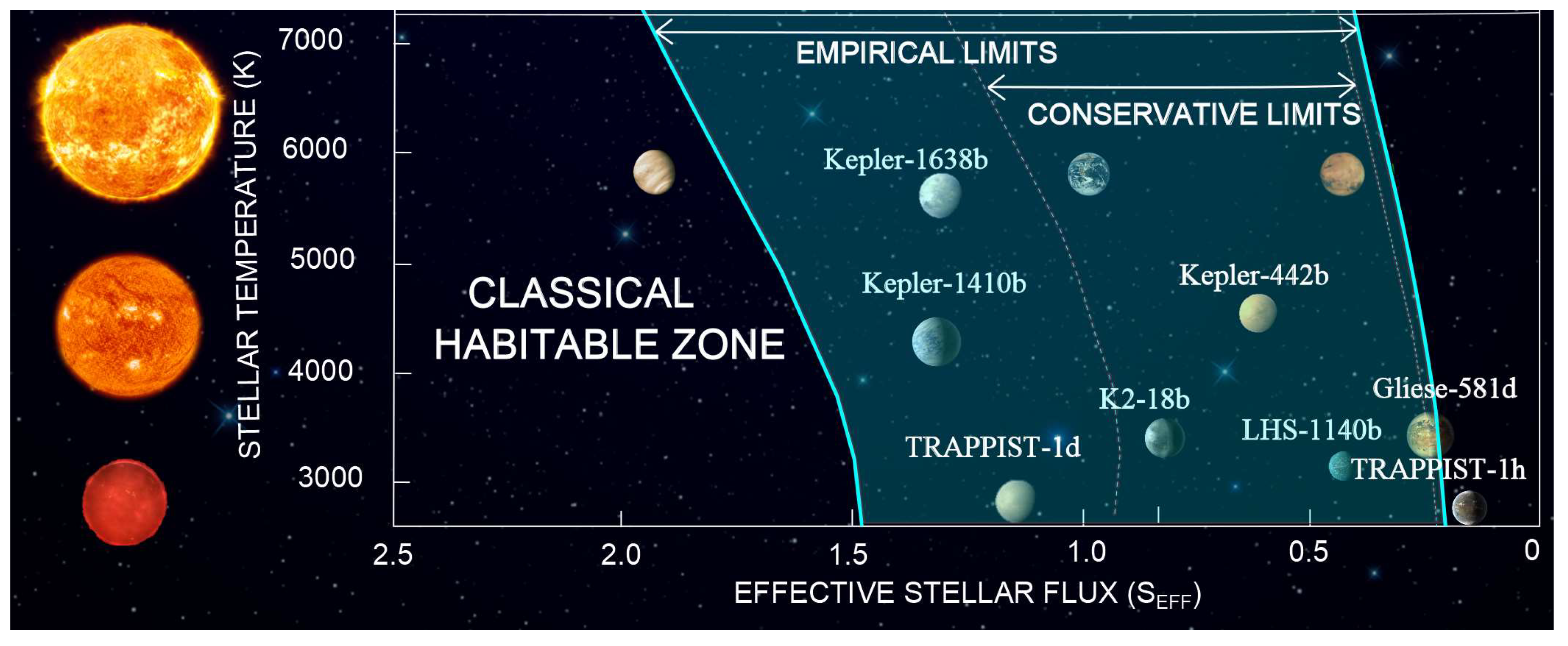
Figure 4.
Maximum surface temperature (black curve) and pCO2 level (green curve) for an Earth-like planet with a volcanic outgassing rate 10% of that of Earth’s orbiting a G-star (A) and F-star (B) for SEFF = 0.7. Transient periods of warming during which temperatures exceeding the freezing point of water (dashed line) are followed by extended periods of global glaciation (adapted from Haqq-Misra et al. [79]).
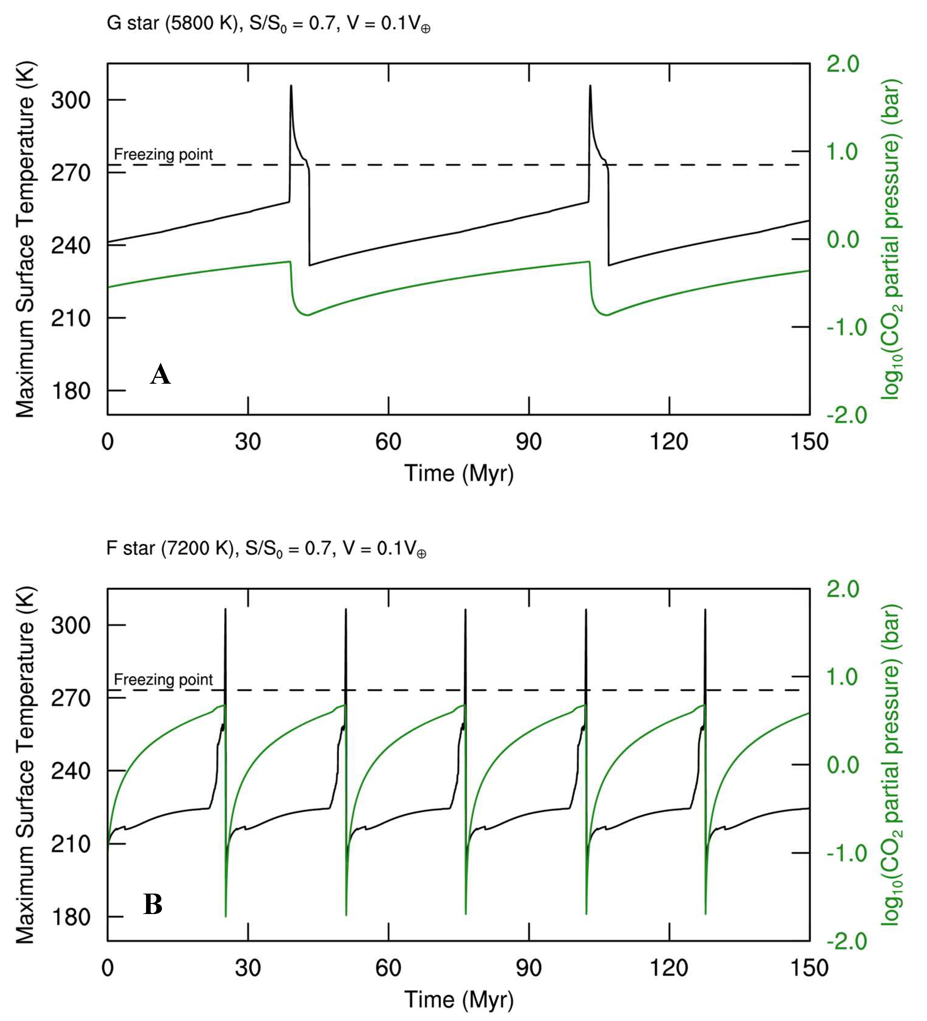
Figure 5.
Extended classical habitable zone for stellar temperatures from 2600 to 10,000 K (based on work from Ramirez and Kaltenegger [2]).
Figure 5.
Extended classical habitable zone for stellar temperatures from 2600 to 10,000 K (based on work from Ramirez and Kaltenegger [2]).
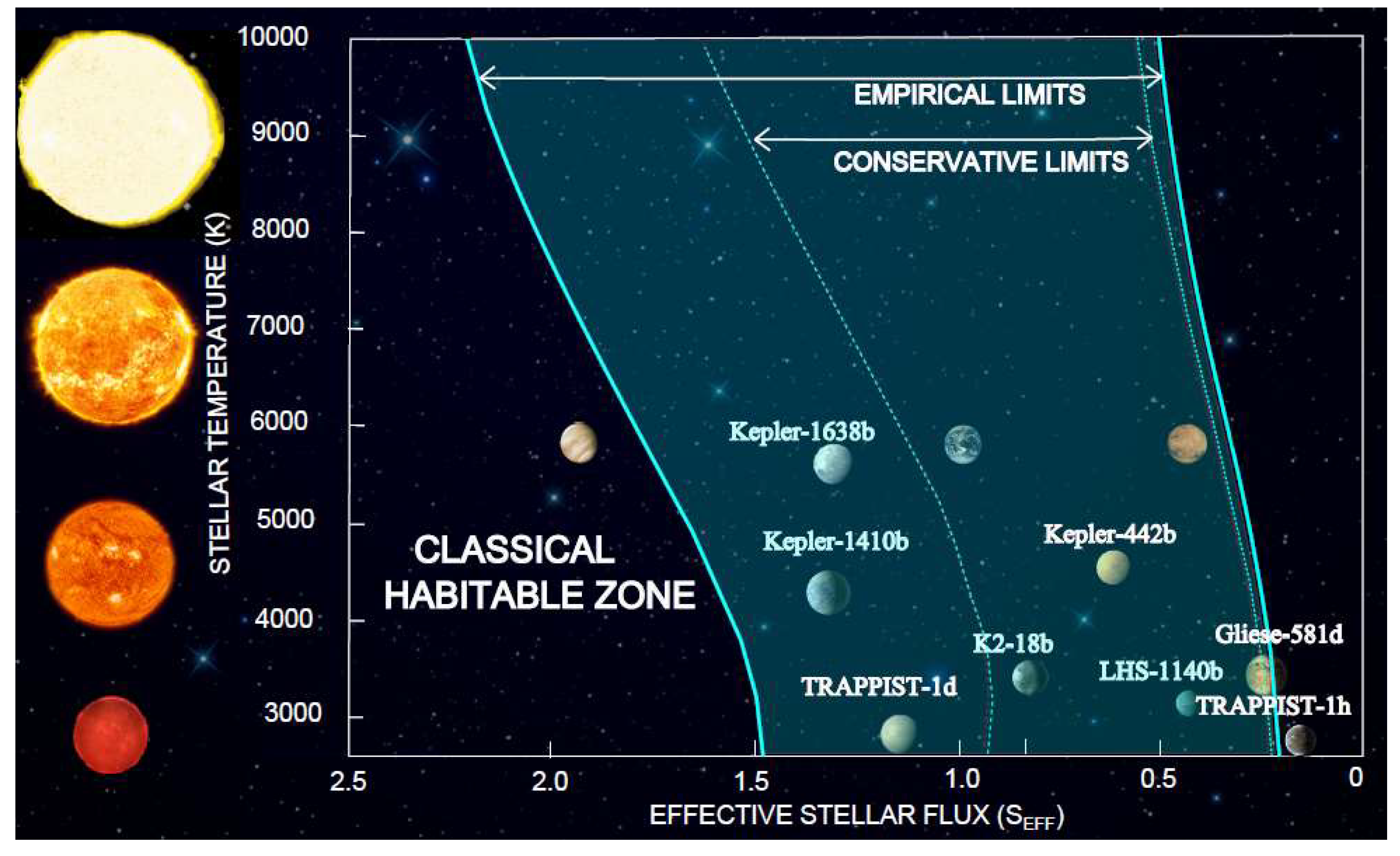
Figure 6.
Globally-averaged incoming stellar spectra for the Sun, F0, and M3 stars. Adapted from Ramirez and Kaltenegger [2] and updated from Ramirez [22].
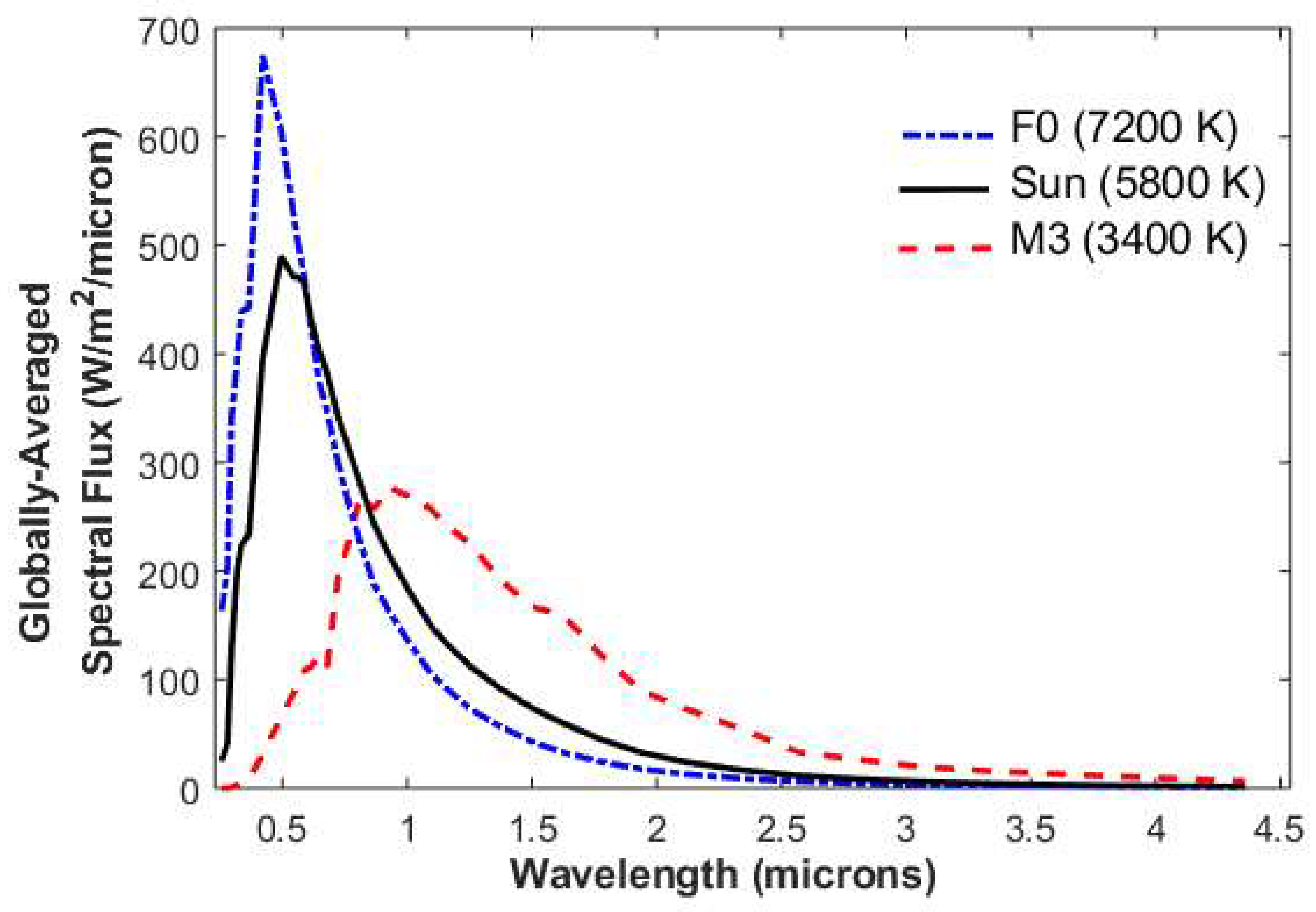
Figure 7.
Changes in temperature profiles for a 3-bar CO2 (1 bar N2) atmosphere (solar energy =33% that received by the Earth) for a model planet orbiting an F0 (blue) (A), (B) a G2 (black; solar-analog), and (C) an M3 (red) host star with and without 1% (10,000 ppm) CH4. A temperature inversion forms for all three planets. The surface temperature increases when CH4 is added on the planet orbiting the F0 (18 K) and solar (G2) analog (29 K), but decreases for the planet orbiting an M3 star (31 K). Adapted from Ramirez and Kaltenegger [2] and updated from Ramirez [22].


Figure 8.
The classical HZ (blue) with CO2–CH4 (green) and CO2–H2 (red) extensions for stars of stellar temperatures between 2600 and 10,000 K (A–M-stars). The same classical HZ boundaries shown in Figure 3 and Figure 5 are also shown. Some solar system planets and exoplanets are also shown. Based on work from Ramirez and Kaltenegger [2,131,132] and Ramirez [22].
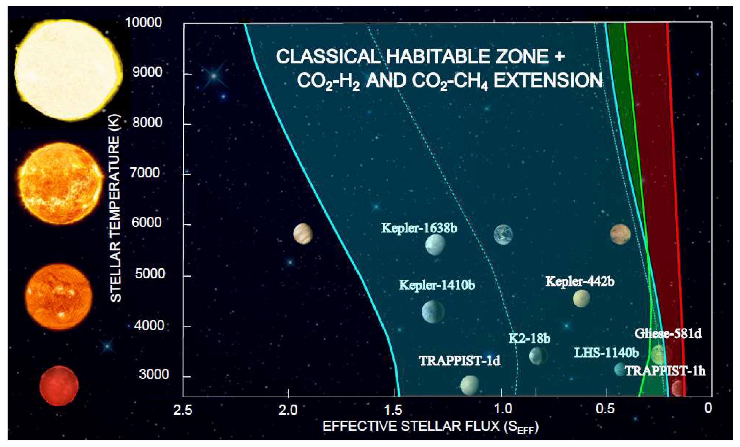
Figure 9.
Proposed “Daisyworld” scenario for planets at the outer edge of the methane HZ with CH4 in their atmospheres orbiting hotter (~A–G class) stars. The parabolic lines illustrate the effect that CH4/CO2 has on surface temperature, whereas the straight lines depict the effect of temperature on the CH4/CO2 ratio (figure adapted from Ramirez and Kaltenegger [2] and Domagal-Goldman et al.[173]).

Figure 10.
Evolution of stellar luminosity for F–M stars (F1, F5, Sun, K6, M1, M5, and M8) using Barrafe et al. [184] stellar evolutionary models. When the star reaches the main-sequence (red points) the luminosity curve flattens (updated from Ramirez and Kaltenegger [51]).

Figure 11.
The pre-main-sequence habitable zone for an M8. A planet originally located at 0.03 AU undergoes a runaway greenhouse for ~100 Myr before settling near the outer edge of the habitable zone at the start of the main-sequence. Based on work from Ramirez and Kaltenegger [51].
Figure 11.
The pre-main-sequence habitable zone for an M8. A planet originally located at 0.03 AU undergoes a runaway greenhouse for ~100 Myr before settling near the outer edge of the habitable zone at the start of the main-sequence. Based on work from Ramirez and Kaltenegger [51].

Figure 12.
Schematic of CO2 transport between ocean and atmosphere on ocean worlds. The ocean floor contains CO2 clathrate hydrates, while atmospheric winds drive an upper oceanic circulation that eventually degasses CO2 directly into the atmosphere (adapted from Ramirez and Levi [216]).
Figure 12.
Schematic of CO2 transport between ocean and atmosphere on ocean worlds. The ocean floor contains CO2 clathrate hydrates, while atmospheric winds drive an upper oceanic circulation that eventually degasses CO2 directly into the atmosphere (adapted from Ramirez and Levi [216]).

Figure 13.
Schematic of P-type (a) and S-type (b) binary star systems.

Figure 14.
Summary of recent 1D and 3D model estimates of the location of the inner edge for mid-K- to M-stars. The Leconte et al. [25] curve is the nominal inner edge estimate for rapidly-rotating planets, superseding the previous estimate [26]. The remaining limits are various 3D estimates for synchronously-rotating worlds.

Figure 15.
Sample flow chart using the classical HZ, along with CO2–H2, CO2–CH4, and pre-main-sequence HZ extensions to assess the potential habitability of planets. End states are in yellow.
Figure 15.
Sample flow chart using the classical HZ, along with CO2–H2, CO2–CH4, and pre-main-sequence HZ extensions to assess the potential habitability of planets. End states are in yellow.


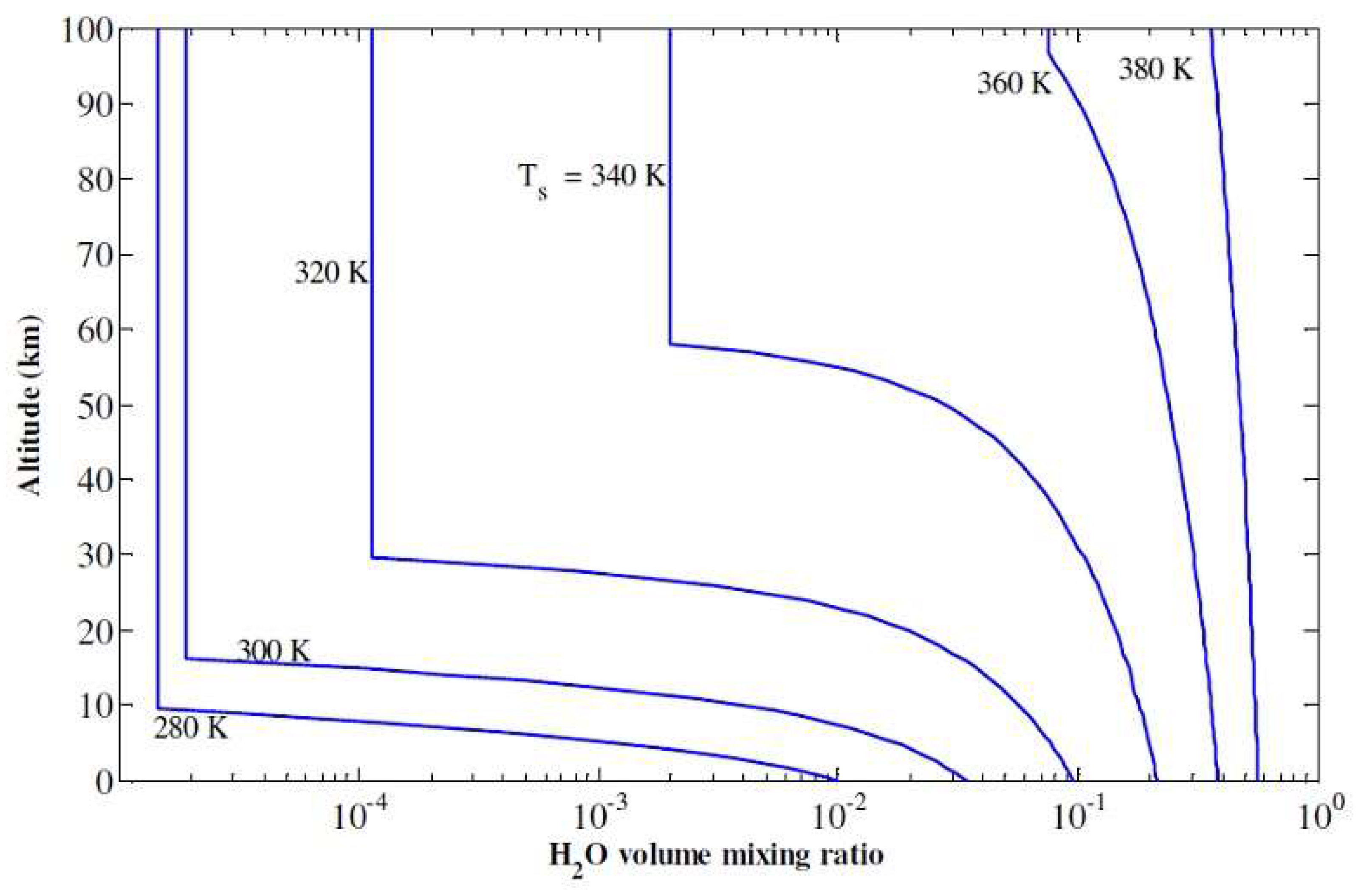
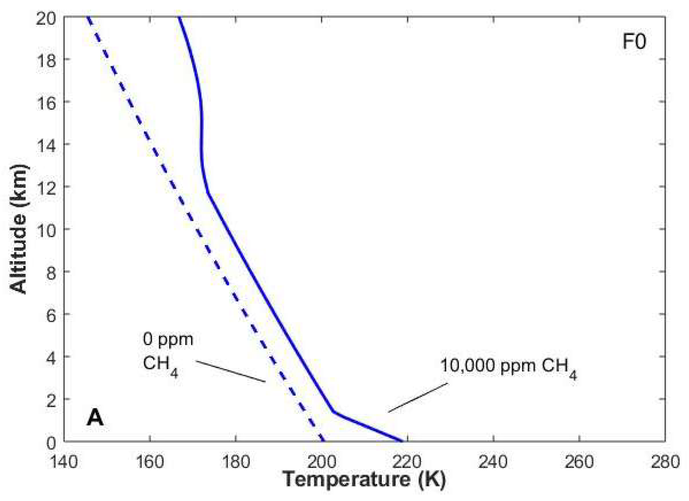
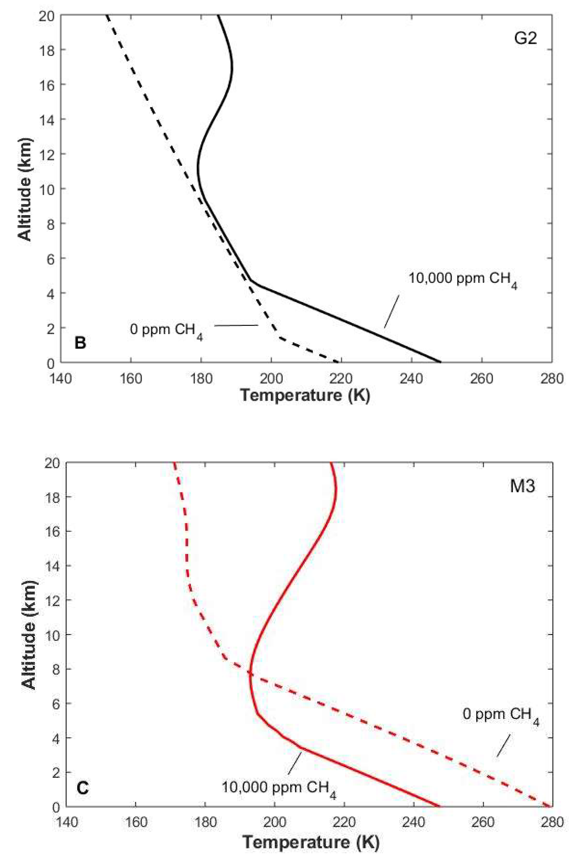
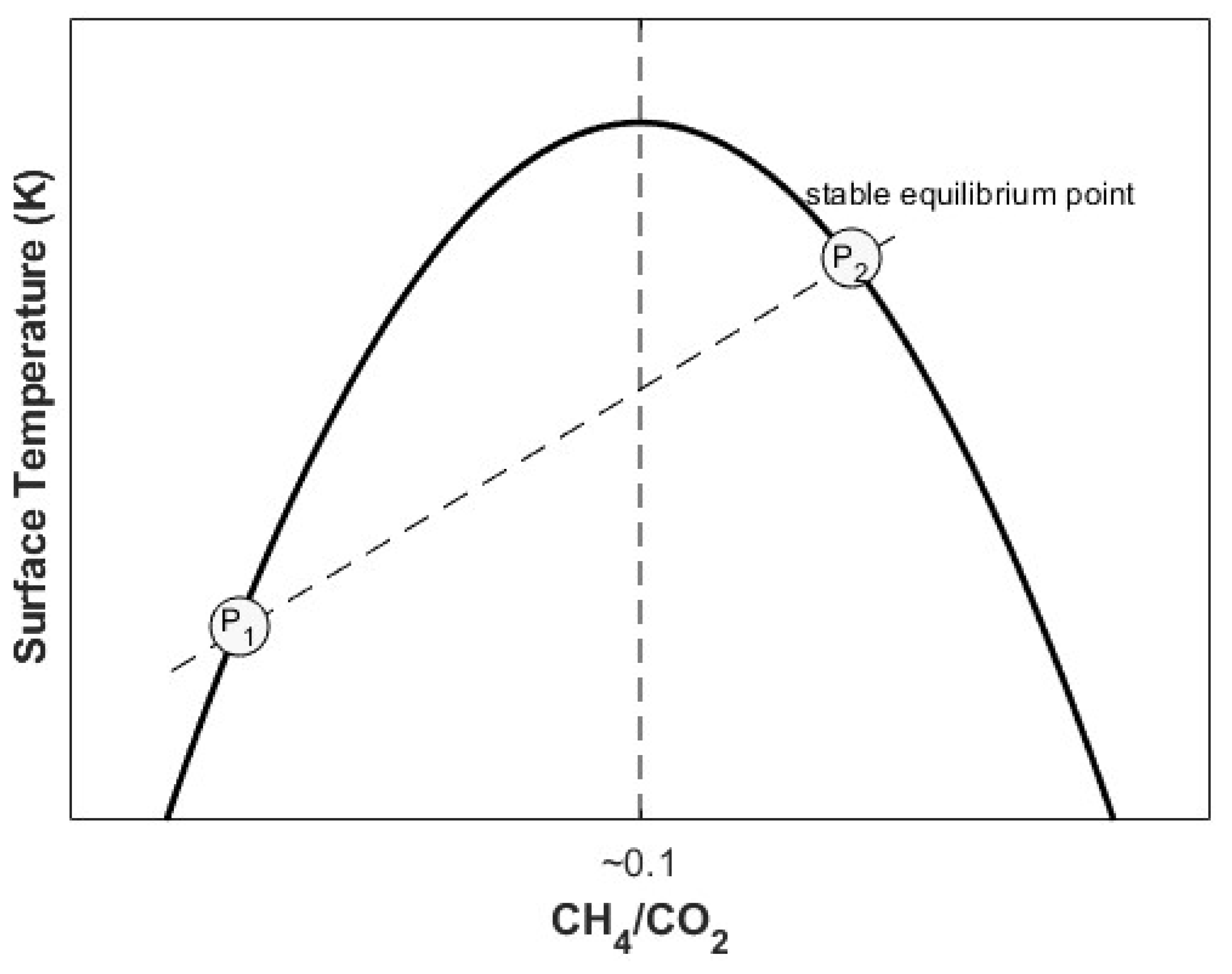
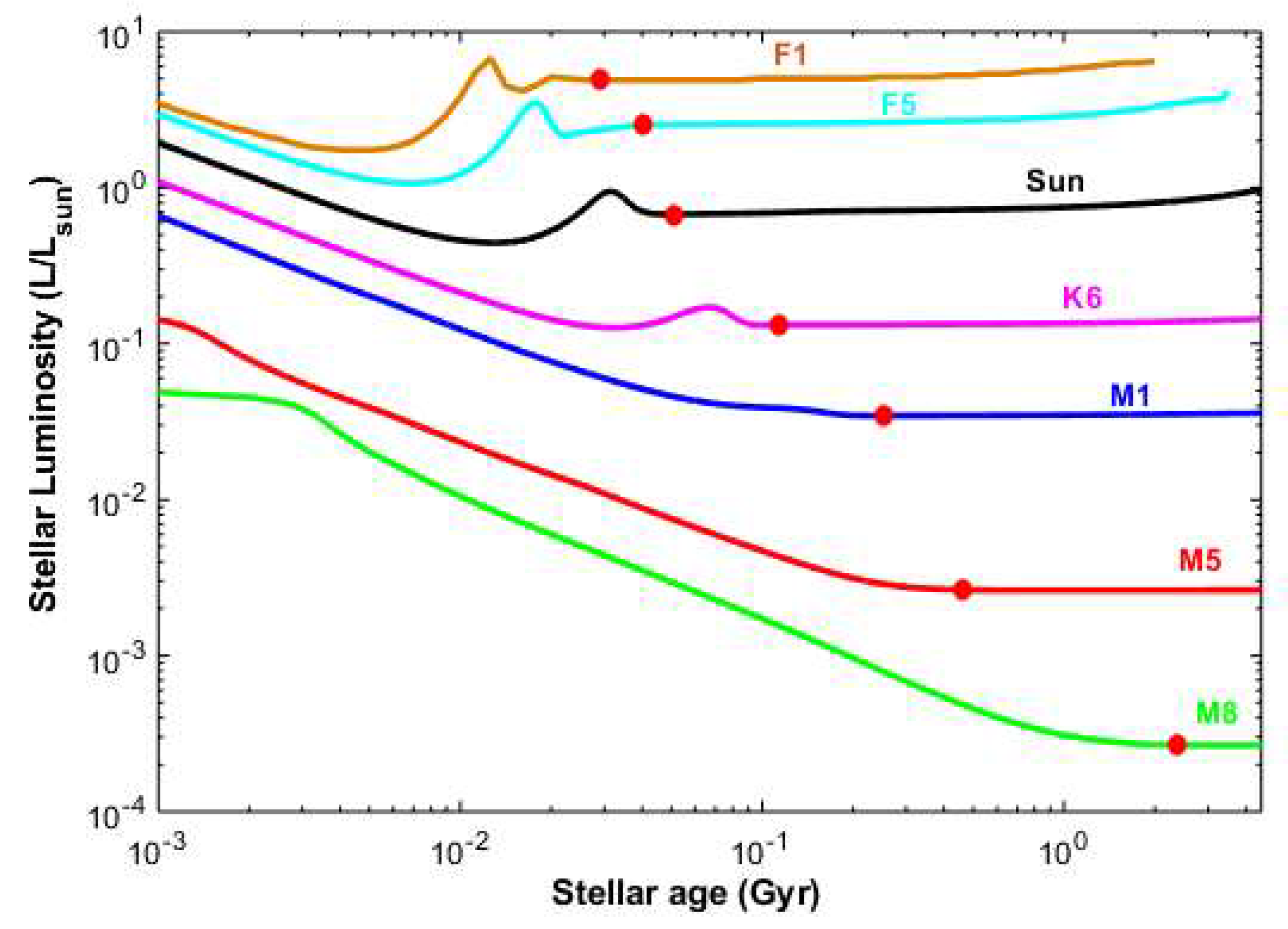
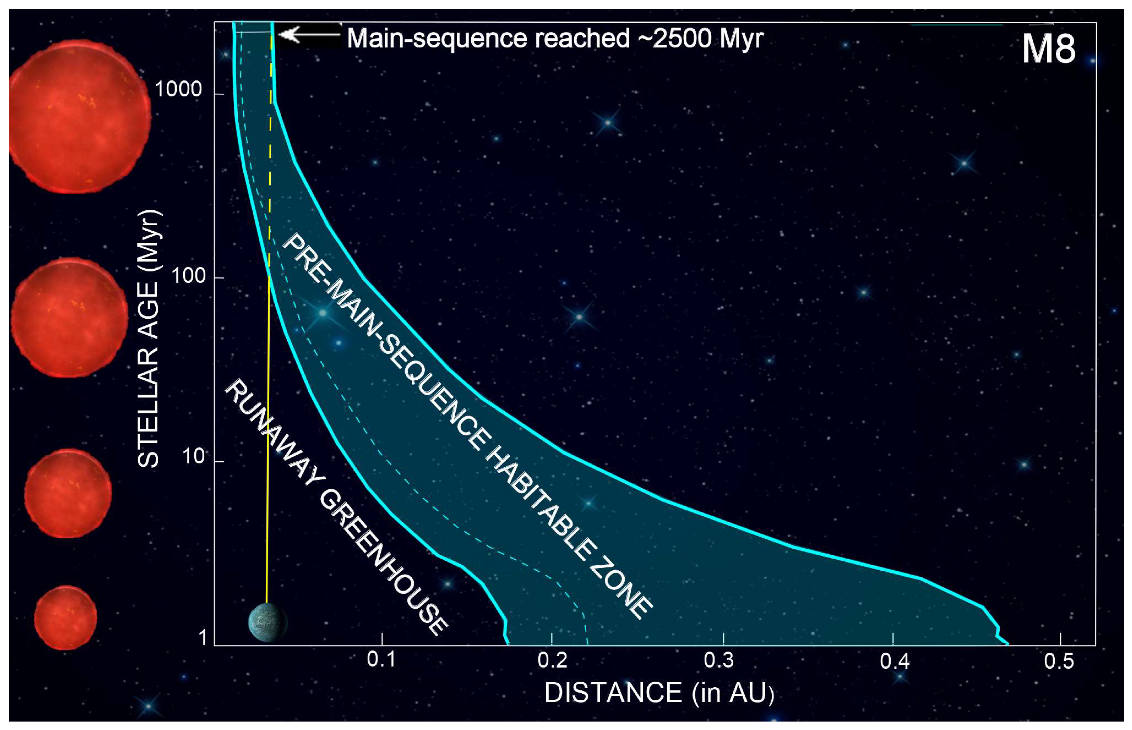
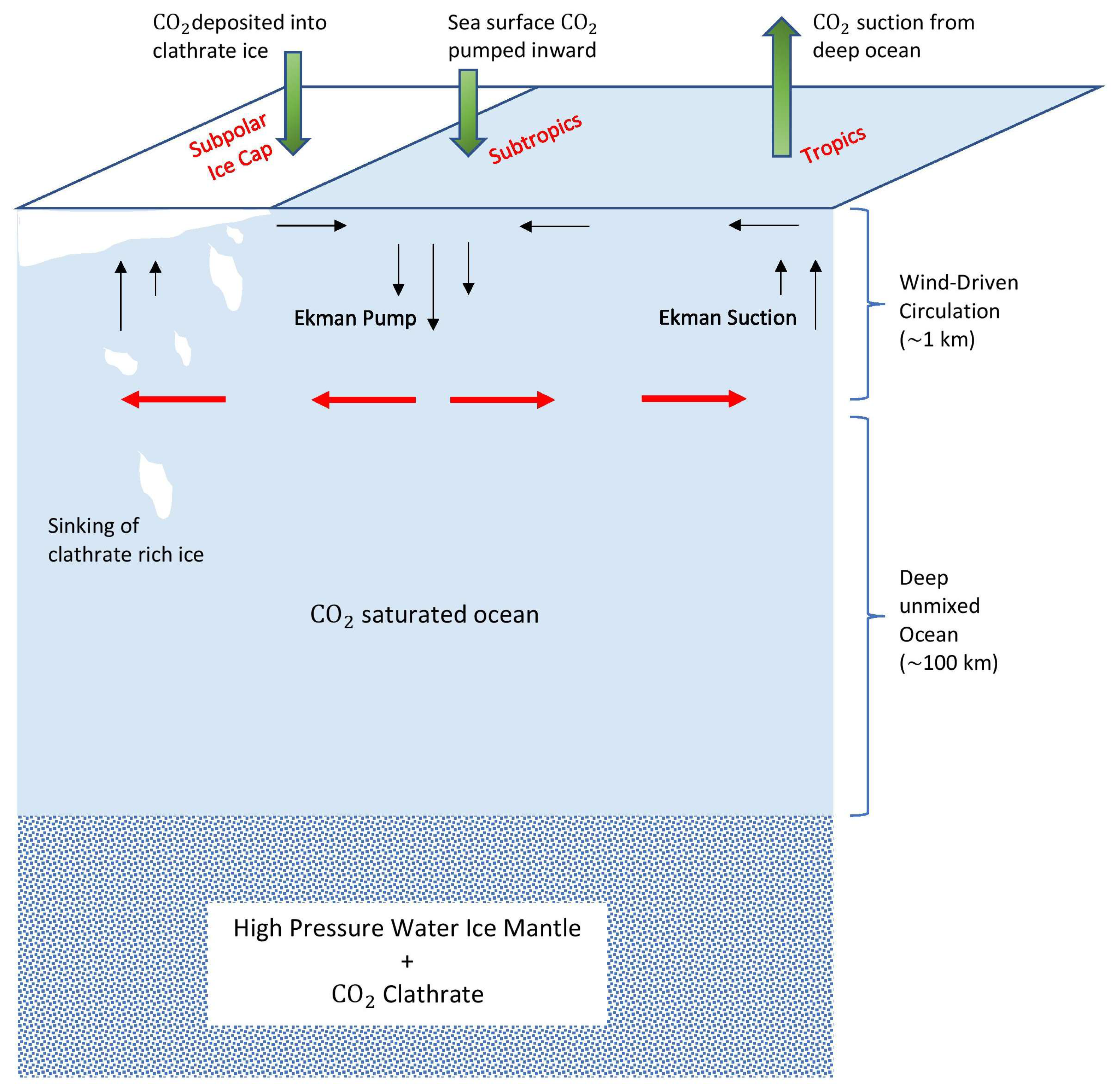
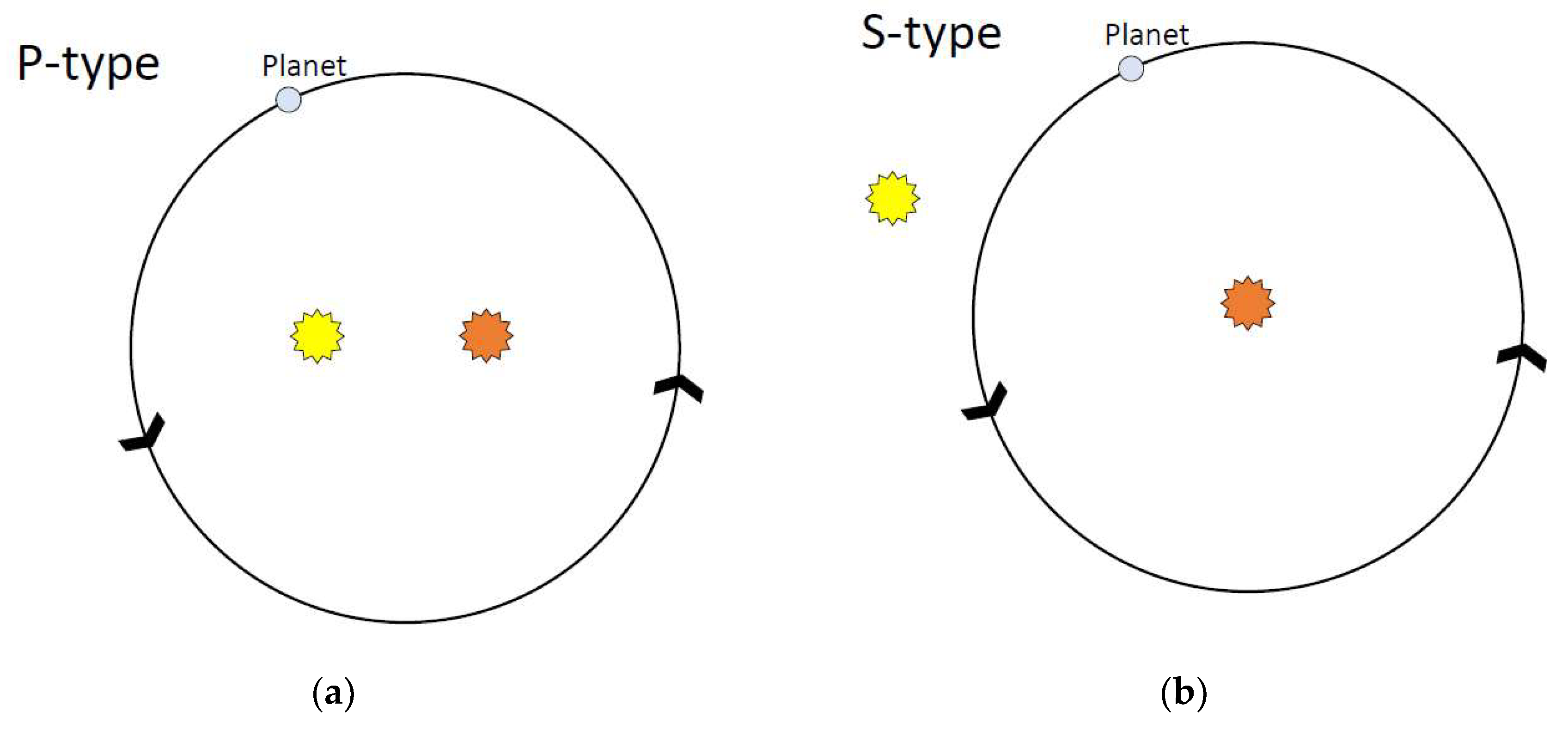
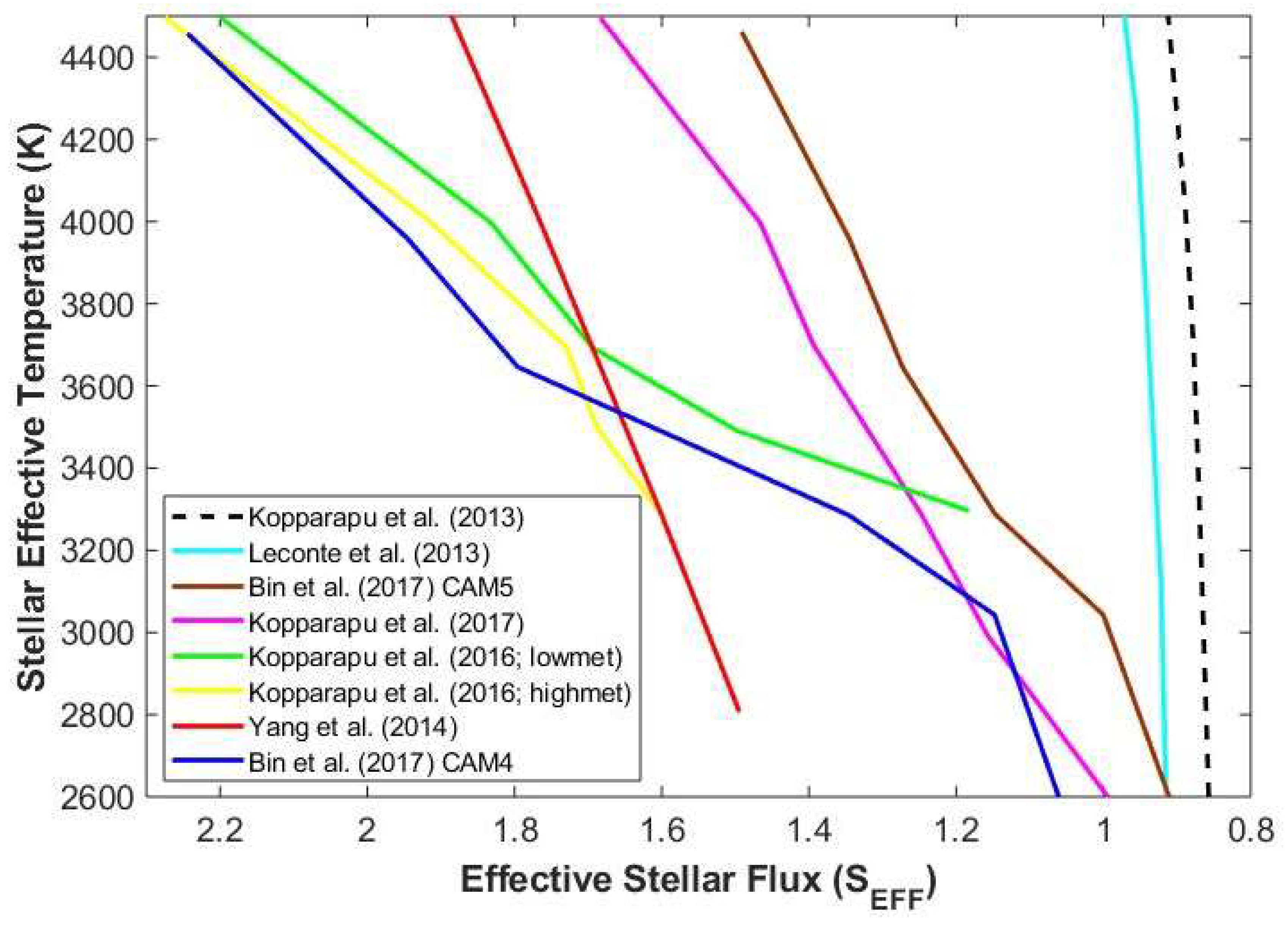
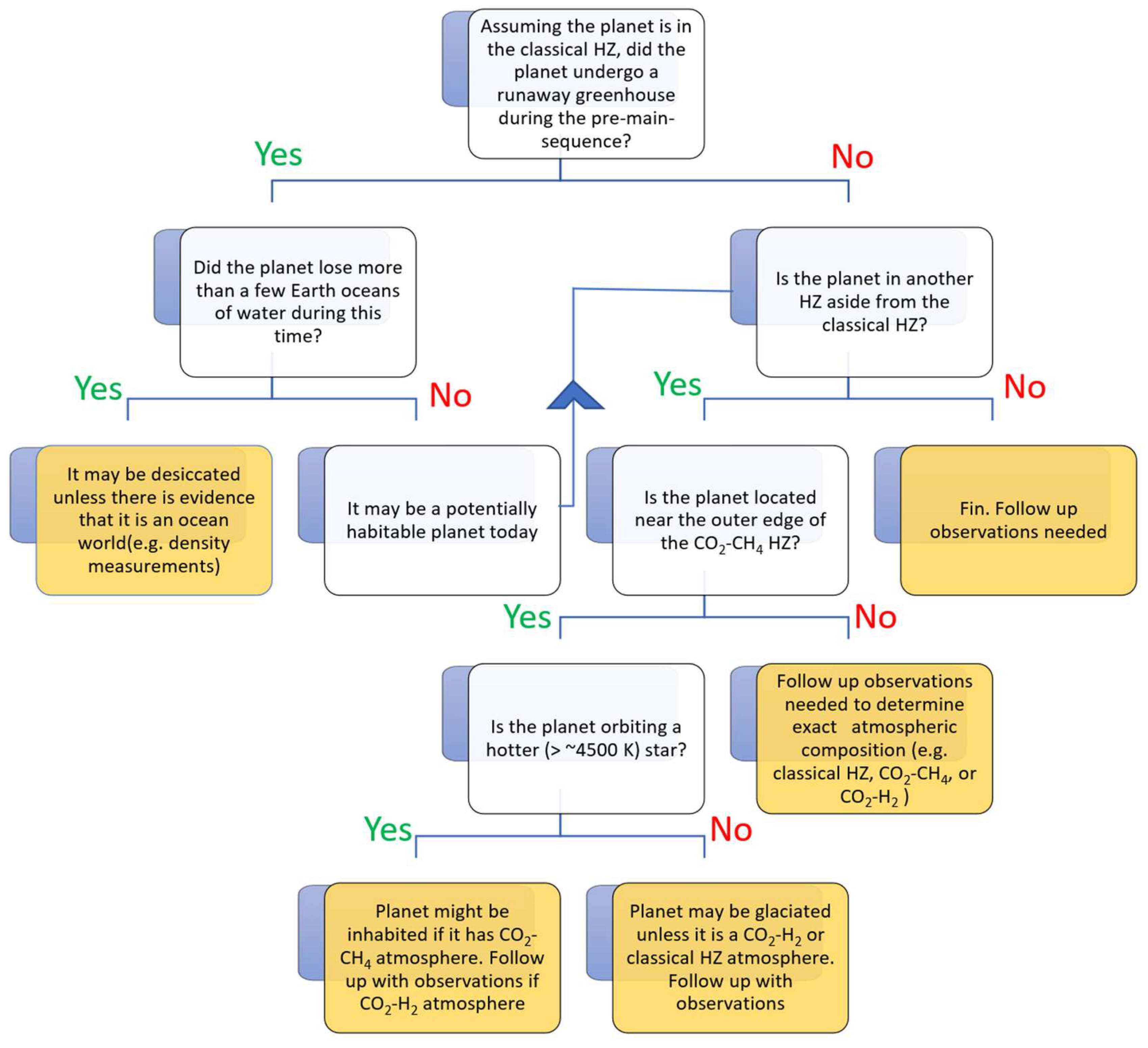
Table 1.
Revised coefficients for the extended classical habitable zone (HZ) (atmospheric composition N2-CO2-H2O) and the empirical HZ for host stars with TEFF = 2600–10,000 K *. SEFF—effective stellar flux.
Table 1.
Revised coefficients for the extended classical habitable zone (HZ) (atmospheric composition N2-CO2-H2O) and the empirical HZ for host stars with TEFF = 2600–10,000 K *. SEFF—effective stellar flux.
| Constant | Recent Venus | Leconte et al. | CO2 Maximum Greenhouse | Early Mars |
|---|---|---|---|---|
| SEFF(Sun) | 1.768 | 1.1105 | 0.3587 | 0.3246 |
| A | 1.3151 × 10⁻⁴ | 1.1921 × 10⁻⁴ | 5.8087 × 10⁻⁵ | 5.213 × 10⁻⁵ |
| B | 5.8695 × 10⁻¹⁰ | 9.5932 × 10⁻⁹ | 1.5393 × 10⁻⁹ | 4.5245 × 10⁻¹⁰ |
| C | −2.8895 × 10⁻¹² | −2.6189 × 10⁻¹² | −8.3547 × 10⁻¹³ | -1.0223 × 10⁻¹² |
| D | 3.2174 × 10⁻¹⁶ | 1.3710 × 10⁻¹⁶ | 1.0319 × 10⁻¹⁶ | 9.6376 × 10⁻¹⁷ |
* Reproduced from Ramirez and Kaltenegger [2] after fixing a typo.
© 2018 by the author. Licensee MDPI, Basel, Switzerland. This article is an open access article distributed under the terms and conditions of the Creative Commons Attribution (CC BY) license (http://creativecommons.org/licenses/by/4.0/).
Share and Cite
MDPI and ACS Style
Ramirez, R.M. A More Comprehensive Habitable Zone for Finding Life on Other Planets. Geosciences 2018, 8, 280. https://doi.org/10.3390/geosciences8080280
AMA Style
Ramirez RM. A More Comprehensive Habitable Zone for Finding Life on Other Planets. Geosciences. 2018; 8(8):280. https://doi.org/10.3390/geosciences8080280
Chicago/Turabian StyleRamirez, Ramses M. 2018. "A More Comprehensive Habitable Zone for Finding Life on Other Planets" Geosciences 8, no. 8: 280. https://doi.org/10.3390/geosciences8080280
Note that from the first issue of 2016, this journal uses article numbers instead of page numbers. See further details here.