Article

Site Effect Assessment of the Gros-Morne Hill Area in Port-au-Prince, Haiti, Part B: Mapping and Modelling Results

by
Sophia Ulysse
1,2,3,*,
Dominique Boisson
1,
Claude Prépetit
2 and
Hans-Balder Havenith
3,*
1
Research Unit in Geosciences, Université d’Etat d’Haïti, 6112 Port-au-Prince, Haïti
2
Bureau des Mines et de l’Energie, 2174 Port-au-Prince, Haïti
3
Department of Geology, Liège Université, 4000 Liège, Belgium
*
Authors to whom correspondence should be addressed.
Geosciences 2018, 8(7), 233; https://doi.org/10.3390/geosciences8070233
Submission received: 8 May 2018 / Revised: 14 June 2018 / Accepted: 14 June 2018 / Published: 23 June 2018

Abstract

:
This paper presents the general results in terms of maps, as well as geological and numerical models of a site effect study, that aimed at a better understanding of the ground motion amplification on the Gros-Morne hill, in the southeastern part of Port-au-Prince, Haiti, which might have influenced the 2010 event damage pattern in that area. These maps and models are based on multiple geophysical–seismological survey outputs that are presented, in detail, in Part A of this publication. Those outputs include electrical resistivity tomography sections, P-wave velocity profiles, S-wave logs, estimates of the fundamental resonance frequency for many locations, as well as earthquake recordings at three sites and associated site amplification assessment for the top of the hill. Related results are discussed in Part A with respect to outputs and interpretations that had been published earlier by other research teams for the same site. Our results only partly confirm the strong seismic amplification effects highlighted by some of the previous studies for this hill site, which had been attributed to the influence of local topographic and soil characteristics on seismic ground motion. Here, we focus on the imaging of different site effect components over the entire survey area; we present maps of shear wave velocity variations, of changing fundamental resonance frequencies, and of related estimates of soft soil/rock thickness, of peak spectral amplitudes, and of ambient ground motion polarization. Results have also been compiled within a 3D surface–subsurface model of the hill, which helps visualize the geological characteristics of the area, which are relevant for site effect analyses. From the 3D geomodel, we extracted one 2D geological section along the short-axis of the hill, crossing it near the location of Hotel Montana on top of the hill, which had been destroyed during the earthquake, and has now been rebuilt. This cross-section was used for dynamic numerical modelling of seismic ground motion, and for related site amplification calculation. The numerical results are compared with the site amplification characteristics that had been estimated from the ambient vibration measurements and the earthquake recordings.

1. Introduction

Haiti is crossed by several active faults that give rise to a substantial seismic hazard in Haiti ([1]), which can reach peak ground motion acceleration of 0.4 g for a 475-year return period in the vicinity of those faults. The last results by [2] show that this hazard level could even be higher than it had been predicted by [1] (see Figure 2 of Part A of this study presented in [3]).
The M = 7.1 Haiti earthquake on 12 January 2010, is the most recent expression of this high seismic hazard. Yet, the extent of the disaster caused by this event cannot purely be explained by those regional seismic hazard characteristics. In Part A of this study (presented in [3]), we refer to several elements that had already been highlighted soon after the earthquake as possible additional causes of the widespread destruction, such as the high building vulnerability and locally amplified ground motion ([4]).
Our study is focused on this latter effect, especially on site effects that might have contributed to more intense damage in the hilly areas in the southern part of Port-au-Prince, and in particular, on the hill of Gros-Morne (see location in Figure 1 below). For this site, several previous studies referred to possible site amplification in order to explain the severe damage in some zones on top of Gros-Morne hill, and along the southern slope caused by the 2010 main event, as evidenced by [5]. References [5,6,7,8] argue that local amplification effects are likely to have contributed to severe shaking and related destruction, such as the collapse of Hotel Montana on top of the hill (see location in Figure 1b); they attribute those effects both to topographical and soft soil amplification. In addition, reference [7] highlights the significant variability in soil response that is probably related to a complex subsurface structure.
The complex subsurface of Gros-Morne area is due its intermediate geological context, between the soft layers of the “Cul-de-sac Plain” in the north, and the hard rocks of the northern foot of the “Massif de la Selle” mountains in the south (see location in Figure 1 below). Along the ridge of the hill, both a soft (weakly compacted and locally weathered and marly) limestone, as well as calcareous breccia, are outcropping (see [3] for more detail). In some areas, even some clayey gravels can be found. The southwestern slope of the hill plunges towards the “Ravine Djobel”, that is occupied by a small river. At the bottom of this ravine, the soils are composed of marls, locally including small calcareous pebbles, as well as conglomeratic alluvia. Around Gros-Morne hill, the tectonic setting is marked by the presence of smaller active faults of middle to upper Quaternary age.

2. Geophysical Investigations

To determine the subsurface structure at the Gros-Morne site and assess the related local seismic response of soils, we completed an extensive geophysical–seismological survey. Results of this survey include five electrical resistivity and 16 seismic refraction profiles, 106 ambient vibration measurements, as well as earthquake recordings at three seismic stations during several months in 2017, and can be found in [3]. Below, we present a summary of the seismic and seismological survey outcomes that are considered as the most relevant inputs for the 3D geological and 2D numerical modelling study outlined in the fourth section of this paper.

2.1. Summary of the Ambient Vibration and Shear Wave Velocity Measurement Results

The single station ambient vibrations measurements were analyzed in terms of horizontal to vertical spectral ratios (HVSRs). These analyses first provide information on the local resonance frequencies; second, combined with shear wave velocity data, they allow us to assess the thickness of the amplifying layers. From the mobile single station measurements, we produced maps of the changing characteristics of the identified resonance frequency peak(s).
All ambient vibration measurements over the site were carried out with a maximum distance of about 350 m between two adjacent points. On the basis of the HVSR measurements, several ambient ground motion parameters have been mapped over the Gros-Morne hill: (i) the fundamental resonance frequency (f0), (ii) the amplitude of the main peak, and (iii) the corresponding polarization of shaking. In Figure 1 below, the locations of the selected representative HVSR recordings are shown with indication of the interpreted fundamental resonance frequency and the peak amplitude. Here, we consider the fundamental resonance frequency as the lowest frequency for which a relatively clear peak could be found. In some cases, also, some smaller peaks could be found below this frequency. A more detailed explanation of this map and the associated HVSR graphs can be found in Part A of this study [3]. Here, we focus on the use of the HVSR method for the mapping of site effect characteristics as presented below (Section 3), where we also discuss the possible origin of smaller low frequency peaks.
The seismic profiles (of a length up to 55 m) were mainly analyzed with the multichannel analysis of surface waves (MASW) technique. In particular, this method is used to determine the shear wave velocity parameter Vs30. By definition, Vs30 is the shear wave velocity averaged over the first 30 m of depth (considering a time-averaging procedure), and is commonly used in earthquake engineering for site characterization. In this regard, we are aware that the relatively short seismic profiles (with only 12 available geophones) do not allow us to entirely cover the first 30 m of soil. Due to the limited investigation depth, we defined a Vs15 parameter for each profile; this represents the average Vs value for the first 15 m (instead of 30 m, as indicated by the commonly used parameter Vs30). The lowest Vs15 values (<400 m/s) were measured along the lower parts of the hill, and especially in the south, at its base, within the ravine. The grounds along the ridge and the northeastern slope are marked by higher values (and are therefore considered to be more compact than at the rest of the study area). Along the hill ridge, the highest Vs values of up to 700 m/s were obtained at a depth of 10 m. By interpolating the results of all profiles, we created the map presented below in Figure 1b.

2.2. Earthquake Recordings

The earthquake recordings were acquired over a 63-day period in the beginning of 2017 with three accelerometers, which were respectively installed on the northern and southern slopes of the Gros-Morne hill (Delmas 60 and FIC), as well as on the top of the ridge (HM = Hotel Montana). The location of the seismic stations can be seen in the map in Figure 1b below. The amplification factor at the HM site was estimated with respect to the two other sites (Delmas 60 and FIC) by applying the standard spectral ratio (SSR) method. This ratio can be computed separately for all three components (two horizontal and the vertical components), but it can also be used by combining the average horizontal spectra. This method can be applied when the distance between the studied and the reference station is relatively small compared to the hypocentral distance of the earthquake, in order to assure similar characteristics of the incident wave fields for both stations. It should be noted that we could not find any ideal bedrock sites (marked by a flat hard rock surface, and ideally, by a bedrock with Vs30 larger than 1500 m/s) within the target area; therefore, we will consider a “relative SSR” for the HM site with respect to the two other sites that are actually not perfect reference sites.
The Geopsy software developed by [9] was used to visualize the seismograms and identify earthquake events. A total of 15 earthquakes were recorded at the three stations between 20 January and 23 March 2017. The events with an estimated epicentral distance higher than 50 km (practically all) were preselected for later processing. Then, the earthquakes with stronger amplitudes and larger signal length were chosen. Finally, only five events were selected to compute SSR (see characteristics in Table 1 of Part A of this study presented in [3]).
For each station and file containing a selected earthquake, HVSR graphs were computed both for ambient noise (HVSRN) and for S-waves of the earthquake recordings (HVSR_EQ). HVSR_EQ results for the Hotel Montana (HM) station are presented in Figure 2 below (where they are denoted S-waves HVSR), for the N–S, the E–W, and the combined components (see respective North, East, and average S-waves HVSR). For both horizontal components, and also for their squared average, the ratios essentially present two main amplified frequency ranges, one between 0.5 and 1.6 Hz and one between 2 and 4.5 Hz.
SSRs computed for HM-recordings with respect to Delmas 60 and FIC recordings are first determined separately for each horizontal component, E–W and N–S, as well as for each single earthquake. Then, an (arithmetic) average SSR for the five earthquakes is computed for each horizontal component. Finally, the squared average (Havg) of the horizontal components is calculated (as the squared average was also used for the HVSR and HVSR_EQ ratios for the combination of the horizontal components; a review of combination types of horizontal component spectra is provided by [10]; see also [11], supporting the use of quadratic mean that is equivalent to the squared average for average spectral ratio calculations). The resulting SSR are compared with the S-waves HVSR (squared average for both E–W and N–S components) in Figure 2a,b. The Figure 2a1,a2, respectively, present the E–W and N–S SSR using station FIC as reference. E–W and N–S SSR using Delmas 60 as reference station are shown in the Figure 2b1,b2, respectively.
Relatively low to medium amplification factors are outlined by the SSR computed with respect to both reference sites. The highest amplification factors vary between two and three. The peaks observed for the SSR computed with respect to Delmas 60 recordings are around 2–2.5 Hz, 4 Hz, and 7.5 Hz, while those observed for the SSR calculated with respect to FIC are between 0.5 and 2 Hz.
The standard spectral ratios using both FIC and Delmas 60 as reference stations allow us to confirm two resonance frequency peaks, i.e., the first around 0.5–1.6 Hz and the second of smaller amplitude around 2.5–4 Hz, identified from the S-waves HVSR measurements.
In [3], we also discuss which of those peaks could be attributed to possible topographic effects on Gros-Morne hill. In particular, it can be observed that between 1–2 Hz, the N–S SSRs show for both reference stations larger amplitudes than the E–W SSRs. This could be due to the preferred N–S vibration of the entire roughly WNW–ESE oriented hill, which is, thus, subparallel to the NNE–SSW oriented short axis of the hill. Topographic amplification is generally marked by such a polarization of the wave field, with stronger amplitudes perpendicular to the main axis (i.e., along the short axis) of the hill or mountain (see, e.g., overview on topographic effects in [12]). This N–S polarization is one argument that we use to attribute the low 0.5–2 Hz peak(s) to topographic effects related to the resonance of the hill as a whole. Other influences of local morphologies (slope breaks, slope orientation changes) and a more detailed analysis of the various types of site effects will be presented in the next section, also with the support of numerical modelling results.

3. Site Effect Analysis

3.1. Site Effect Distribution Maps

Site effect characteristic maps of the study area are presented in 
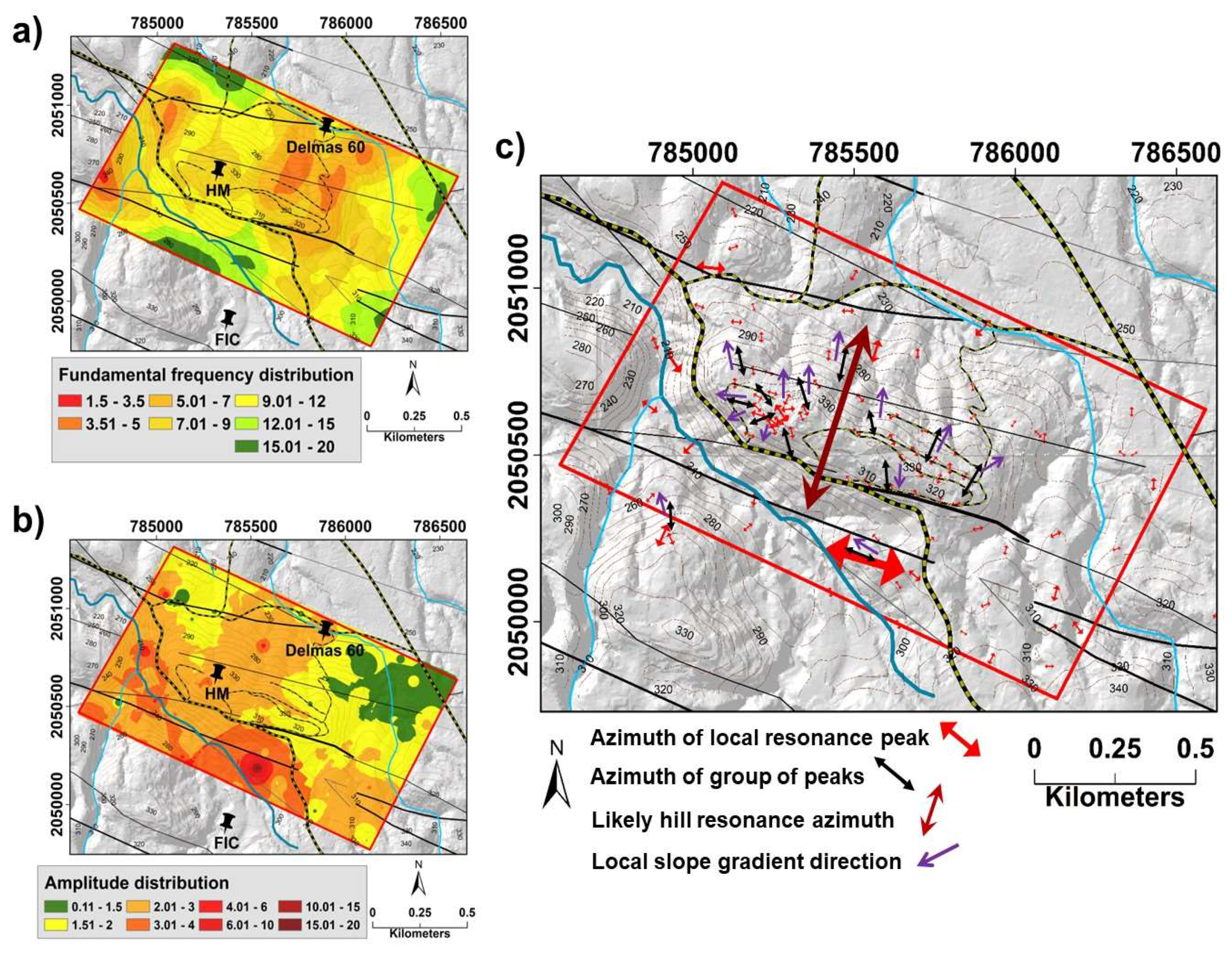
Figure 3. As a preliminary approach to seismic microzonation of the target area, we first interpolated the values, respectively, of the HVSR fundamental resonance frequencies (of the clearest low-frequency peak) and of the related peak amplitudes (related maps are presented in Figure 3a,b below). An overview map of the ground motion polarization at the identified resonance peaks is shown in Figure 3c; the preferential shaking orientation is represented by a red double-arrow (with size proportional to the peak amplitude averaged for both horizontal components). It can be seen that those polarizations are quite variable over the hill; only those in the north and south of the central part of the hill are roughly parallel to the short axis of the morphological structure (marked by the large brown double arrow in the map in Figure 3c below). To get a clearer overview on this phenomenon, we also plotted black double-arrows on that map to represent the polarization of resonance motion for a group of measurements. If we compare the black double-arrows with the local slope gradient direction (marked by violet arrows in the same map), we can see that they are preferentially parallel to them. Thus, it can be concluded that the polarization of the ground motion at the identified resonance frequencies is rather influenced by the local slope orientation than by the one of the hill as a whole (especially near the western and eastern end of the hill). Actually, all identified HVSR peaks along the top parts of Gros-Morne hill occur at frequencies clearly higher (>3 Hz) than the likely hill resonance frequency that would be between 0.5 and 2 Hz (inferred from the SSR presented above). Those peaks are, therefore, most likely caused by soft layer ground motion resonance rather than by the hill shaking resonance. Nevertheless, with an azimuth generally parallel to the slope gradient, these peaks seem to be marked by a slight and more local morphological effect as well.
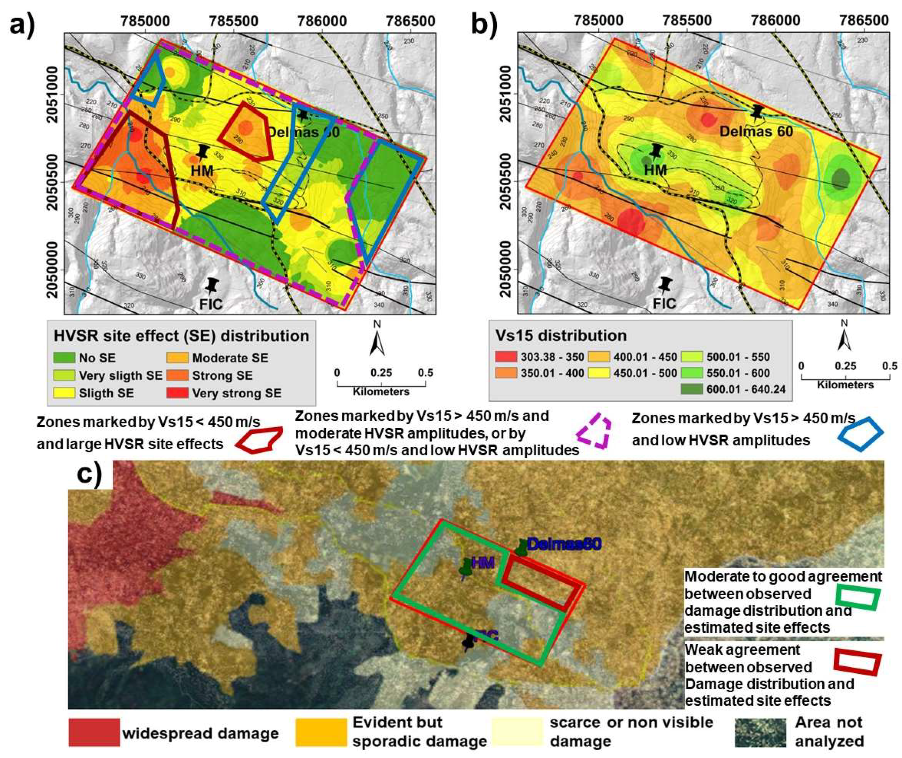
The two first maps (of interpolated resonance frequencies and peak amplitudes) have been combined to provide a map of site effect intensity (included in Figure 4). Areas with stronger site effects are considered to be characterized, first, by higher HVSR peak amplitudes (>3) and, second, by fundamental resonance frequencies relevant for earthquake engineering purposes (below 9 Hz). Zones marked by a combination of those characteristics are filled by orange to red colors in the HVSR site effect distribution map in Figure 4a; such zones can be found in two main areas around the Gros-Morne hill, a larger zone in the west, and a smaller one in the north of the hill. The Hotel Montana is located in an intermediate zone characterized by moderate estimated site effects with HVSR amplitudes that can reach values of 3, at frequencies between 5 and 12 Hz. It should be noted that the combined information does not consider topographic effects (at lower frequencies), but only site effects potentially resulting from soil amplification.
In 
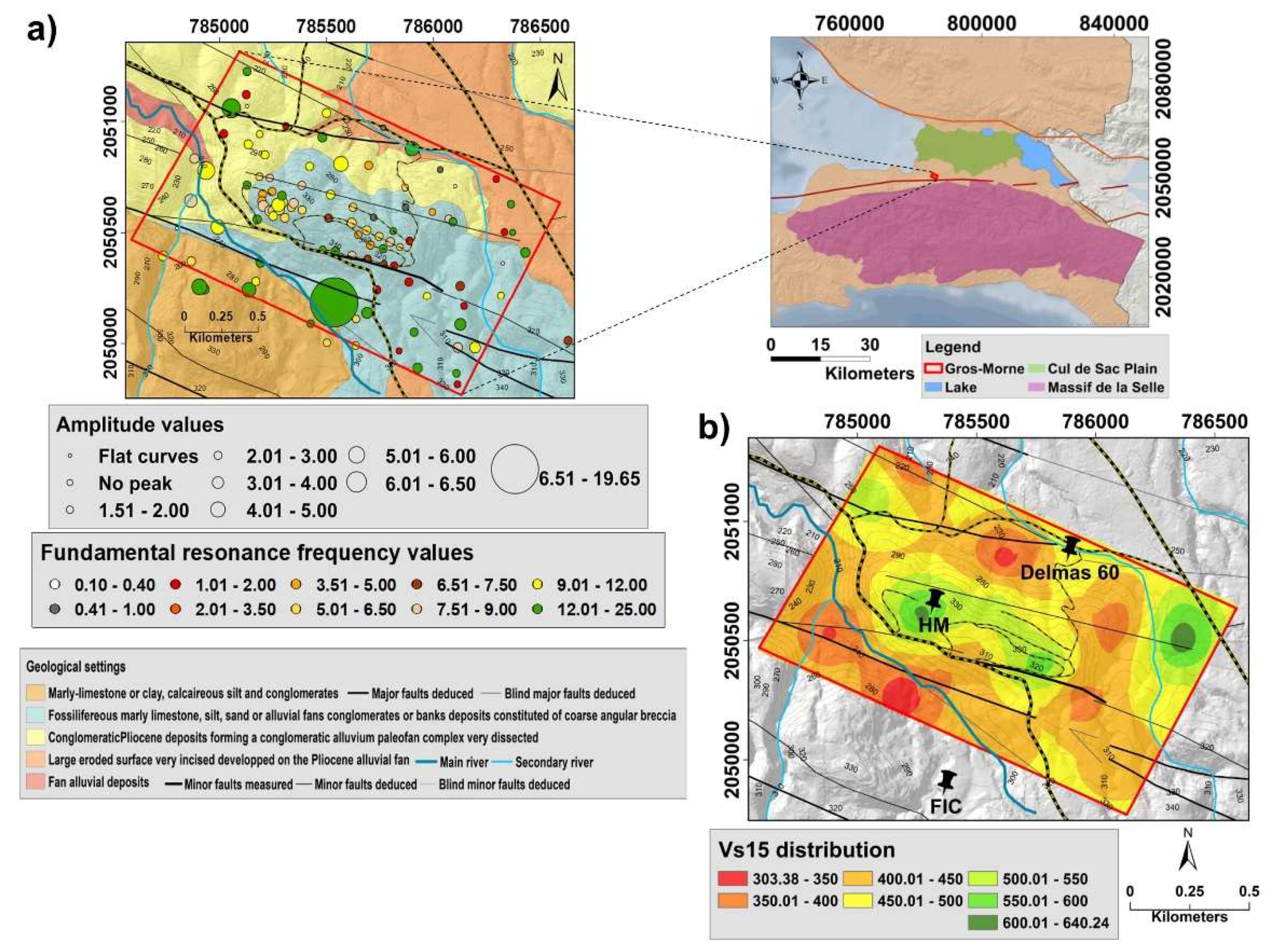
Figure 4, the “HVSR site effect” map (Figure 4a) is compared with the Vs15 map (Figure 4b) that has already been introduced above. It can be observed that areas marked by larger “HVSR site effects” present highly variable Vs15 values. Along the ridge where relatively large Vs15 values have been measured, both low and moderate to locally strong “HVSR site effects” can be found. In the southwest, zones are characterized by both low Vs15 values and medium-strong site effects. The northeastern corner, near the road Route de Delmas, seems to be the least prone to soil amplification with high velocities similar to those measured at Hotel Montana, but marked by weak “HVSR site effects”. Comparing the maps of the Vs15 values and “HVSR site effects” with an extract of the 2010 damage distribution map (Figure 4c) produced by [13], two main zones can be identified: the first zone in the west and south presents a moderate to good agreement between observed damage distribution and estimated site effects (with green outline in Figure 4c), while the second zone in the northeast presents a weak agreement between observed damage distribution and estimated site effects. The first zone includes two types of areas: for two areas in the northwest and south, lower site effects have been estimated, and scarcer damage had been observed while we assessed larger site effects for the central area, where, indeed, more extensive building destruction was evident. According to our estimates of site effects, the northeastern zone (district of Delmas) should not be exposed to strong ground motion amplification; nevertheless, it was affected by widespread damage.

3.2. Geophysical–Seismological Results Used to Build a 3D Geomodel

The thickness of the amplifying surface layers covering the hill was assessed and mapped on the basis of the joined HVSR and MASW results. Therefore, we used the resonance frequency peaks of the HVSR noise curves to compute the thickness of the different layers by applying the 1D assumption relation f0 = Vs/4h. The Vs parameter considered here is the average shear wave velocity obtained from the MASW measurements for the first 15 m (Vs15-value introduced above). Given that the relation f0 = Vs/4h is only applicable in the case of a soft layer overlying hard rock (or any denser layer), it was exclusively used for recordings showing a clear (sharp) resonance peak (amplitude ≥ 2). For locations marked by flat-shaped HVSR curves, it can be assumed that no very soft layer is present near the surface. At those sites, only the seismic data were used to estimate the subsurface structure. The validity of this approach is analyzed in the Discussion section below.
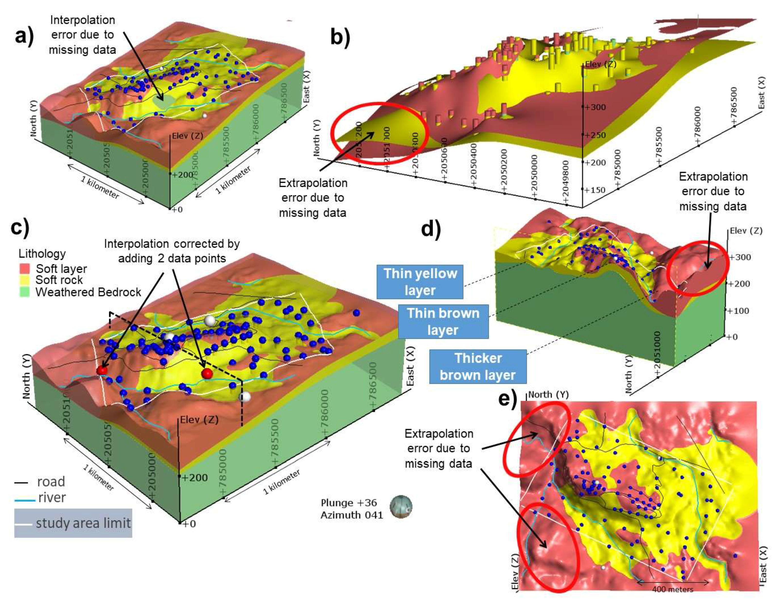
The low-velocity layer thickness values estimated by the above method were combined with the surface data to build a 3D geomodel of the Gros-Morne hill by using the Leapfrog Geosoftware (developed by ARANZ GEO, Christchurch, New Zealand). The resulting 3D geomodel presented in Figure 5 can be considered as a preliminary result as only geophysical data have been used to construct the subsurface; at the time of model construction, no borehole data were available (see also Discussion below).
The geomodel basically consists of two layers: the bedrock (green volume, see Figure 5) and the soft rock (yellow layer) that produces the fundamental resonance frequency peak. However, as a second frequency peak (and sometimes even a third one which is not considered here) was also observed for many investigated sites, the soft layer was regionally split into a shallow low-velocity (discontinuous shallow brown layer) and an intermediate layer (continuous yellow layer on top of the entire bedrock volume); the brown low-velocity layer is only present in zones marked by the occurrence of a second clear resonance peak, except for the northwestern corner, where it defines a single thick layer. Actually, the continuous yellow layer basis crosses the brown layer basis near the northwestern corner, due to extrapolation problems in this part of the model (see zone marked by the red ellipse in Figure 5b); yet, this does not modify the total thickness of the soft layer and the zone is located mostly outside the investigation area. The thickness of these near-surface layers (both the brown and the yellow layers) was computed by applying the aforementioned relationship h = Vs15/4f, with f representing the identified resonance frequency. The computed thicknesses of the shallow sedimentary layers vary between 5 and 27 m. Therefore, we considered that the maximum study depth is 30 m, and consequently placed the lower limit of the logs H/V at this depth (this depth has no effect on the model itself, that was purely built by interpolating surface topography and layer contact points). In this regard, a first source of error can be highlighted, the one of the probable underestimated thickness for sites where the computed layer thickness is clearly larger than 15 m, as the equivalent average shear wave velocity is likely to be larger than the Vs15-value that was used for thickness calculation. The logs, representing the thickness of the combined second and (where present) of the third layer, are represented by log-bars in Figure 5b.
From 106 HVSR recordings and 16 MASW measurements, a first model was computed, as explained above. In order to get the shear wave velocity values at each HVSR recording point, we used the nearest value indicated by the Vs15 distribution map shown in Figure 4b. However, as observed in Figure 5a, the first model also produced some interpolation errors due to data sparsity, notably for areas where we could not make any recordings during the field survey (partly due to inaccessibility of sites located on steep slopes of the hill). In order to have a better distribution of the frequency values to model the amplifying layers, two HVSR depth logs were added to areas with missing measurements; those added depth logs take into account the frequency and the velocity values, and consequently, the thickness values calculated for the surrounding HVSR sites; they were needed as, due to the changing topography in the sparse data areas, the interpolated surfaces crossed each other (and crossed also the topographic surface, similar to the extrapolation problem highlighted above, for crossing the yellow basis surface by the brown layer basis in the northwestern corner; note, an additional extrapolation problem appears in the western part of the model where the brown surface layer becomes very thick—but this appears mainly outside our target area). In the Figure 5c below, we show the final model with the measured HVSR logs (blue points) and the added ones (red points). The white points are the seismic stations plotted on the model. The other views (Figure 5d,e) respectively show an E–W section, as well as a map-view of the model.
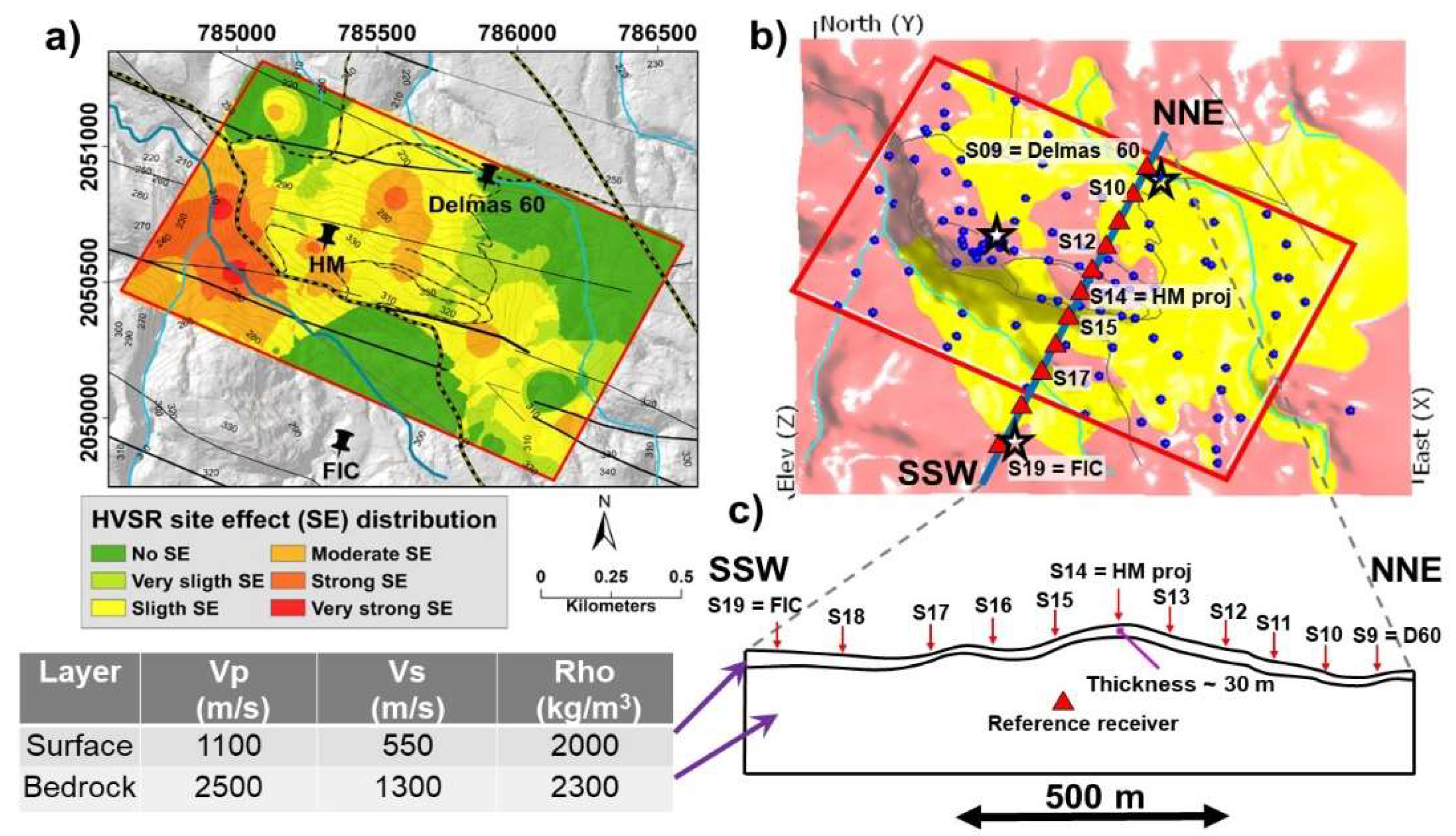
The map-view of the resulting geomodel presented above in Figure 5e is also compared with the HVSR site effect distribution map in Figure 6. This comparison shows that the shallow brown and yellow layers roughly correspond to, respectively, the orange to red, and the yellow to green areas of the HVSR site effects map. Thus, in the geomodel, the shallow yellow layer is related to areas marked by a weak to moderate potential of site amplification, while the brown layer outlines zones where moderate to strong site effects can be expected. Areas with the strongest soil amplification potential are distinguished from those with moderate site effects by their greater thickness. Indeed, from a north–south section view in Figure 5d, it can be seen that these low velocity layers (<400 m/s) are thicker in the southwestern foothill and very thin on the hilltop. Likewise, moderate site effect areas can be outlined by means of the thickness of the yellow layer. In the northeastern corner, where weak site effects have been identified, the yellow layer is thinner, while it is thicker on the slope going to the ridge. It is important to note that among the three seismic stations, only the Delmas 60 one is located in an area where the brown layer is not present.
From the 3D geomodel, a 2D section with simplified geology was extracted (shown in Figure 6c); it includes a surface layer marked by P-wave (Vp) and S-wave (Vs) velocities, and a volumic mass that were averaged over the entire layer, as well as a bedrock with estimated average elastic properties marked by Vs of 1300 m/s (see table in Figure 6). The estimates of elastic properties for the bedrock are based on data published by [14], which have also been discussed in [3]. This 2D section presented in Figure 6c was used for elastic dynamic simulations that are presented in the next Section 3.3.

3.3. Simple 2D Numerical Models of the Target Site

In order to better understand the observed amplification effects on and near the Gros-Morne hill, dynamic numerical modelling was performed. The tool applied for those simulations is based on the distinct element method (DEM) which is a numerical solution used to describe the mechanical behavior of discontinuous bodies. The latter are systems composed of discrete elements or blocks (here, the layers marked by different elastic properties) separated by interfaces (here, the layer boundaries). Introduced by [15], the DEM was developed for the analysis of rock mechanics and was later implemented in the 2D UDEC software (Universal Distinct Element Code, Itasca consulting group). The UDEC software actually combines the DEM with the finite difference method (FDM), determining the deformation of the material inside a block, which allows for a more general application of the tool. In particular, the latter component is essential for the simulations carried out for the Gros-Morne site as the compliance of the rock matrix is of relevance in the considered problem; therefore, each block (here, the surface layer and the bedrock) can be subdivided into zones to enable internal deformation computed by FDM. The main advantage of subdividing the medium into distinct elements is to allow the system to evolve further than a continuous FD or FE continuum, and to enable singular blocks to deform separately. However, in the present case, the singular block deformation option was not used, and the model was constructed as a continuum, and this by “gluing” the contact (by setting very high joint cohesion values) between the surface layer and the bedrock. It should be noted that we modelled only in the elastic domain; to simulate the effect of energy dissipation (such as through viscous attenuation), the implemented Rayleigh damping scheme was applied (see explanation, e.g., in [16]); along the boundaries, free field conditions were included.
The 2D numerical calculations were applied to the NNE–SSW section extracted from the 3D geomodel of the hill (Figure 6), which is perpendicular to its main axis of elongation, and extends from the FIC to the Delmas 60 sites. The section is 1230 m long, and reaches a maximal elevation of 333 m on top of the Gros-Morne hill. The section initially includes three main elements deduced from the 3D model: the two surface layers and the basement (bedrock). For the simulations, this structure has been simplified, and only one single surface layer with average elastic properties was included (simplification was applied as this is a preliminary study that will be more developed within a future project). Amplification effects can, therefore, only vary along the model surface, due to the changing layer thickness (depending on the local measured HVSR fundamental frequencies that were used to construct the 3D geomodel), and due to the local topography. For both the surface layer and the bedrock material, the bulk and the shear moduli (K and G), as well as the volumic mass had to be defined, the two first on the basis of the Vp- and Vs-values determined for those layers (see elastic properties in the table in Figure 6). Also, the response of a pure topographic model has been simulated; in this model, the surface layer characteristics are the same as for the bedrock.
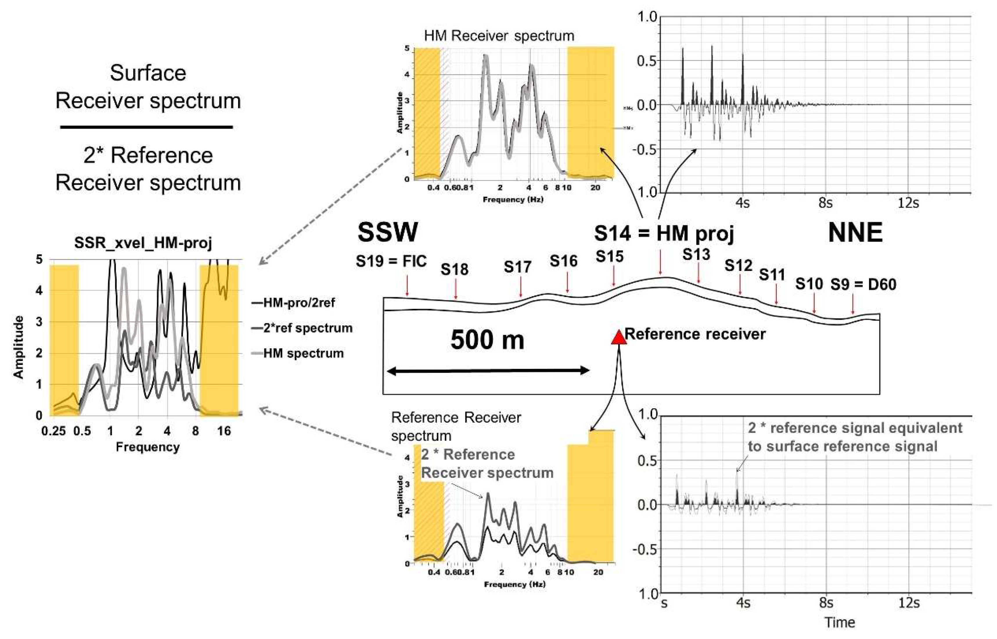
Along the surface of the model, eleven surface receivers have been inserted; additionally, one subsurface receiver was included in the middle of the model at a depth of about 120 m. The configuration of the model and receiver locations is shown above in Figure 6c, as well as in Figure 7. At the basis of the model, three successive Ricker wavelets marked by two central frequencies at 1.5 and 4 Hz (with main vibration in the x or the horizontal direction) have been introduced, and propagated upward across the model. The signal recorded at the reference receiver and the corresponding spectrum, as well as the doubled spectrum, supposed to represent the one of a surface receiver on bedrock, are shown in the lower part of Figure 7 (there, see also the dashed signal with doubled amplitudes). An example of signal and corresponding frequency spectrum recorded on top of the Gros-Morne hill (at receiver S14 representing a site equivalent to the one of Hotel Montana) is shown in the upper part of Figure 7. The standard spectral ratios (SSRs, see left part of Figure 7) were computed for the eleven surface receivers by dividing the respective surface receiver spectrum by the doubled subsurface reference receiver spectrum. Parts of the input signal spectrum that do not include sufficient energy (and are not considered for analysis) are masked by an orange semi-transparent rectangle in all figures below.
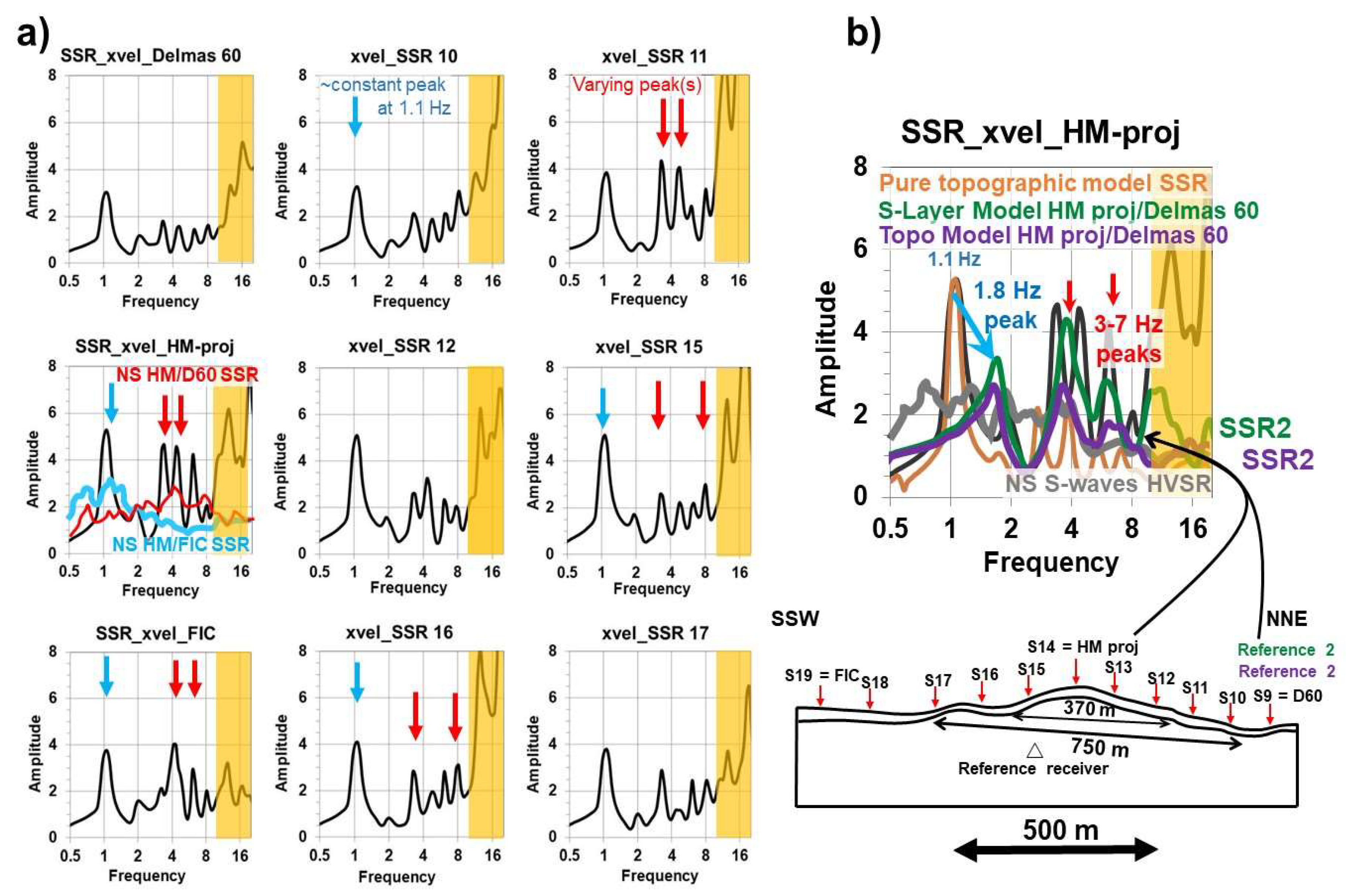
SSRs are presented for nine surface receivers in 
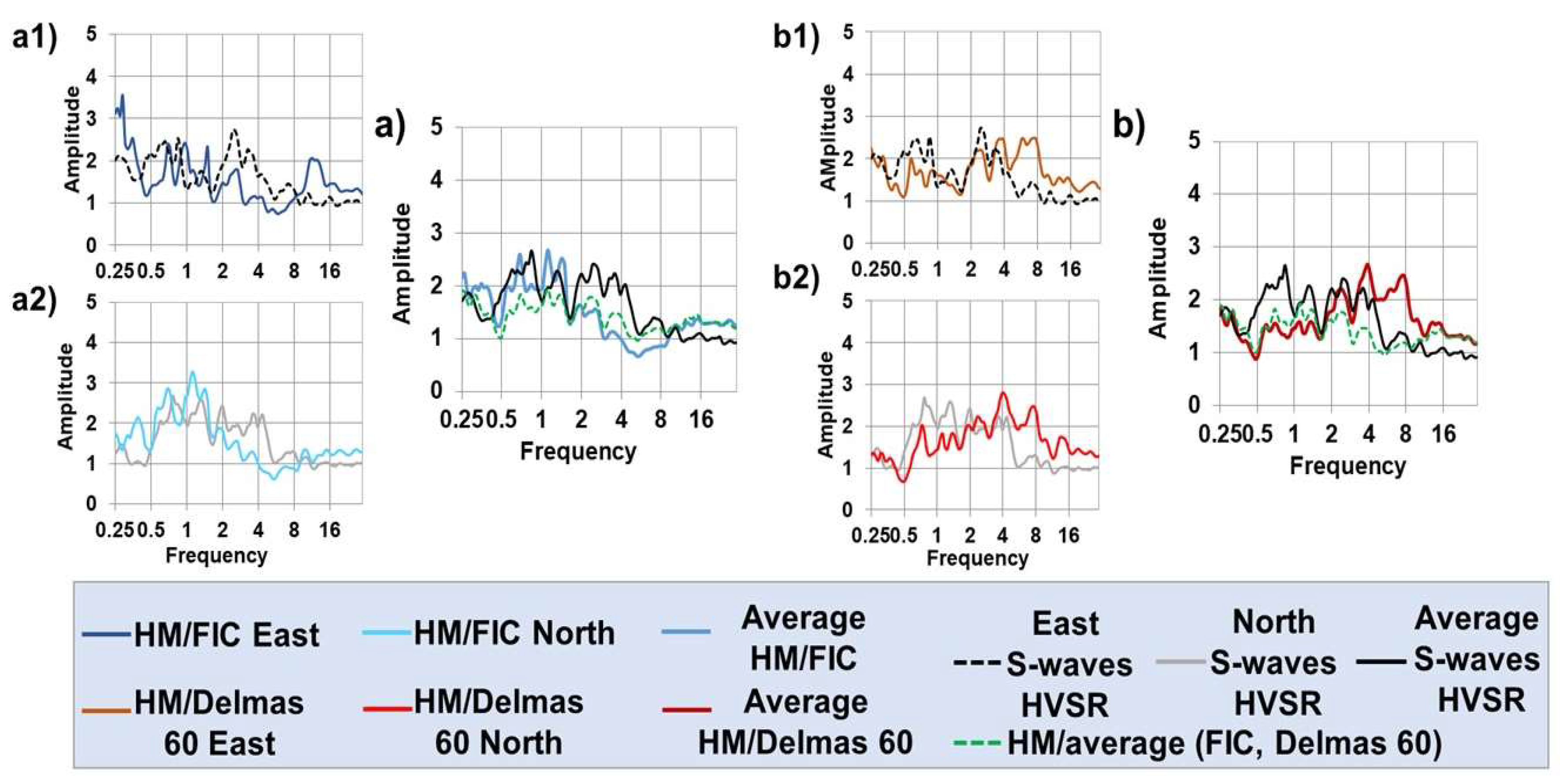
Figure 8 (with the high frequency part masked due to insufficient energy in the input signal). For the equivalent HM receiver S14 (middle left part of 
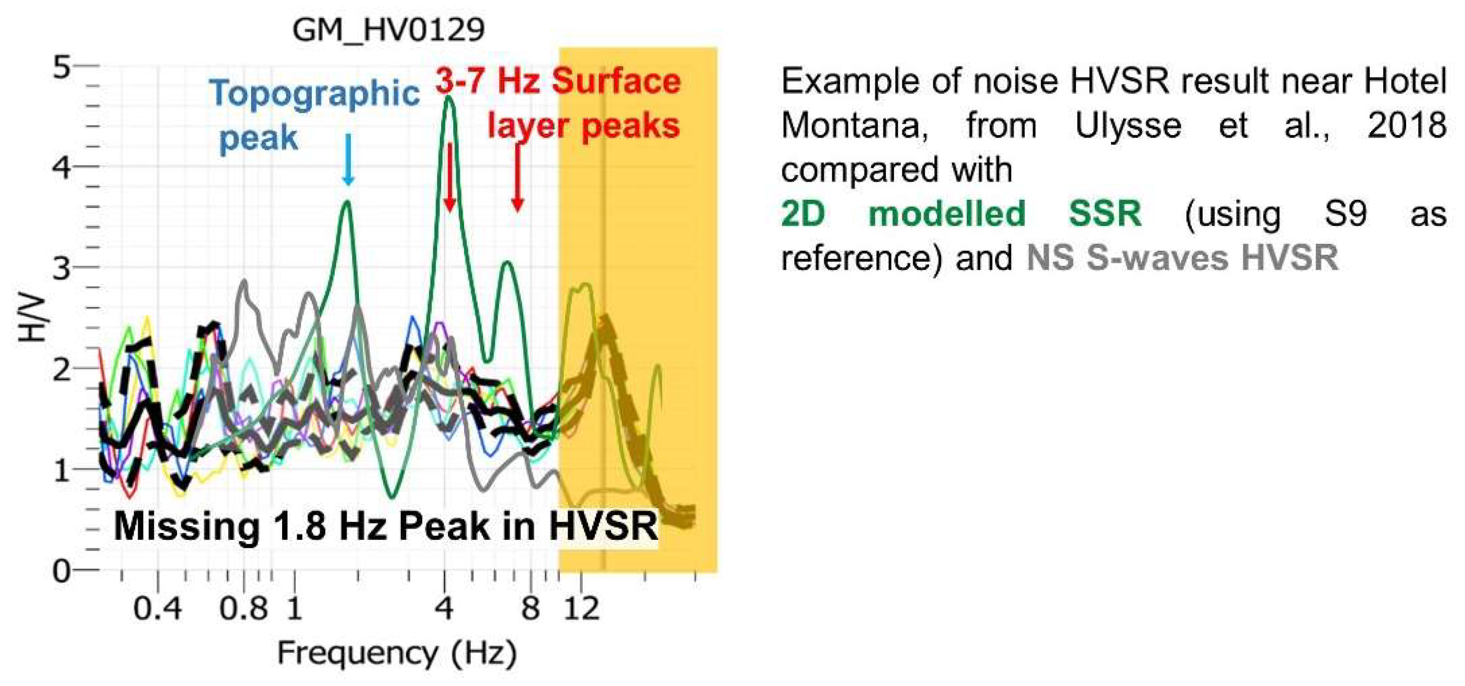
Figure 8a), the modelled SSR is compared with the measured NS SSR obtained with respect to FIC station (in blue) and to Delmas 60 station (in red). The same modelled SSR is enlarged and compared in Figure 8b, with the NS S-waves HVSR (in grey) and with the SSR obtained for the equivalent location in the purely topographic model (in beige, with surface layer characteristics identical to those of the bedrock, marked by Vs = 1300 m/s). This comparison shows that the first peak at 1 Hz is produced both by the purely topographic model and by the model including a softer surface layer (with Vs = 550 m/s). The results in Figure 8a show that this first peak is present at all sites, but changes in amplitude, the smallest one (~2.8) was obtained for the low-altitude site in the NNE part of the section, and the highest one (~5.3) for the receiver near the hill top (representing the equivalent HM site). The SSR obtained for the hill top in the purely topographic models also presents smaller peaks at higher frequencies. It should be noted that at similar frequencies, the model with a soft surface layer produces clearly larger amplifications. The combined measured NS SSR computed with respect to FIC and Delmas 60 station shown in Figure 8a and the NS S-waves HVSR, altogether, present several moderate peaks between 0.5 and 9 Hz; from the comparison with the modelled SSRs for the hilltop site (for both the purely topographic model and the one with a surface layer), it can be inferred that the low frequency peak around 1 Hz is likely to be due to topographic amplification, and those above 2 Hz are probably related to surface layer site effects.
However, the size of the ‘”topographic” peak (amplitude > 5) is surprising, as topographic amplification is generally limited to factors of 2–3. Actually, in the field, topographic amplification is almost exclusively assessed with respect to other surface receivers, especially those located at the foot of the hill or mountain structure. Here, the SSRs were computed with respect to a subsurface receiver that is located at a great depth well below the basis of the hill. Therefore, in 
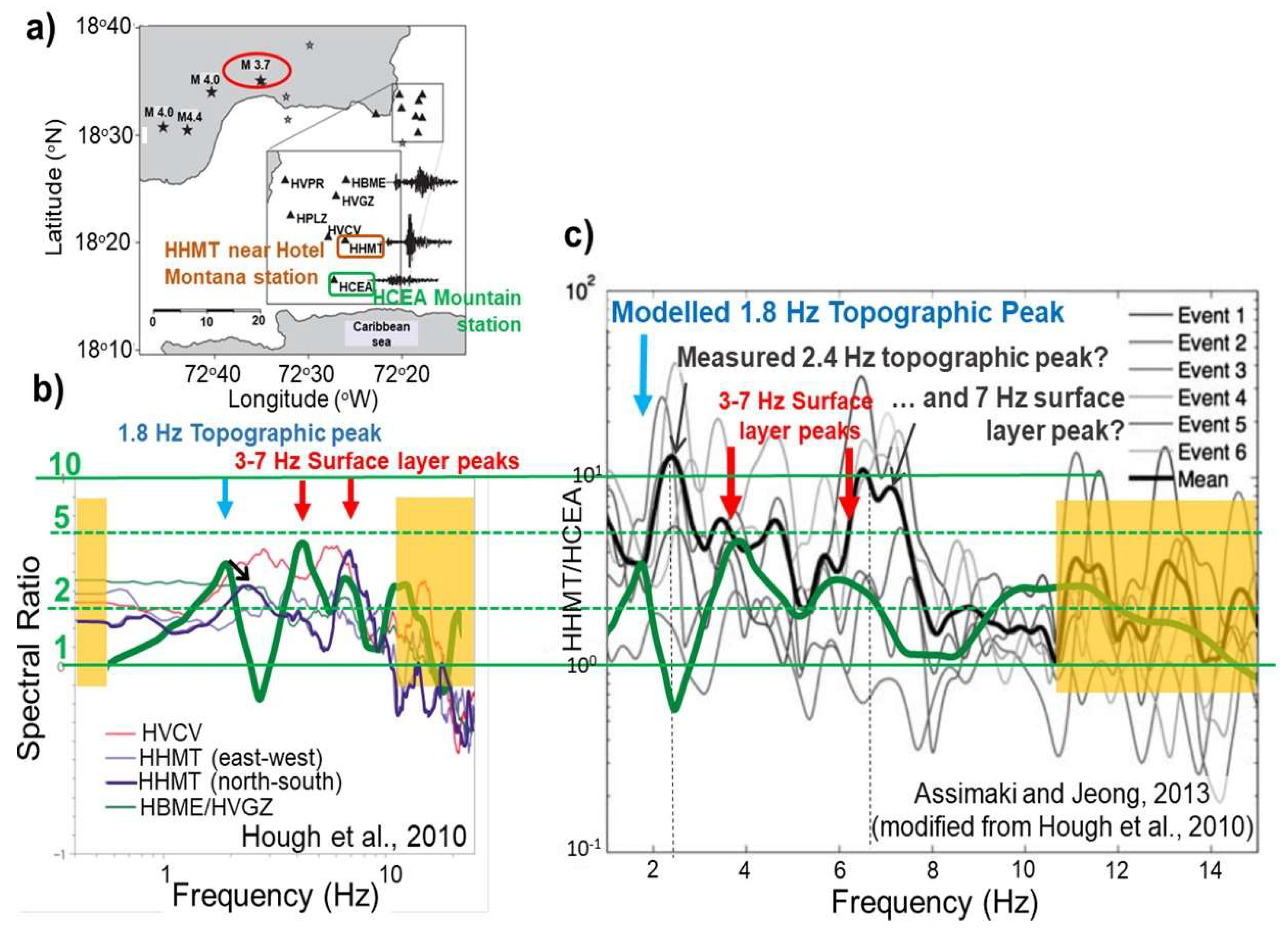
Figure 8b, we included also the SSR graphs for the equivalent HM site computed with respect to the smallest response that had been simulated for a surface receiver, i.e., for S9 that represents the Delmas 60 site (marked by a low altitude and by a thin surface layer), computed respectively for the surface layer model (green curve) and for the purely topographic model (violet curve). By comparing these SSRs with the one computed with respect to the subsurface receiver, it can first be seen that the “topographic” peak is shifted to a higher frequency (from 1.1 to 1.8 Hz) and decreases in amplitude (from 5.2 to, respectively, 3.3 in the surface layer model, and 2.8 in the purely topographic model). Second, the main higher frequency peaks appear in the same frequency range as the SSR peaks computed with respect to the subsurface receiver; they are marked by only slightly smaller amplitudes (reduction from 4.6 to 4.2) in the surface layer model, and by clearly smaller amplitudes (reduction from 4.6 to 2.8 for the larger peak) in the purely topographic model. These observations highlight the importance of the type of reference receiver used for the SSR calculation, and of the fact that, beyond the described changes, the two main amplified frequency ranges stay roughly the same: the lower frequency peaks (near 1–1.8 Hz) are the same for the model with and without surface layer; this confirms that the lower frequency peaks can be attributed to the effect of the topography, while the peaks between 3–7 Hz are significantly smaller in the model without to the surface layer and, thus, are most likely due to the surface layer amplification (which can be combined with topographic effects for some frequencies, as also the SSRs of the purely topographic model shows peaks at those frequencies). Actually, both peaks of the SSR computed for the purely topographic model, the one at1.8 Hz and the other at 3.7 Hz, can be explained by applying the rule of [17], stating that the wavelength amplified by a mountain is of the same order of magnitude as the length of the mountain basis. The entire Gros-Morne hill is composed of a main hill and a small hill, with a length of about 750 m for the basis of this general morphology. Considering a shear wave velocity of 1300 m/s, the amplified frequency is about 1300/750 = 1.6 Hz. The main hill (the NE part) has a basis length of about 370 m, which would induce an amplification at about 1300/370 = 3.5 Hz. Those two frequencies are close to the aforementioned modelled main amplified frequency ranges around 1.8 and 3.7 Hz. Thus, it is likely that the compound hill structure produces two “topographic” amplification peaks, noting that the second one is partly overprinted by surface layer amplification that occurs in the same frequency range. Also the surface layer peaks basically follow the simple 1D layer resonance rule that defines the resonance frequency “f” and the 1D resonance peak amplitude “A”, respectively, by the equations, f = Vs/4h and A = Vs(BR)/Vs(SL), with h being the surface layer (SL) thickness, Vs(SL) being its average shear wave velocity, and Vs(BR) being the one of the bedrock. The expected 1D resonance frequency is about 4.5 Hz (=550/4 × 30), which is close to the 4 Hz of the first and largest surface layer peak. The expected 1D amplification at this frequency would be 2.4 (=1300/550). This amplitude is close to the one of the 4 Hz peak shown by the measured SSRs and NS S-waves HVSR, but lower than the modelled 4 Hz peak amplitude that is larger than 4. Just before, we explained that a possible second topographic amplification occurs near this frequency, which could explain the larger modelled amplification. This discussion about the origin and significance of the measured and modelled ground amplification will be continued in the next section.

4. Discussion

4.1. The Use of HVSR for Site Effect Analysis

Among all geophysical survey results, those of the HVSR have been the most important ones used for constructing the 3D geomodel and for compiling the qualitative site effect maps presented above. The high value and rising popularity of the HVSR for site effect assessment for smaller or larger sites is partly related to the relative “facility” of implementation of the ambient vibration measurements, compared with other geophysical surveys—they can be applied almost everywhere, and due to their rapidity, allow for a much denser network of measurements. Yet, those simple measurements have also clear application limits (see, e.g., [18]). First, the extended use of HVSR is strongly dependent on other geophysical outputs, such as shear wave velocity data, that are needed for thickness calculation. In [3], we discuss the limits related to the direct use of thickness calculation in case of a 2–3D site, on the basis of the simple 1D equation h = Vs/4 f0. The main argument to support this approach in the present case is that the locally computed thickness values are clearly smaller than the observed distances between laterally changing Vs and thickness values; so, we estimate that each measurement site can be considered as a “sub-1D” site. Furthermore, the hill morphology is only pronounced in some places on the southern slope where, anyway, only a few measurements were made. Missing measurements on this slope caused some interpolation problems in the 3D geomodel that had to be solved by inserting additional “artificial” log points, which are not based on measurements.
Second, a very important issue for mapping site effects with HVSR results, in addition to the peak frequencies that can be used for thickness calculation, is related to the interpretation of the HVSR peak amplitudes. For the use of the HVSR amplitude map in terms of site effect indicator, we considered relative amplitude changes, rather than absolute amplitude values. To explain this limited use of HVSR amplitude information, we compare in Figure 9 the 2D modelled SSR (for the surface layer model, using S9 receiver as reference) with the HVSR and with the NS S-waves HVSR that had been measured near Hotel Montana site. First of all, this comparison clearly shows that the all modelled amplitudes are significantly larger than the HVSR peak amplitudes. At low frequency (below 2 Hz), the ambient vibration HVSR does even not present any peaks where the NS S-waves HVSR (from earthquake recordings) and the modelled SSR present clear peaks; thus, the “topographic” peak is missing in the ambient vibration HVSR. A match of peak frequencies is only obtained for the 3–7 Hz frequency range. Thus, we estimate that the low-frequency amplification, likely to be influenced by the general hill topography as explained in the previous section, is not reproduced at all by the ambient vibration HVSR; only some weak resonance effects can be observed for the higher frequency range that was attributed above to surface layer amplification. A similar observation was made by [19], who noted that SSR presents the clearest low-frequency peak for earthquakes recorded along a ridge in the San Francisco Bay area (in their case near 1 Hz). They interpreted this peak as the fundamental one related to topographic amplification. HVSR from earthquake records generally presented a peak, as well, around this frequency, but with a lower amplitude, while they could show that HVSR from short-period ambient noise recordings do not necessarily reproduce the “topographic” peak. Thus, they judged that “ambient noise is found to be a poor source for the study of topographic effects”. With our study, we can confirm this observation, even though there are others (see, e.g., [20]) showing that topographic polarization effects can be analyzed though ambient vibration HVSR, at least if the site presents a clear ridge morphology and simple geological characteristics.
The question remains if topography does not influence, at all, ambient vibrations. Figure 3c above showed that the azimuths of HVSR peaks (above 3 Hz) are clearly changing orientation from one site to another on the Gros-Morne hill, but at almost all sites, preferential shaking is subparallel to the local maximum slope gradient. Thus, even if the general orientation of the hill does not have any direct effect on the peak shaking azimuth (as this would mean that the peak shaking azimuth stays the same all over the hill), the local morphology marked by the slope orientation really seems to influence the peak azimuth. The reason for the stronger shaking along slope dip could be related to slightly weaker elastic properties (notably, marked by lower Vs-values) parallel to the slope gradient, possibly due to relaxation of the surface material in this direction, that may be induced by plastic flow. Interestingly, the NS HVSR computed for S-wave windows of recorded earthquakes present clear low frequency peaks which, in addition, present a NS azimuth subparallel to the short axis of the hill (compare the NS with the EW S-waves HVSR in the graphs a2 and a1 of Figure 2). While ambient vibrations do apparently not help measure topographic effects, at least not those related to a more complex hill or mountain morphology (compared to the site presented by [20] that is marked by a clear ridge and unique lithology with uniform Vs30, Gros-Morne hill has a rough E–W elongation, but cannot be called a clear ridge, and Vs15 values are highly variable over the hill), HVSR applied to S-wave windows of earthquake recordings, do. This might be due to the fact that ambient noise HVSR measures the ellipticity of surface waves, which are not necessarily affected by the global hill morphology (at least not if it is more complex), while the shaking of a mountain induced by an earthquake obviously affects, more intensely, the horizontal component along the short axis than the other horizontal component, and even more than the vertical component.

4.2. Comparison of the Numerical Modelling Outputs with Former SSR Results, Importance of the Reference Station Receiver

In Part A of the Gros-Morne site effect study presented in [3], we presented some comparison of our measured SSR with those that had been published earlier by [5,6]. Below, in Figure 10, we add the modelling results to this comparison, in terms of SSR (green curve) computed with respect to receiver S9, representing the Delmas 60 site. The comparison of the modelled SSR with the SSR measured by [5] in Figure 10b shows that amplification levels are roughly the same; the modelled SSR even presents some slightly larger peaks both in the low and in the higher frequency range.
However, the comparison with the SSRs computed by [6] reveals that the latter are systematically larger (almost by a factor of 2) than our modelled SSR. A common point of these comparisons is the fact that the first SSR peak measured both by [5] and [6], interpreted here as ”topographic” peak, occurs at a slightly larger frequency (at around 2.4 Hz) than the modelled one (observed at 1.8 Hz). A similar frequency shift can be observed for the higher frequency, the assumed “surface layer” peaks. Already in [3], we highlighted the fact that the use of other reference stations can partly explain the differences between the measured SSRs. We used two stations located in the north and in the south of the hill, respectively, while [5,6] used, as reference station, HCEA, that is located on a rock massif at 3 km in the south of Gros-Morne. However, this fact cannot explain why [5,6] the obtained SSRs had different amplitude levels for almost the same dataset. Considering that some differences might be due to the type of recorded event used for SSR computation, we must assume that local ground motion effects near Gros-Morne are also source path- and not only site-dependent. Therefore, in the near future, we plan to develop subregional numerical models to assess the possible effect of guided waves along the main Enriquillo-Plantain Garden Fault and associated smaller faults on ground motions in the southern hilly part of Port-au-Prince.

5. Conclusions

The multiple modelling results presented essentially corroborate the conclusions presented in [3]: thus, we can confirm that the topographic amplification produces the first, near 2 Hz, peak, and possibly also contributes to the next 3.5–4.5 Hz peak, and that surface layer amplification produces site effects starting from 3 Hz. The amplitudes of the modelled peaks, of the SSRs computed by [5], and also of our measured SSRs, indicate that the higher parts of the Gros-Morne hill are affected by moderate to locally medium-strong site effects. However, our results are not in line with the very strong site effects assessed by [6] for the Gros-Morne hill site. Amplification levels of up to a factor of 10 and more, as presented by [6], could not be reproduced by our small 2D model. Yet, we do not exclude that some regional source-path effects might have contributed to the high SSR amplitudes computed by [6].
Anyway, also, the moderate to locally medium-strong sites amplification determined by the present study, measured and modelled over a frequency range between 0.5 and 7 Hz, significantly contribute to local seismic risk, as larger buildings are sensitive to the seismic response in this frequency range. Thus, Hotel Montana was (and the reconstructed building still is) exposed to moderately high site effects. Yet, also without deeper investigations, such moderate to strong local amplification can (and should) always be expected for a hill site such as the one of Gros-Morne. Our studies did not produce any “surprising” results; previous studies on a mountain site in Central Asia such as presented by [21] produced SSR amplitude levels reaching factors of up to 8 over a wide frequency range that were really unexpected for a smooth mountain that is purely made of granitic rocks. Thus, we estimate that the widespread damage observed after the 2010 event in some zones near Gros-Morne hill cannot only be blamed on strong site effects. In particular, our studies showed that the northeastern zone (district of Delmas) is only exposed to weak or medium ground motion amplification and, thus, less damage could be expected for those areas. Therefore, we conclude that widespread damage in that area was mainly due to higher building vulnerability (that has not been assessed in the frame of the present study).

Author Contributions

The research work has been completed by the main author, S.U., who also carried out most of the modelling. Both co-authors D.B. and C.P. helped with the interpretation of the results. The modelling analysis has been supervised by co-author H.-B.H. The manuscript has been prepared in close collaboration between S.U. and H.-B.H., and was corrected by the two other co-authors.

Funding

This work was carried out thanks to the financial support of the Belgian “Académie de Recherche et d’Enseignement Supérieur (ARES)”. It was done in the framework of a PhD thesis that was part of this Belgian-Haitian collaboration project.

Acknowledgments

We thank the team of the Research Unit of Geosciences of the Faculty of Sciences of Haiti State University for their support and collaboration as well as the team of the Technical Unit of Seismology which helped us collect the seismological data. We further thank Phillipe Cerfontaine and Anne-Sophie Mreyen from the Georisk and Environment team of the University of Liege for their assistance.

Conflicts of Interest

The authors declare no conflicts of interest.

References

  1. Frankel, A.; Harmsen, S.; Mueller, C.; Calais, E.; Haase, J. Seismic hazard maps for Haiti. Earthq. Spectra 2011, 27 (Suppl. 1), 23–41. [Google Scholar] [CrossRef]
  2. Symithe, S.; Calais, E. Present-day shortening in Southern Haiti from GPS measurements and implications for seismic hazard. Tectonophysics 2016, 679, 117–124. [Google Scholar] [CrossRef] [Green Version]
  3. Ulysse, S.; Boisson, D.; Prépetit, C.; Havenith, H.B. Site Effect Assessment of the Gros-Morne Hill Area in Port-au-Prince, Haiti, Part A: Geophysical-Seismological Survey Results. Geosciences 2018, 8, 142. [Google Scholar] [CrossRef]
  4. Bilham, R. Lessons from the Haiti earthquake. Nature 2010, 463, 878–879. [Google Scholar] [CrossRef] [PubMed]
  5. Hough, S.E.; Altidor, J.R.; Anglade, D.; Given, D.; Janvier, M.G.; Maharrey, J.Z.; Meremonte, M.; Mildor, B.S.-L.; Prepetit, C.; Yong, A. Localized damage caused by topographic amplification during the 2010 M7.0 Haiti earthquake. Nat. Geosci. 2010, 3, 778–782. [Google Scholar] [CrossRef]
  6. Assimaki, D.; Jeong, S. Ground-motion observations at Hotel Montana during the M 7.0 2010 Haiti earthquake: Topography or soil amplification? Bull. Seismol. Soc. Am. 2013, 103, 2577–2590. [Google Scholar] [CrossRef]
  7. Saint-Fleur, S.; Bertrand, E.; Courboulex, F.; De Lépinay, B.M.; Deschamps, A.; Hough, S.; Cultrera, G.; Boisson, D.; Prépetit, C. Site effects in Port-au-Prince (Haiti) from the analysis of spectral ratio and numerical simulations. Bull. Seismol. Soc. Am. 2016, 106, 1298–1315. [Google Scholar] [CrossRef]
  8. Grelle, G.; Wood, C.; Bonito, L.; Sappa, G.; Reveillino, P.; Rahimi, S.; Guadagno, F.M. A reliable computerized litho-morphometric model for development of 3D maps of Topographic Aggravation Factor (TAF): The cases of East Mountain (Utah, USA) and Port-au-Prince (Haiti). Bull. Earthq. Eng. 2017. [Google Scholar] [CrossRef]
  9. Wathelet, M. GEOPSY Geophysical Signal Database for Noise Array Processing. Software, LGIT, Grenoble. 2005. Available online: www.geopsy.org (accessed on 20 April 2018).
  10. Albarello, D.; Lunedei, E. Combining horizontal ambient vibration components for H/V spectral ratio estimates. Geophys. J. Int. 2013, 194, 936–951. [Google Scholar] [CrossRef] [Green Version]
  11. Fäh, D.; Kind, F.; Giardini, D. A theoretical investigation of average H/V ratios. Geophys. J. Int. 2001, 145, 535–549. [Google Scholar] [CrossRef] [Green Version]
  12. Massa, M.; Barani, S.; Lovati, S. Overview of topographic effects based on experimental observations: Meaning, causes and possible interpretations. Geophys. J. Int. 2014, 197, 1537–1550. [Google Scholar] [CrossRef]
  13. European Commission, International Charter Space and Major Disasters, SERTIT Haiti Port-au-Prince Building Damage, Assessment per Urban Block. Available online: http://sertit.u-strasbg.fr/applications.html (accessed on 22 April 2018).
  14. Cox, B.R.; Bachhuber, J.; Rathje, E.; Wood, C.M.; Dulberg, R.; Kottke, A.; Olson, S.M. Shear wave velocity-and geology-based seismic microzonation of Port-au-Prince, Haiti. Earthq. Spectra 2011, 27, 67–92. [Google Scholar] [CrossRef]
  15. Cundall, P.A. A Computer Model for Simulating Progressive, Large-Scale Movements in Blocky Rock Systems; Rock Mechanics: Nancy, France, 1971. [Google Scholar]
  16. Bathe, K.-J.; Wilson, E.L. Numerical Methods in Finite Element Analysis; Prentice-Hall: Upper Saddle River, NJ, USA, 1976. [Google Scholar]
  17. Geli, L.; Bard, P.Y.; Jullien, B. The effect of topography on earthquake ground motion: A review and new results. Bull. Seismol. Soc. Am. 1988, 78, 42–63. [Google Scholar]
  18. Lachet, C.; Bard, P.Y. Numerical and Theoretical Investigations on the Possibilities and Limitations of Nakamura’s Technique. J. Phys. Earth 1994, 42, 377–397. [Google Scholar] [CrossRef]
  19. Hartzell, S.; Meremonte, M.; Ramírez-Guzmán, L.; McNamara, D. Ground Motion in the Presence of Complex Topography: Earthquake and Ambient Noise Sources. Bull. Seismol. Soc. Am. 2014, 104, 451–466. [Google Scholar] [CrossRef]
  20. Panzera, F.; Lombardo, G.; Rigano, R. Evidence of Topographic Effects through the Analysis of Ambient Noise Measurements. Seismol. Res. Lett. 2011, 82, 413–419. [Google Scholar] [CrossRef]
  21. Havenith, H.B.; Jongmans, D.; Faccioli, E.; Abdrakhmatov, K.; Bard, P.-Y. Site effects analysis around the seismically induced Ananevo rockslide, Kyrgyzstan. Bull. Seismol. Soc. Am. 2002, 92, 3190–3209. [Google Scholar] [CrossRef]
Figure 1. (a) Distribution of the horizontal to vertical spectral ratio (HVSR) results on the geological map (see on the right the location on larger general geological map); the size of the circle indicates the amplitude level. The circle color represents the f0 values. (b) Distribution map of shear wave velocity over the first 15 m of depth with locations of the seismic stations at Hotel Montana (HM), Delmas 60, and at FIC.
Geosciences 08 00233 g001
Figure 2. Comparison between the standard spectral ratio (SSR) and S-wave HVSR results for station Hotel Montana (HM). (a) SSR computed with respect to FIC station, in (a1) for the E–W component, in (a2) for the N–S component; (b) SSR computed using the Delmas 60 station as reference, in (b1) for the E–W component, in (b2) for the N–S component. In both subfigures (a,b), the black curve represents the S-wave HVSR for HM station, and the green dashed curve shows the average SSR for HM computed with respect to the averaged FIC-Delmas 60 spectra (combination of two reference stations); see also dashed curve of E–W S-waves HVSR in (a1,b1) and grey curve of N–S S-waves HVSR in (a2,b2).
Geosciences 08 00233 g002
Figure 3. Maps showing the distribution of HVSR characteristics (see also the location of the seismic stations). Map (a) presents the interpolated values of the resonance frequency of the main peak; map (b) outlines the distribution of the HVSR amplitude values; map (c) shows the polarization of the HVSR shaking at the main peak for each measurement (see red double-arrows indicating strongest shaking direction) and for a group of measurements (black double arrows).
Geosciences 08 00233 g003
Figure 4. Map (a) outlines the distribution of the combined HVSR resonance frequency and peak amplitude site effect characteristics; map (b) presents the interpolated Vs15-values; map (c) presents the distribution of the damages; the red line delimits the study area; modified from [13].
Geosciences 08 00233 g004
Figure 5. 3D Geomodel of the Gros-Morne site combining HVSR and multichannel analysis of surface waves (MASW) results. The three layers correspond to the assumed bedrock (green), to the soft rock on top of the bedrock (yellow layer with basis obtained through interpolation of the bottom of the log-bars); in some parts, a near-surface layer (brown) was added on top of the soft rock. (a) Initial model realized only with the recorded data, but presenting interpolation problems. (b) Layer-view of corrected model with HVSR log-bars with the contact surfaces corresponding to the interpolation of the layer contacts within the logs. (c) Volume-view of corrected model with recorded and added HVSR (blue balls = data; red balls = added); the white balls are seismic stations. (d) Same as (c), but along an E–W section. (e) Map-view of the geomodel. See red ellipse in some subfigures, marking the extrapolation problem that appears mainly outside the target area (highlighted by a white rectangle).
Geosciences 08 00233 g005
Figure 6. Map (a) outlines the distribution of the combined HVSR resonance frequency and peak amplitude site effect characteristics. (b) Map-view of the geomodel with stars marking the station locations and triangles the location of surface receivers in the numerical model presented in 3.3. (c) Section used for numerical modelling, including a simplified single layer (see indication of approximate 30 m thickness on top of the hill)—on top of bedrock structure, with main elastic properties described in the table to the left. Sx indicates the surface receiver locations; a reference receiver was included inside the bedrock.
Geosciences 08 00233 g006
Figure 7. Processing of the modelled site response in terms of standard spectral ratio (SSR in the left graph, in black, together with S14 spectrum in light grey and reference receiver spectrum multiplied by two in dark grey) exemplified for the S14 receiver that corresponds to the equivalent Hotel Montana (HM) site along the 2D section (near the hill top). As reference receiver, a subsurface receiver was used, whose response was multiplied by a factor of two (see dashed signal in lower right part of the figure, as well as the doubled spectrum amplitudes in grey) to represent the one of a rock surface receiver in the same model. See also parts of spectrum with low energy content (not used for analysis) marked by orange semi-transparent mask.
Geosciences 08 00233 g007
Figure 8. (a) SSR graphs for several surface receivers distributed along the 2D numerical section. For the equivalent HM site, the modelled SSR is compared with the measured NS SSR obtained with respect to the FIC (in blue) and with the Delmas 60 station (in red). The first and second amplification peaks are marked, respectively, by a blue and by two red arrows. (b) The modelled equivalent HM SSR (black curve) is compared with the measured NS S-waves HVSR of HM site (grey curve) and the SSR result (beige) from a purely topographic model (surface layer with identical properties as bedrock). The green and violet curves represent the SSRs of the equivalent HM site with respect to surface Reference 2 receiver S9 = Delmas 60, in the surface layer model (marked in green), and the purely topographic model (marked in violet), respectively. See blue arrow marking the shift of the first peak and the red arrows indicating the second layer peaks. See also parts of spectrum with low energy content in the input signal (not used for analysis) marked by an orange semi-transparent mask.
Geosciences 08 00233 g008
Figure 9. Simulated surface layer model SSR for the equivalent HM site computed with respect to S9 receiver (representing the Delmas 60 site, see green curve) compared with measured NS S-waves HVSR (grey curve) and the noise HVSR presented by [3].
Geosciences 08 00233 g009
Figure 10. (a) Map of stations and recorded aftershocks (from [6]) with highlighted Hotel Montana and HCEA bedrock station (on hard limestone) in the mountain massif to the south of Gros-Morne hill. (b) Simulated surface layer model SSR for the equivalent HM site computed with respect to S9 receiver (representing the Delmas 60 site, see bolt green curve) compared with the spectral ratios for several sites inside and near Port-au-Prince, presented by [5], on the basis of recorded aftershocks of the 12 January 2010, event (the N–S spectral ratio for Hotel Montana, HHMT, computed with respect to mountain station HCEA, is shown by the highlighted violet curve); the same modelled SSR (bolt green curve, with changed amplitude and frequency scale) is compared in (c), with the spectral ratios obtained for the 2010 aftershock dataset analyzed by [6] for Hotel Montana. Several amplification levels are marked by green lines. See also parts of spectrum with low energy content in the modelled input signal marked by an orange semi-transparent mask.
Geosciences 08 00233 g010

