Article

One-Dimensional Nonlinear Seismic Response Analysis Using Strength-Controlled Constitutive Models: The Case of the Leaning Tower of Pisa’s Subsoil

1
Department of Architecture, Roma Tre University, 00153 Rome, Italy
2
College of Civil Engineering, Fuzhou University, Fuzhou 350108, China
3
Department of Civil and Industrial Engineering, University of Pisa, 56122 Pisa, Italy
*
Author to whom correspondence should be addressed.
Geosciences 2018, 8(7), 228; https://doi.org/10.3390/geosciences8070228
Submission received: 18 April 2018 / Revised: 11 June 2018 / Accepted: 19 June 2018 / Published: 22 June 2018

Abstract

:
The Leaning Tower of Pisa was built between 1173 and 1360 and began to lean at the beginning of its construction. Extensive investigations to reveal the causes of the tilting only began in the early 20th century. Although few earthquakes have been recorded, there is a renewed interest in the seismic behavior of the tower triggered by the availability of new data and technologies. This paper highlights the influence of using new strength-controlled constitutive models in case of 1D nonlinear response analysis. This is an aspect that has been poorly investigated. Most of the computer codes currently available for nonlinear seismic response analysis (SRA) of soil use constitutive models able to capture small-strain behavior, but the large-strain shear strength is left uncontrolled. This can significantly affect the assessment of a 1-D response analysis and the Leaning Tower’s subsoil can be useful for this study as it represents a well-documented and well-characterized site. After a geological and geotechnical description of the subsoil profile and a synthesis of available data, the seismic input is defined. One-dimensional SRAs were carried out by means of a computer code which considers an equivalent-linear soil modelling and two codes which assume nonlinear soil response and permit to use strength-controlled constitutive models. All the parameters were calibrated on the basis of the same soil data, therefore allowing for a direct comparison of the results.

1. Introduction

The Leaning Tower of Pisa was built between 1173 and 1360, and many attempts were made during the construction to correct the undesired tilt. The tower is in the form of a hollow cylinder surrounded by six loggias with columns and vaults merging from the base cylinder and surmounted by a belfry. The structure is subdivided into eight levels called ‘orders’. The outer surfaces are made with marble, while the inner ones with various masonry materials. The annulus between the outer and inner surfaces is filled with rubble and mortar. A spiral staircase winds up within the annulus up to the 6th order, while two shorter spiral staircases lead to the floor and top of the belfry. The staircase forms a large opening on the south side just above the level of the first cornice, where the thickness of the masonry suddenly decreases. The high stress within this region was a major cause of concern since it could give rise to an abrupt brittle failure of the masonry.
Extensive instrumental measurements and investigations started only in the 20th century, as illustrated in [1]. The plane of maximum inclination is approximately coincident with the north-south plane. From 1993 to 2001 the Committee for the Safeguard of Leaning Tower of Pisa carried out several interventions aimed at geotechnical stabilization [2] and structural strengthening [3].
A comprehensive description of the history of the construction of the Tower and interventions is described in [2]. A dynamic monitoring system was installed by the Committee for the Safeguard of the Leaning Tower of Pisa at the end of its activities in 2001. During the last 20 years, several low-intensity earthquakes have been recorded. Although few events and very slight damage related to earthquakes has been observed from the construction of the monument, there is a considerable interest in the seismic behavior of the tower [4,5,6,7] triggered by the availability of new data and technologies. Within the chain starting from seismogenic zones and up to the tower, the dynamic response of its subsoil holds a crucial importance, particularly in terms of the frequency content of seismic input. This paper presents some results showing the influence of using new strength-controlled constitutive models in case of 1D nonlinear response analysis. This is an aspect poorly investigated up to now. Most of the codes currently available for nonlinear seismic response analysis use constitutive models able to capture small-strain behavior, but the large-strain shear strength is not controlled. The development of hyperbolic models (for example the Modified Kondner–Zelasko [8]), in the last decades permitted to well capture the backbone stress–strain curve and the unloading-reloading response of the soil. These models are fit to the experimental or reference shear modulus reduction curves and damping ratio curves but are unable to give realistic results in case of medium-large strain levels, resulting in soil layers strength underestimation or overestimation. This fact can significantly affect the assessment of a 1D site response analysis.

2. Subsoil

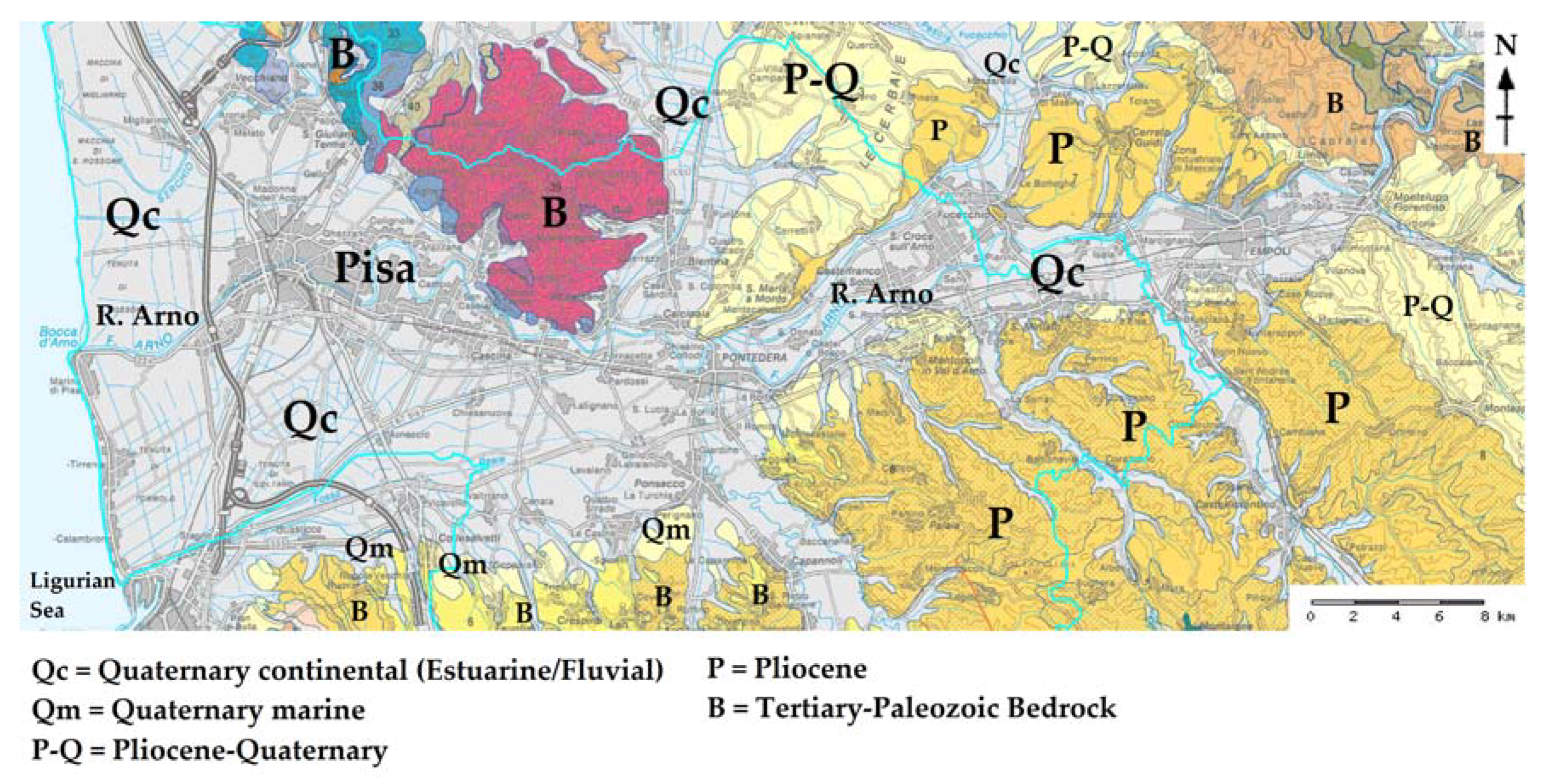
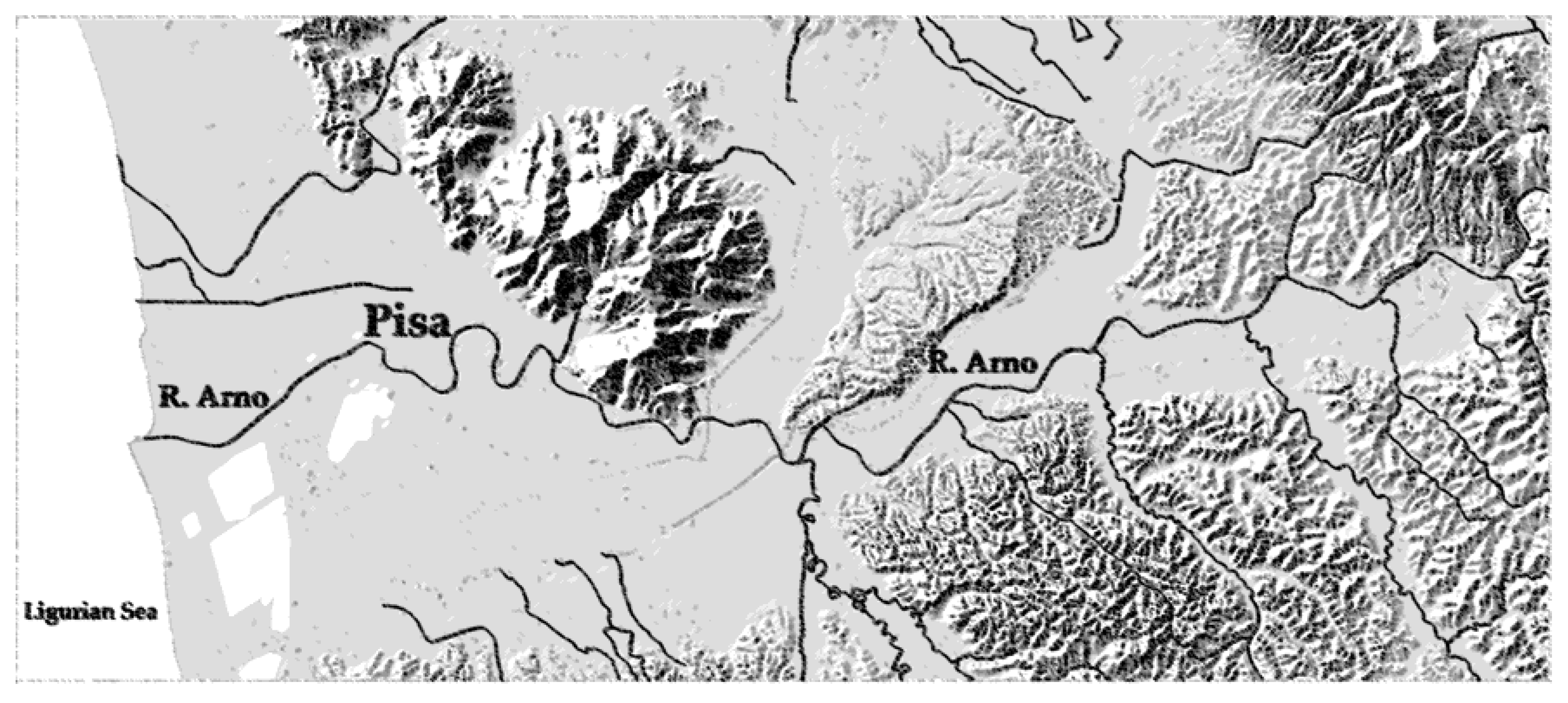
2.1. Geological Description of the Study Area

The current configuration of the Pisa plain comes from the dynamic interaction between erosive and depositional processes developed, starting from the end of the Last Glacial Maximum expansion, first in coastal and transitional marine environments. Then, in the Middle Ages, it evolved mainly in continental fluvial-lake environments.
The proximity to the coast provided the environmental conditions, since prehistoric times, to the development of the anthropic settlement in the area on which Pisa will rise and in the entire coastal area. Figure 1 shows a geological map of the valley of the Arno river, from Florence to the Tyrrhenian (Ligurian) Sea. The mountains positioned to the east of Pisa consists of formations belonging to the Paleozoic and the Tertiary geological periods and their structures reveal intense tectonic deformations.
The main structure is oriented towards NNW-SSE, with faults bordering the western part of the mountains and located 5 km northeast of Pisa.
More recent deposits, identified as quaternary continental in the geological map, developed in marine and in fluvial-lacustrine environments and deposited mainly in an estuary environment.
The valley of the Arno river crosses a mountainous territory starting from its source, in the Tuscan–Emilian Apennines, up to Florence (Figure 1). During the Last Glacial Maximum, in the period between 23,000 and 15,000 years ago, the level of the sea lowered at least 100 m and the river dug a deep valley west of Florence. This valley is now filled with alluvial materials.
Pisa rises on these alluvial deposits, at an elevation of 3–4 m above the present mean sea level. The thickness of alluvial sediments near the city is at least 300 m. In the Piazza dei Miracoli area, at the depth of about 40 m below the ground surface level can be found marine sands deposited during the Flandrian transgression.
Above these dense sands layers, partly rearranged due to wind action, a complex mainly composed by clayey soils can be found. The clay layer close to the surface level is a clayey marine deposit, which was formed in a period of rapid eustatic lifting of the sea level. Figure 2 shows the morphological map of the valley of the Arno river.

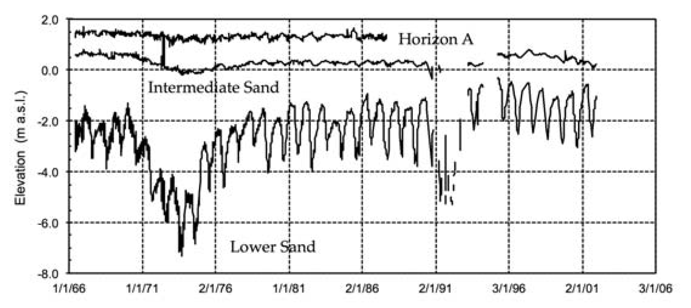
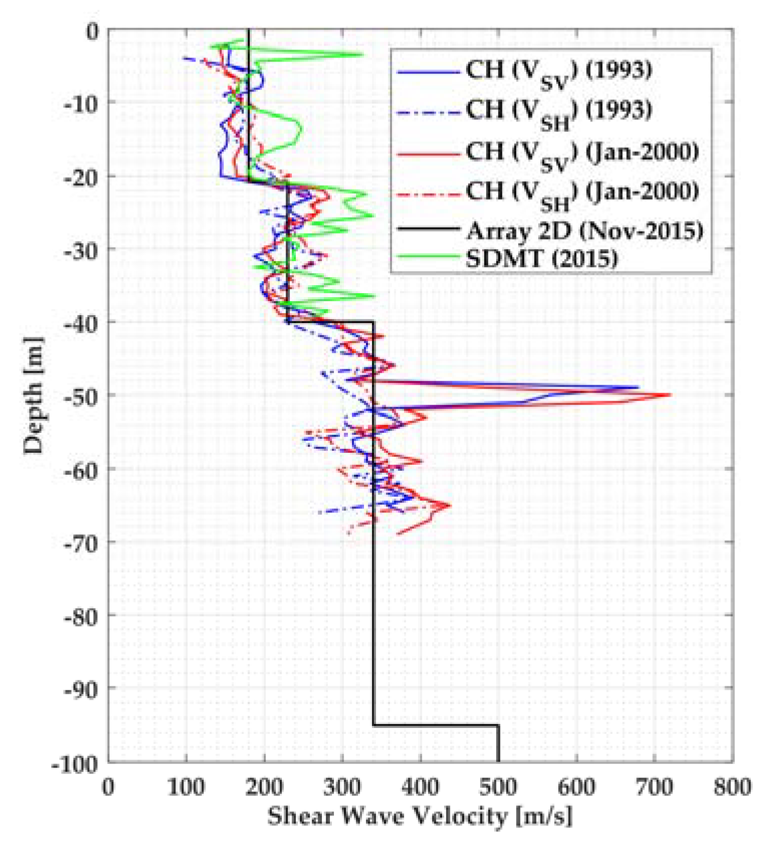
2.2. Geotechnical Model of the Leaning Tower of Pisa Subsoil
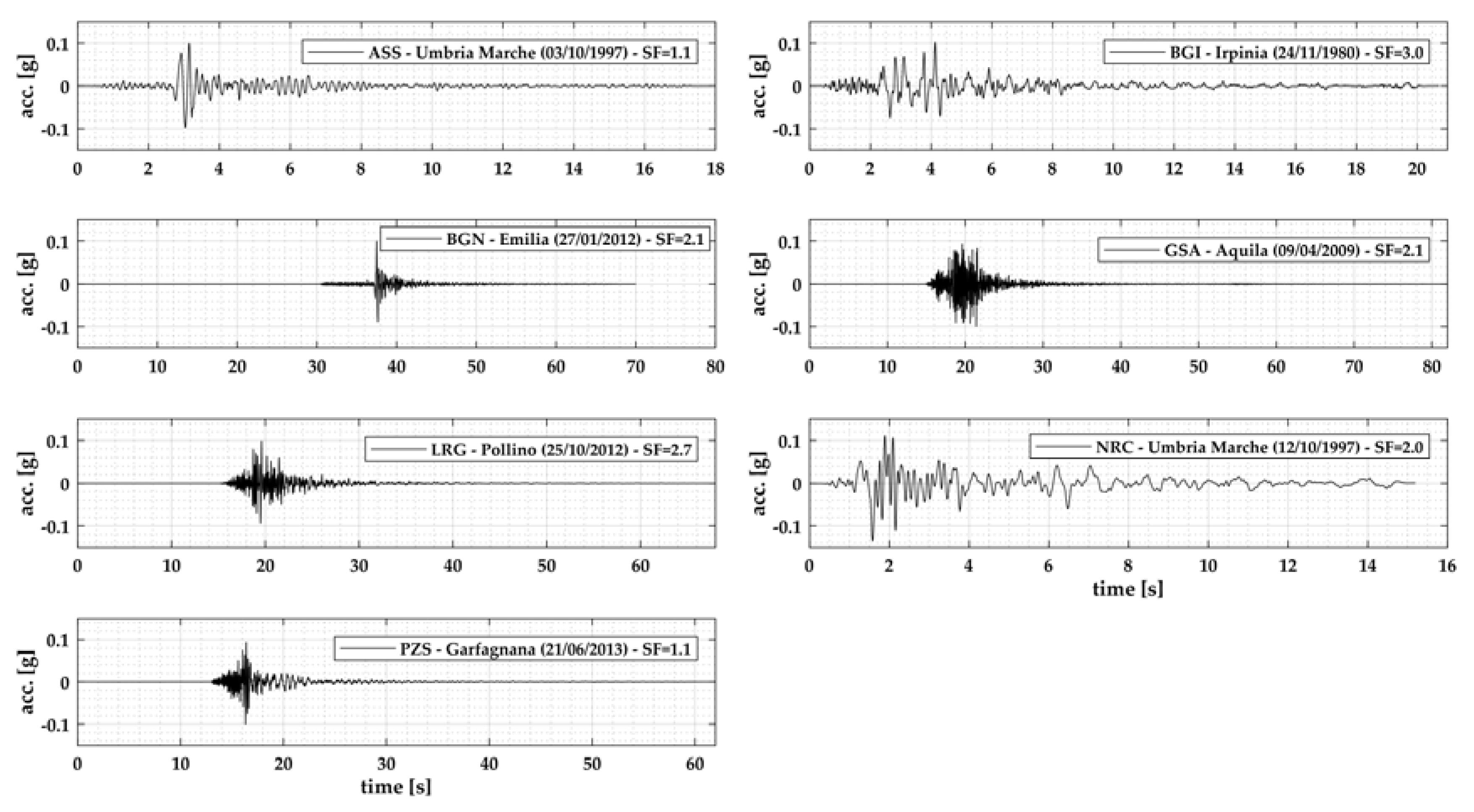
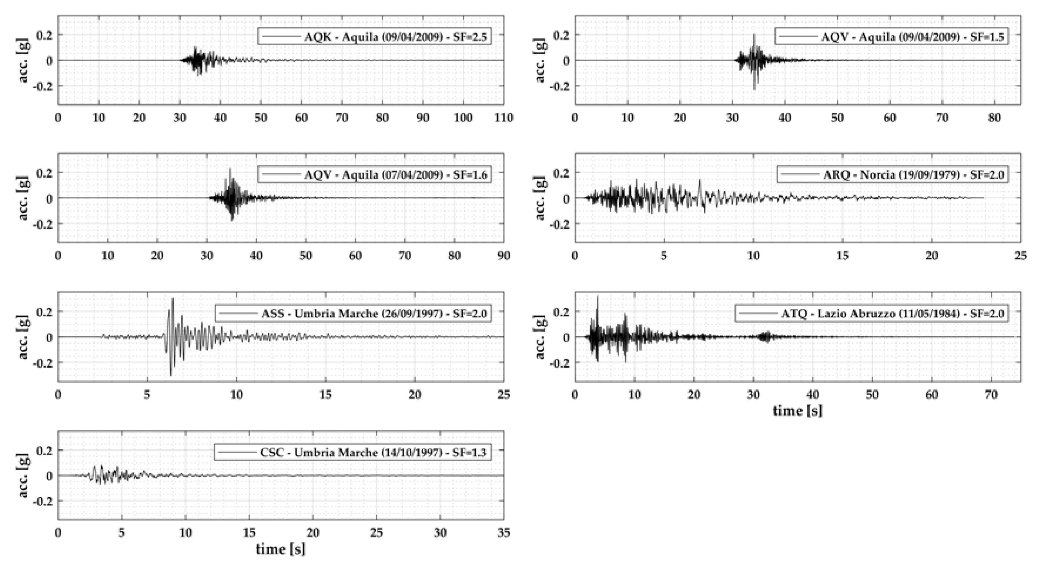
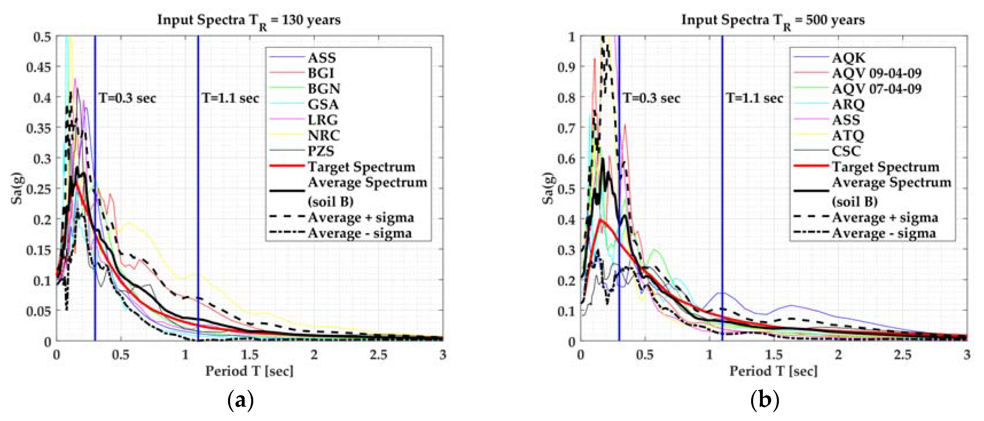
The soil profile under the tower is shown in Figure 3. It consists of three distinct horizons. Horizon A is about 10-m thick and primarily consists of estuarine deposits, laid down under tidal conditions with a rather erratic sequence of sandy and clayey silt layers. Typically of estuarine deposits, there are significant variations over short horizontal distances. At the bottom of horizon A there is a 2-m thick medium dense fine sand layer (i.e., upper sand). Horizon B consists primarily of marine clay, which extends down to a depth of about 40 m. It is subdivided into four distinct layers. The upper layer is soft sensitive clay, locally known as Pancone. It is underlain by an intermediate layer of stiffer clay, which in turn overlies a sand layer (the intermediate sand). The bottom layer of horizon B is a normally consolidated clay known as the lower clay. Horizon B is very uniform laterally near the tower.
Horizon C is composed of dense sand (the lower sand), which extends down to a considerable depth. Based on sample descriptions and piezocone tests, the materials to the south of the tower appear to be more silty and clayey than to the north, and the upper sand layer is locally thinner. This is believed to be the cause of the southward tilt of the tower [11].
The water table in horizon A is found at a depth between 1 and 2 m below the ground surface; the latter has an average elevation of 3 m above mean sea level. Pumping from the lower sand has resulted in downward seepage from horizon A with a pore pressure distribution with depth which is slightly below hydrostatic (Figure 4).
Many borings beneath and around the tower show that the surface of the Pancone clay stretches out beneath the tower, from which it can be deduced that the average settlement of the monument is more than 3 m (Figure 3).
A comprehensive description of subsoil investigations carried out since the beginning of the 20th century can be found in [11], whereas the dynamic characterization of subsoil is the focus of the present paper.
As reported in [12], several tests were performed from the early 1990s to determine the shear wave velocity profile Vs, namely Down Hole (DH) test [13], Cross Hole (CH) test, DH and CH tests [11] and an SDMT test (Seismic Dilatometer Test). The results obtained from these tests show a satisfactory agreement of the Vs values. All the tests reached a maximum depth of 40 m except for the CH test, which reached a depth of 65 m. None of the tests was successful in identifying the seismic bedrock.
The bedrock (i.e., Vs ≥ 800 m/s) is presumed to be very deep and some attempts have been made to increase the knowledge of the subsoil below 65 m depth. An array 2D test has been exploited to obtain the shear wave velocity profile down to more than one hundred meters from ground surface [6]. Figure 5 shows the shear velocity profile down to a depth of 100 m. The array 2D test revealed the presence of a stiffer layer (i.e., Vs ≈ 500 m/s) at a depth of about 100 m. Another methodology to investigate about the seismic bedrock depth by using the available H/V ratios is described in [14,15], however further studies and investigations have been planned in order to improve the knowledge of subsoil below 100 m depth.
Many samples have been retrieved from the ground around the tower. Several of these samples have been subjected to laboratory tests to obtain the dynamic characterization of the subsoil. Further information can be found in [11].

3. Seismic Input

Defining the seismic input is a key step in forecasting the seismic action on a structure. Especially when the bedrock depth is defined, the assessment of the seismic hazard is usually based on well-established studies [16].
Ancient monumental masonry buildings are particularly vulnerable to vibrations and specifically to seismic actions due to many factors: in the case of the Tower of Pisa, the construction process lasted two centuries, its characteristic inclination and the several changes in the foundation system occurred during its life contributed to increase the uncertainty in the dynamic behavior. Therefore, it is necessary to define the seismic input in terms of natural accelerograms, which can be scaled in order to match a target response spectrum. In this context, the use of the design response spectrum defined by the Code (e.g., EC8) is not recommended [17], as it has no direct relationship with a specific earthquake characterized by magnitude M and source-to-site distance R, necessary to select sets of natural accelerograms. To this aim, it is appropriate, as reported in recent studies applied to archeological sites [18] to use a hybrid approach which can be briefly summarized as follows:
  • Definition of a Uniform Hazard Spectrum (UHS) obtained by means of a Probabilistic Seismic Hazard Assessment [19] using one or more Ground Motion Predictive Equation (GMPE);
  • Disaggregation of the seismic hazard to obtain the most likely combinations of M and R for a given return period (RP) [20];
  • Definition of a Scenario Earthquake selected from the seismic catalogue, compatible with the previously defined UHS, and evaluated with the same GMPEs of point 1.
On the basis of past studies [6], the target response spectrum was defined for two return periods (RPs) of the seismic action, namely RP = 130 years (moderate earthquake) and RP = 500 years (severe earthquake). First, the disaggregation of the seismic hazard was performed, thus providing a scenario earthquake for each return period. Based on the Italian seismic catalogue CPTI15 [21], two controlling earthquakes were identified [12]: a MW 5.15 seismic event with R (epicentral distance) = 19 km was selected for an RP of 130 years (Livorno 1742) whereas a MW 5.71 earthquake with R = 21 km (Orciano Pisano 1846) was considered for an RP of 500 years.
The GMPE proposed by Akkar and Bommer [22] was then used to evaluate the target response spectra for a Ground Type B (according to the Eurocode 8 [23] and the Italian Building Code NTC-08 [24]), including the subsoil term of the equation depending on the Vs,30 value of the site, which is an average shear wave velocity of the first 30 m. Seven accelerograms were selected for each return period from the European Strong Motion Database [25], considering 5 < M < 5.5 for RP = 130 years and 5.3 < M < 6.2 for RP = 500 years. The horizontal components of the selected accelerograms were scaled so that a good match was obtained between the average spectrum of the seven accelerograms of each set and the reference target spectrum in the range of natural periods 0.31–1 s. This was done to take into account the natural periods of the first two bending modes of the tower and that of the third mode (about 0.3 s), thus obtaining a scale factor (SF) for each record. Figure 6 and Figure 7 depict the time histories of the scaled accelerograms for an RP of 130 and 500 years, respectively, as well as the scale factor used to obtain the final accelerograms.
Figure 8 reports the selected input motion spectra and the results in terms of average response spectrum for 130 years (left) and 500 years (right). The dispersion of the records (average spectrum (μ) ± 1 standard deviation (σ)) is reported for the two cases. For RP = 130 years, the dispersion is large, with a maximum COV (σ/μ) of 0.996 in the range 0.31–1 s, while for RP = 500 years there is a large dispersion too, but slightly lower compared to RP = 130 years, and a maximum COV of 0.643 in the above cited range.

4. Site Response Analysis

The subsoil model adopted for site response analyses is reported in Table 1. The thickness and unit weight for each lithotype were assumed on the basis of the data reported in [11]. The assumed shear wave velocity profile is also based on the outcomes of the 2D seismic array test [6]. However, this profile satisfactorily matches the Vs values measured by other geophysical tests in the upper part. According to the Vs profile, the seismic bedrock (Vs > 800 m/s) is not localized in the explored depth range because a Vs equal to 500 m/s is reached in the lower strata. For this reason, considering the uncertainties in the location of the seismic bedrock (Vs > 800 m/s), the accelerograms selected for the site response analysis were recorded at Ground Type B, according to Eurocode 8 definition. Regarding the nonlinear properties, most of lithotypes were characterized with resonant column (RC) tests.
The A1 lithotype, was characterized within this study through a recently performed resonant column (RC) test. The corresponding results are reported in Figure 9 in terms of normalized secant shear modulus (Figure 9a) and damping ratio (Figure 9b) variation as a function of the shear strain amplitude (G/G0 and D-γ curves).
Because of the lack of experimental data, G/G0 and D-γ curves that have been reported in the literature for similar soils were employed for the remaining lithotypes: MG, A2, B6, C1, C2 and C3 [26,27] (Table 1).
These literature curves have been obtained by a huge database of samples and can quantitatively capture the dynamic behavior of the above lithotypes because are based on the grain size distribution, the plasticity index and the soil stress state. Considering the unavailability of the experimental curves, those proposed by Rollins [26] and by Darendeli [27] are a good compromise for the dynamic characterization of the MG and A2, B6, C1, C2, C3, respectively.
In order to compare the results obtained with different 1-D SRA models, analyses were carried out by means of three different computer codes: equivalent-linear code STRATA [28], nonlinear code DEEPSOIL [29,30,31] and nonlinear code ONDA [32,33]. All parameters for the calibration of the models were deduced from the same group of in situ and laboratory tests.
The analyses were carried out considering a one-dimensional geometry. This choice is justified by the fact that all the main layers are horizontally stratified, and it can be reasonable to assume a geotechnical subsoil model indefinitely extended horizontally.
The seismic wave field was simplified with SH-waves vertically propagating from the bedrock to the soil deposit surface. The input motion was considered as an outcrop motion and was deconvoluted by the computer codes used in this work down to the depth of the base layer.

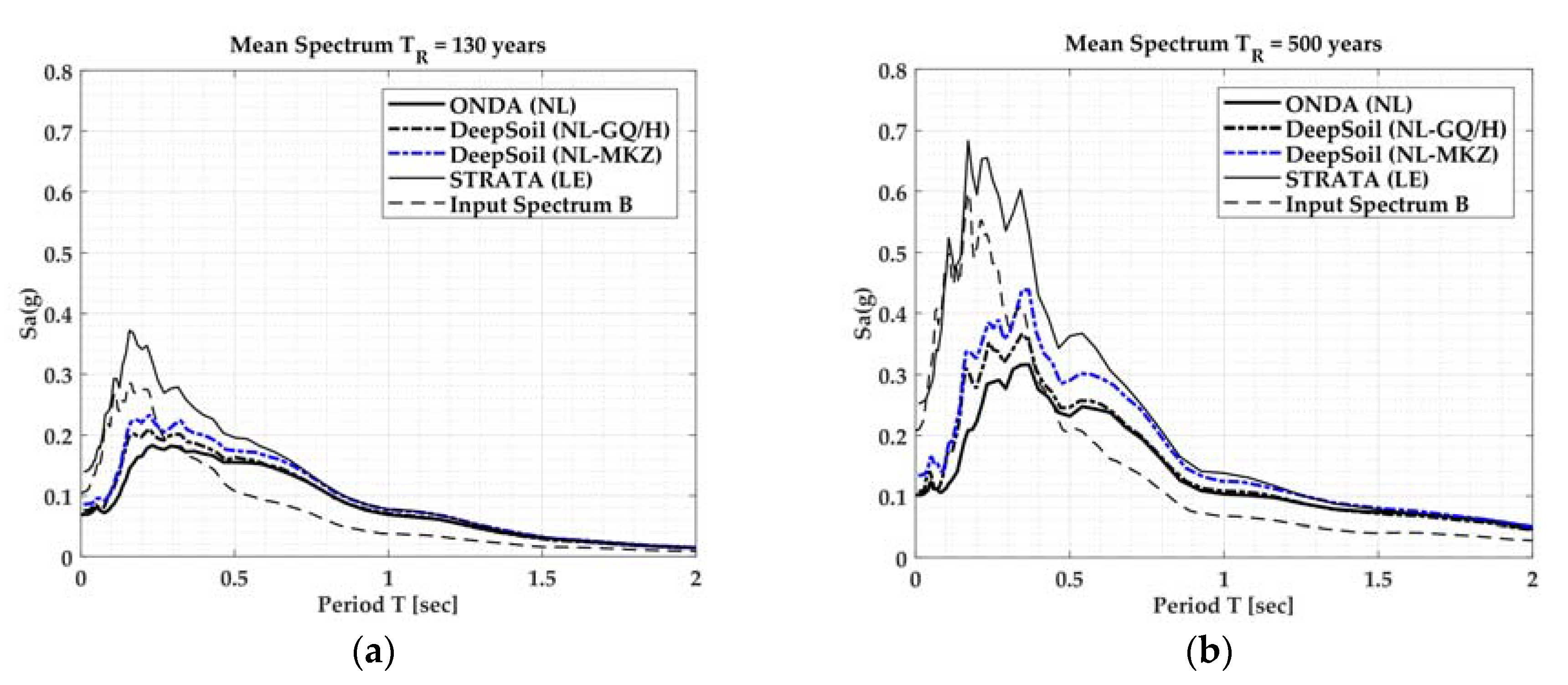
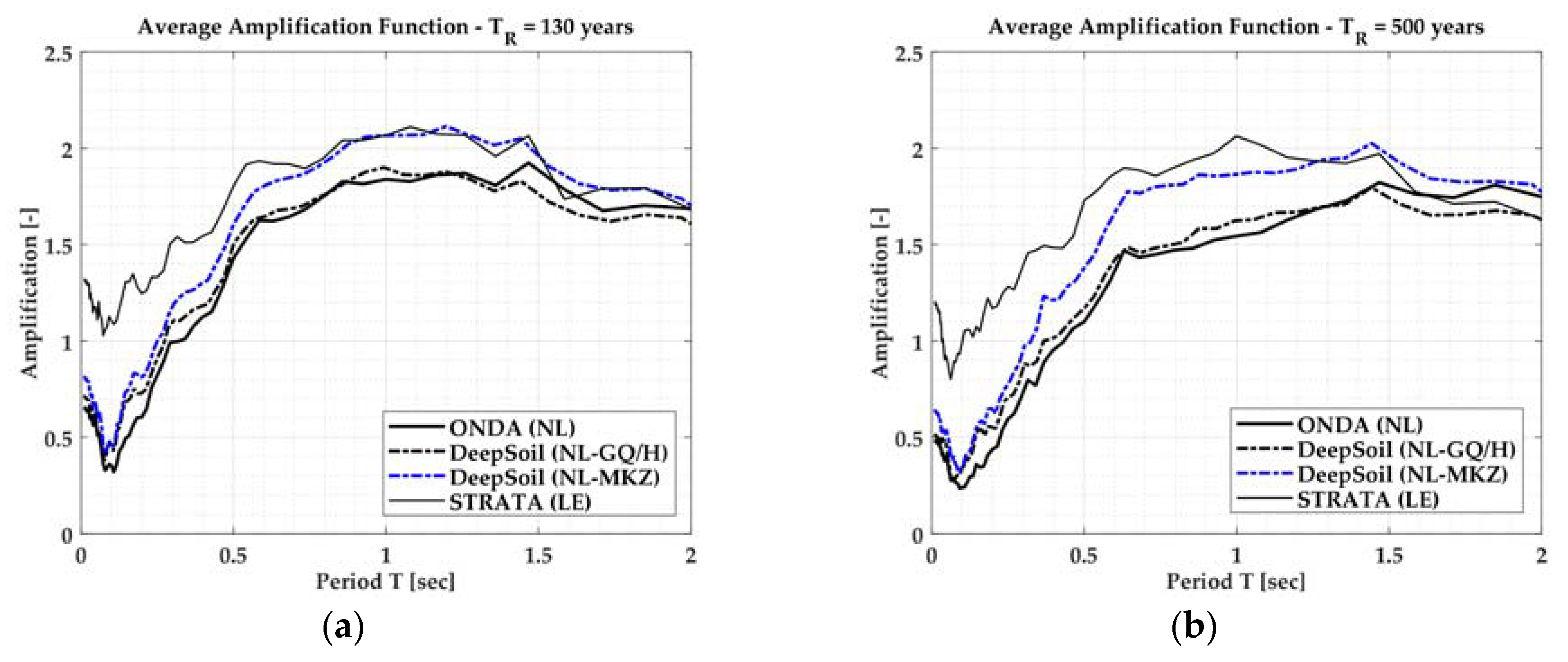
4.1. Seismic Response Analyses with Equivalent-Linear Models

The equivalent-linear (EL) analyses with STRATA were carried out in the frequency domain, and the amplification function was computed. The variation of the shear moduli and of the damping ratios were dependent only on the shear strain level. This means that the material damping has only a frequency independent component. The effective shear strain eff) for a given soil layer and for a given stress time history was evaluated following the suggestions in [34] (Equations (1) and (2)).
γ e f f = R γ max
R = M 1 10
where R is the effective strain ratio, γmax is the maximum shear strain computed in a layer and M is the magnitude related with the acceleration time history considered. This quantity is representative of the time history duration (i.e., number of cycles).
The effective shear strain is needed in order to identify, by an iterative procedure based on G-γ and D-γ curves of each stratum, a strain level which is representative of a given stress time history and therefore to select appropriate values of the shear modulus G and damping ratio D.

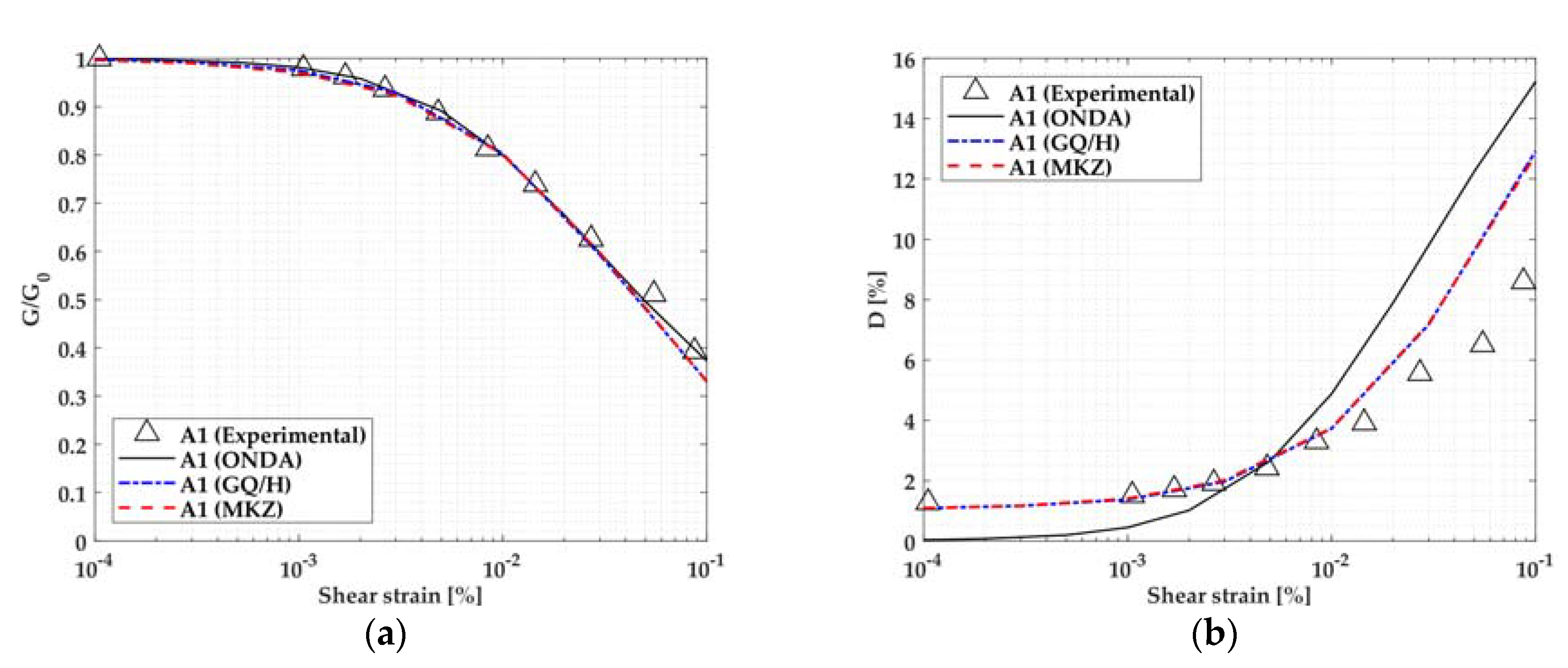
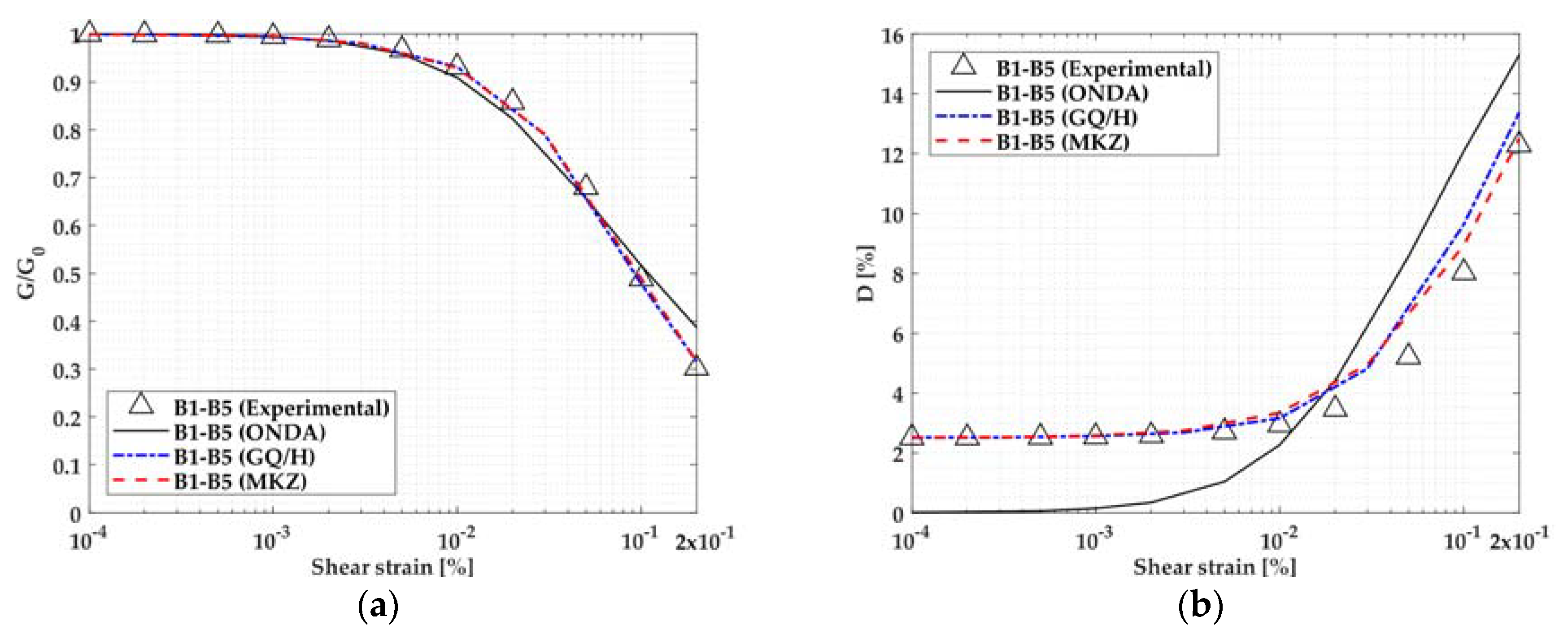
4.2. Seismic Response Analyses with Nonlinear Models

Nonlinear analyses with ONDA and DEEPSOIL are performed in the time domain with a step-by-step integration of the equations of motion of a multi-degree of freedom lumped parameters model. For that purpose, in ONDA [32] the Wilson-θ time integration method was adopted [35], whereas in DEEPSOIL [29] the dynamic equilibrium equation is solved numerically at each time step using the Newmark-β method [36].
In ONDA, the constitutive law (τ-γ) of the initial loading stress–strain curve (backbone or skeleton curve) is represented by the Ramberg–Osgood model [37]. This model consists of a not invertible relationship that depends on four parameters: α and R represent the position and the curvature of the skeleton curve, respectively, while τmax and G0 represent the soil shear strength and the shear modulus at small strain levels, respectively. ONDA uses a strength-controlled constitutive model. The backbone curve can be written in this form:
x = y ( 1 + α | y | R 1 )
where x and y are the normalized shear strain and shear stress, respectively:
x = γ γ r e f
γ r e f = τ max G 0
y = τ τ max
α and R were obtained by a linear interpolation of data collected from Resonant Column tests [11] for lithotypes A1, B1, B2, B3, B4, B5, B7, B8, B9 and B10, while for lithotypes MG, A2, B6, C1, C2 and C3 by a linear interpolation of data based on the modulus reduction curves reported in Table 1. For that purpose, the Ramberg–Osgood equation was rewritten as follows:
log ( G 0 G 1 ) = ( R 1 ) log ( τ τ max ) + log ( α )
Considering Equation (7) and performing a linear regression of the experimental and literature curves data, α and R were obtained.
In Equation (7), the soil shear strength (τmax) was computed according to Equation (8), as proposed by Hardin and Drnevich [38], nevertheless other relationships can be used.
τ max = { [ ( 1 + K 0 ) 2 σ ' v 0 s e n φ + c ' cos φ ] 2 [ ( 1 K 0 ) 2 σ ' v 0 ] 2 } 1 / 2
In Equation (8) σv0 is the vertical effective geostatic stress, K0 is the at-rest earth pressure coefficient, φ is the angle of friction, and c’ is the effective cohesion. The values of K0, φ and c’ are reported in Table 1 for each lithotype.
DEEPSOIL can handle mainly two nonlinear constitutive laws (τ-γ) for the initial loading stress–strain curve (backbone or skeleton curve). The most-commonly used stress–strain relationship is the MKZ (Modified Kondner–Zelasko) model [8]. This is a modified hyperbolic model that defines the monotonic shear stress–shear strain law coupled with unloading–reloading behavior and can properly capture the nonlinear soil response in case of small-strain values. Equations (9) and (10) are the basic backbone and the unloading–reloading relationships, respectively, for the MKZ model [8].
τ = γ G 0 1 + β ( γ γ r ) s
τ = 2 G 0 ( γ γ r e v 2 ) 1 + β ( γ γ r e v 2 γ r ) s + τ r e v
where γr is a reference shear strain, β and s are dimensionless factors, τrev and γrev are the shear stress and shear strain at the reversal loading point, respectively. The dimensionless factors are computed by fitting the experimental data. Additional details about the available modulus reduction and damping curve fitting procedures are reported in [29].
Nevertheless, the MKZ model was found to be unable to correctly characterize the nonlinear soil behavior in case of medium-large shear strains because the shear strength at large shear strains are generally left uncontrolled.
In 2015, the General Quadratic/Hyperbolic (GQ/H) Strength-Controlled constitutive model [30,31] has been developed and implemented in DEEPSOIL code. This model can consider both the soil shear strength at failure and the small-strain stiffness nonlinearity. The GQ/H model can overcome the above limitations in the MKZ model, related to cases in which the shear strength of the soil is underestimated or overestimated leading to inaccurate site response analysis results. Further details can be found in [30,31]. Compared to the MKZ model, in the GQ/H model both the initial shear stiffness (G0) and the maximum shear strength (τmax) must be defined and inputted, and the backbone curve is represented by the Equation (11).
τ τ max = 2 ( γ γ r ) 1 + ( γ γ r ) + [ 1 + ( γ γ r ) ] 2 4 θ τ ( γ γ r )
θτ is a curve-fitting parameter defined in the Equation (12).
θ τ = θ 1 + θ 2 ( γ γ r ) θ 3 + ( γ γ r ) 1
where θ1, θ2 and θ3 are curve fitting factors. Further details are provided in [30]. In Equation (11), the soil shear strength (τmax) was computed according to Equation (8).
In the nonlinear codes (ONDA and DEEPSOIL) used in this work the cyclic behavior of unloading-reloading (hysteretic curves) can be modelled using either the second Masing criterion [39] or the modified second Masing criterion [32,40].
The second Masing criterion states that the unloading–reloading branches of the stress–strain curve have the same shape as the skeleton curve but with a scale factor (n) equal to 2. This function can be expressed with Equations (10) and (13) for the code DEEPSOIL and the code ONDA, respectively.
x x c n = y y c n [ 1 + α | y y c n | R 1 ]
where xc and yc are the normalized amplitudes of strain and stress at the stress reversal point, respectively. The hysteretic damping computed using the unloading-reloading stress–strain loops according to the Masing rules may lead to an overestimation of damping at large strains.
The modified second Masing criterion [40] assumes that the scale factor can be different from 2. In ONDA to simulate cyclic hardening behavior, the scale factor n should be higher than 2, whereas cyclic softening or material degradation could be modelled by decreasing the values of n (even n < 2). The analyses are conducted in terms of total stresses.
The n values should be determined experimentally. If experimental data are lacking, ONDA assumes that n is dependent on the over-consolidation ratio [32], and considers n equal to 5 and 3.5 in NC and OC soil conditions, respectively. When the number of cycles is increased, n decreases.
In DEEPSOIL, the modified second Masing criterion is formulated in a different way, as described in [27,31]. We thus compared the site response analysis results obtained with these two codes following the standard second Masing rule.
In addition to the hysteretic damping due to the constitutive models adopted, ONDA and DEEPSOIL consider the viscous damping at small strain levels with a damping matrix expressed as a linear combination of the mass and the stiffness matrixes (i.e., Rayleigh damping formulation). Consequently, even at small strain levels, when the hysteretic damping is null, a viscous damping component is always considered. This overcomes the limitations of other computer codes that result in unrealistic amplifications in the case of low energy earthquakes [32,41]. The Rayleigh damping target frequencies associated to the target soil damping at low strains, used in this work, are those commonly recommended in DEEPSOIL: (a) the natural frequency of the soil profile (0.69 Hz) and (b) 5 times the natural frequency of the soil profile (3.46 Hz).
In Figure 10 and Figure 11 the comparison between the experimental and the adopted normalized modulus reduction and damping ratio curves corresponding to the A1 and Upper Pancone (B1-B5) layers are presented. The damping ratio curves shown in Figure 10 and Figure 11 related with ONDA don’t include the viscous damping at low strain levels that has been obviously included in the analyses to avoid zero damping values. ONDA overestimates the hysteretic damping at high strain levels compared to DEEPSOIL. This fact justifies the slightly lower spectral acceleration values obtained with ONDA and shown in the following section.

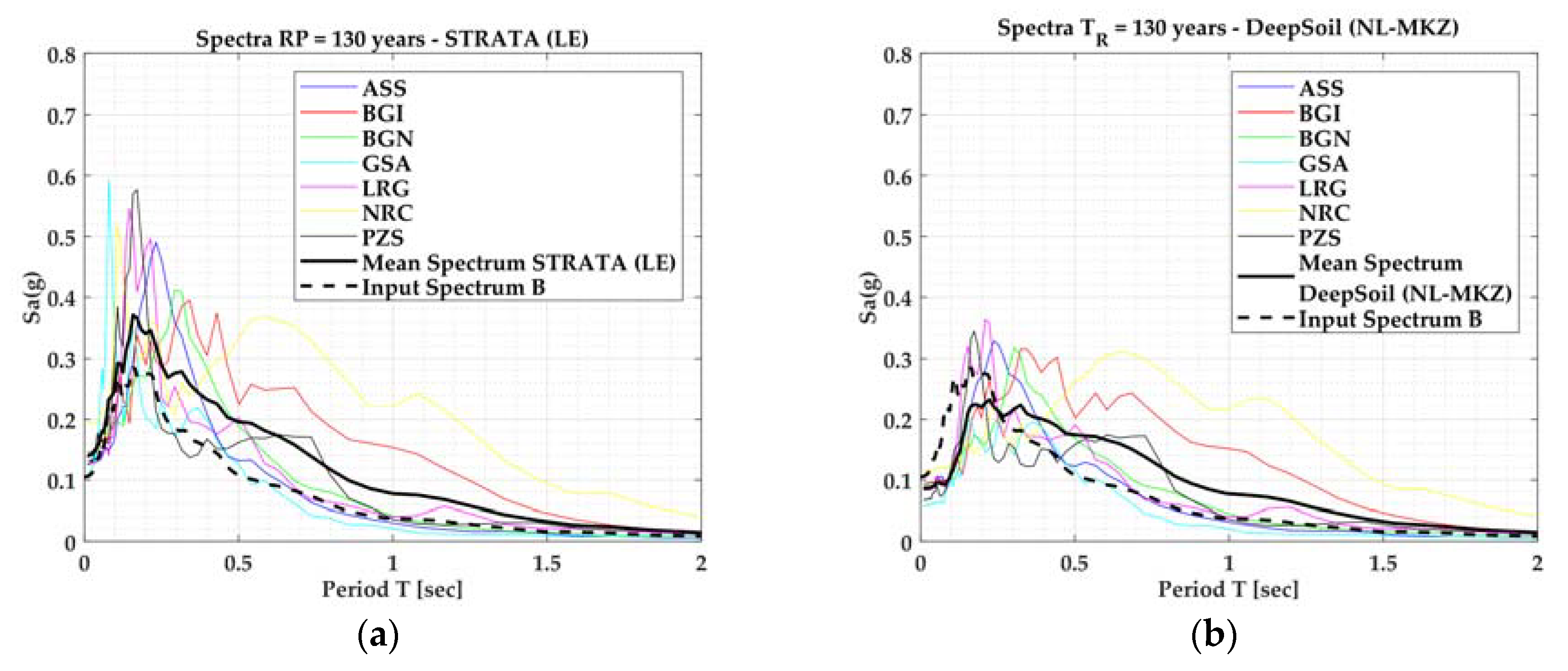
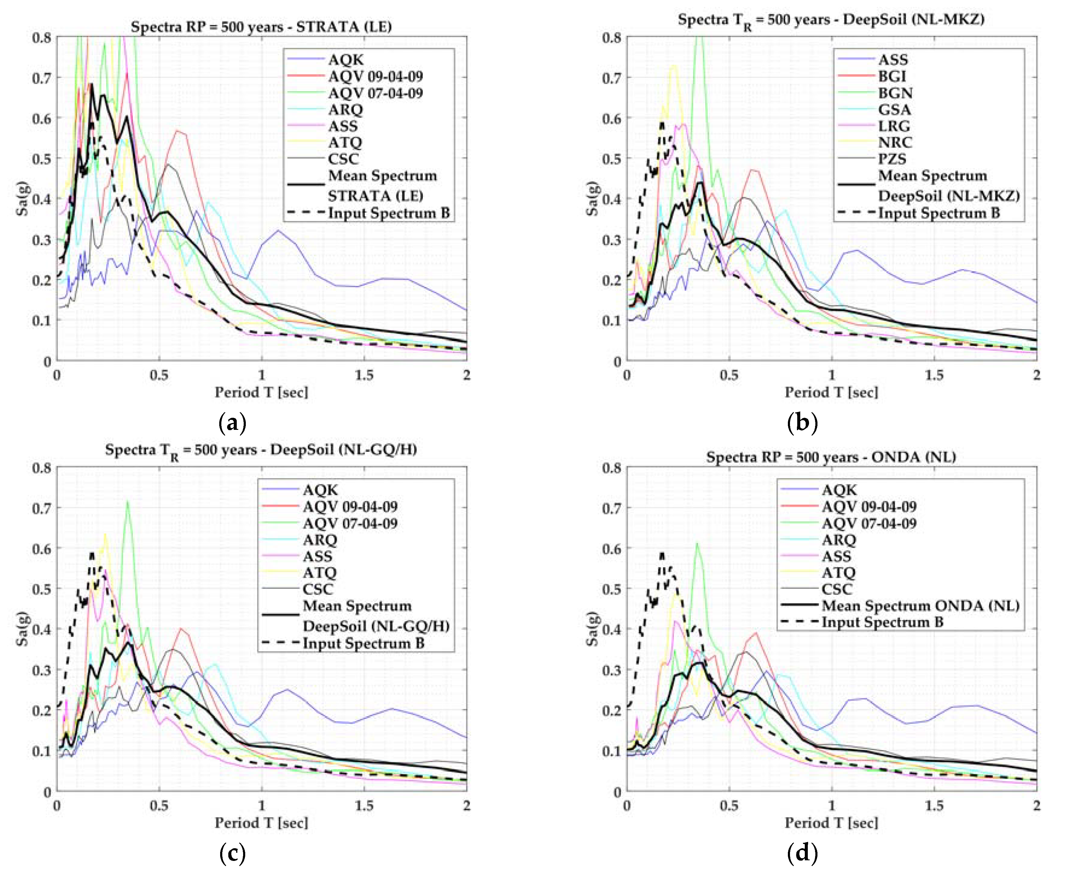
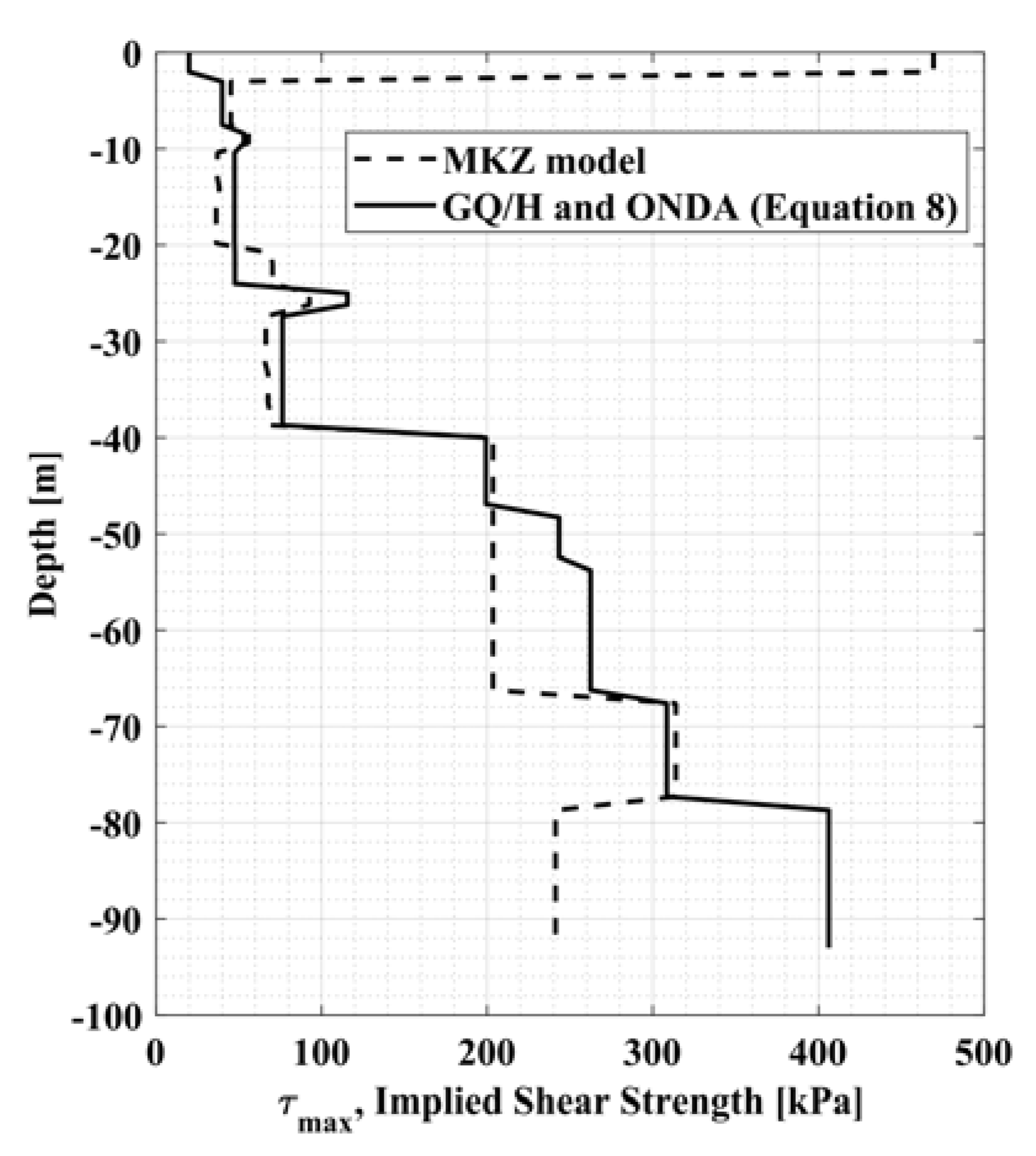
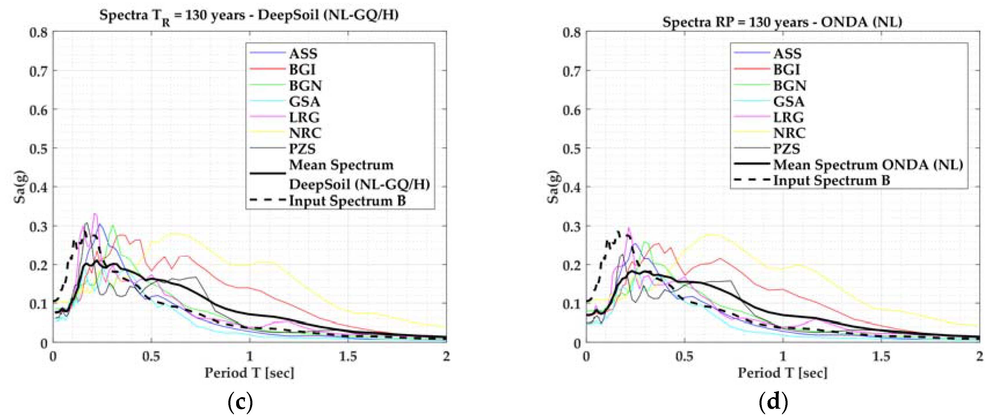
4.3. Seismic Response Analysis Results

Figure 12 shows the difference between the soil shear strength profile obtained with the commonly used MKZ model and that computed with Equation (8), used to perform the nonlinear analyses with strength-controlled constitutive models (DEEPSOIL GQ/H and ONDA).
The MKZ model is not able to correctly reproduce the shear strength profile and largely overestimate the soil resistance at failure down to 4 m in depth, while underestimate the soil resistance at higher depths. This affects the nonlinear soil response analysis results.
The results for a return period of 130 and 500 years are reported in Figure 13 and Figure 14 in terms of horizontal acceleration response spectra computed at ground surface (averaged over all the input motions applied). Average input spectrum at seismic bedrock and amplified spectra are also reported.
Figure 15a,b show the Fourier spectrum ratios between the ground surface and the base of the soil profile for some representative accelerograms at return periods of 130 and 500 years, respectively. In both the Figures and for all the accelerograms, the ratio is generally less than 1 for frequencies above 2 Hz in case of nonlinear analysis.
Figure 16 shows the comparisons between the average response spectra, while Figure 17 the average surface-to-bedrock amplification function for both the return periods considered in this study.
The SRA comparisons shown in Figure 16 and Figure 17 reveal the importance of the selected analysis method (equivalent-linear or nonlinear) in the definition of pseudo-acceleration.
The comparison between equivalent-linear and nonlinear results revealed more evident differences. In fact, equivalent-linear method overestimates the ordinates between 0 and 1.0 s period for 130 years RP, whereas for 500 years RP ordinates are overestimated between 0 and 1.5 s. Maximum overestimation is above 80% in the interval 0–0.5 s.
The equivalent-linear models (e.g., STRATA [28]) consider a single elastic modulus referred to a representative strain level (65% or M-1/10 of the max range).
In nonlinear analyses, on the other hand, the elastic modulus G is updated at each time-step and is reduced considerably for medium-large deformations, causing an increase in the deposit fundamental period and thus shifting the peaks of the spectrum to higher periods.
In the case of 130 years RP above 0.6 s, the nonlinear analyses practically coincide despite the fact that the formulation of the backbone curve adopted in ONDA [32,33] (Ramberg–Osgood) and DEEPSOIL [29] (MKZ [8] and GQ/H [30,31]) is different.
In the case of 500 years RP the differences between the commonly used nonlinear MKZ model and strength-controlled constitutive models (GQ/H and ONDA) become higher compared to seismic motions for 130 years RP. The MKZ model overestimates the ordinates obtained with ONDA of about 10–20% between 0 and 0.8 s. This is due to the different soil modelling for medium-large shear strain levels.
The latter aspect can be clarified showing in Figure 18 the peak shear strain profiles for 130 and 500 years RP seismic motions. In case of 500 years RP acceleration time histories, the attained shear strain levels are larger compared to 130 years RP input motions. For such a reason becomes relevant to consider a strength-controlled constitutive model for the soil response.
This highlights the importance of considering a more proper and realistic soil strength profile in nonlinear analysis methods starting from medium-severe seismic actions.

5. Closing Remarks

The paper shows the results of free-field seismic response analyses (SRA) carried out considering the subsoil of Piazza dei Miracoli in Pisa, where the Leaning Tower is located. Given that this site has been subject to a considerable number of investigations, there is a large number of data available for soil characterization.
The shear wave velocity profile has been recently extended down to more than 100 m below the ground level [6]. One-dimensional SRA were carried out by means of three computer codes: STRATA [28], DEEPSOIL [29] and ONDA [32,33].
The first code performs the analysis in the frequency domain considering an equivalent-linear soil model, whereas DEEPSOIL and ONDA analyze the problem in the time domain assuming true nonlinear soil behavior. All the parameters of the models were calibrated using the same soil data, therefore all three models can be considered as being equivalent.
As discussed in [6], seismic input is affected by some dispersion due to uncertainties related to lack of knowledge. The SRA analyses are also affected by aleatory uncertainty.
The main target of this paper is to show the influence of using new strength-controlled constitutive models in case of 1D nonlinear response analyses. In fact, most of computer codes currently available for nonlinear seismic response analysis use constitutive models able to capture small-strain behavior, but the large-strain shear strength is left uncontrolled. This can affect the assessment of a 1-D response analysis, as in the Pisa subsoil conditions. Nonlinear models seem more appropriate in reproducing the true behavior of the subsoil, however calibrating the parameters seems more difficult.
In this work, differences between the commonly used nonlinear MKZ model and strength-controlled constitutive models (GQ/H and the model implemented in ONDA) are presented. The MKZ model overestimates the pseudo-acceleration values obtained with ONDA and the GQ/H model, especially in case of 500 years RP seismic input motions. This is due to the different soil modelling for medium-large shear strain levels. In fact, the attained shear strain levels are larger compared to 130 years RP acceleration time histories. This reveals the importance to take into account of a proper soil strength profile in nonlinear analysis methods starting from medium-severe seismic actions. Higher differences were found between equivalent-linear and nonlinear codes. The maximum differences between equivalent-linear and nonlinear models are above 80% in both the 130 and 500 years return periods. For RP = 130 years, the differences decrease and become negligible starting from a period approximately equal to 1 s, whereas the differences remain around 40% for RP = 500 years.
The differences among the mean spectra obtained by means of different soil response modelling (equivalent-linear, MKZ model, GQ/H model and ONDA) might be not relevant for a structural designer in case of a new standard building, since it is possible to employ code-defined spectrum or, as an alternative, select the most conservative one.
The selection of the appropriate spectrum assumes particular relevance in case of historical buildings or monuments, because in this case structural interventions have to be respectful of construction integrity and a selection of excessively conservative actions could lead to inappropriate operations [17,42]. Moreover, in the case of the Leaning Tower of Pisa, since the fundamental period is about one second, the uncertainties related to nonlinear models seem negligible with respect to the uncertainty related to seismic input. Further studies and investigations have been planned in order to improve the knowledge of subsoil below 100 m depth. This is expected to improve the capabilities of considered models to forecast the ground response.

Author Contributions

G.F., C.N. and D.L. defined the seismic input motions, N.S. described the subsoil model used to perform the seismic response analyses; S.S. analyzed the RC testing data and performed the seismic response analyses; N.S., G.F. and S.S. wrote the paper.

Acknowledgments

The authors want to thank the Opera della Primaziale Pisana for supporting this research.

Conflicts of Interest

The authors declare no conflict of interest.

References

  1. Squeglia, N.; Bentivoglio, G. Role of Monitoring in Historical Building Restoration: The Case of Leaning Tower of Pisa. Int. J. Archit. Herit. 2015, 9, 38–47. [Google Scholar] [CrossRef]
  2. Burland, J.B.; Jamiolkowski, M.; Viggiani, C. The stabilization of the Leaning Tower of Pisa. Soil. Found. 2003, 43, 63–80. [Google Scholar] [CrossRef]
  3. Macchi, G.; Ghelfi, S. Problemi di consolidamento strutturale. In La Torre Restituita; Settis, A., Ed.; Poligrafico dello Stato: Rome, Italy, 2005. [Google Scholar]
  4. Bartelletti, R.; Fiorentino, G.; Lanzo, G.; Lavorato, D.; Marano, G.C.; Monti, G.; Nuti, C.; Quaranta, G.; Sabetta, F.; Squeglia, N. Behavior of the Leaning Tower of Pisa: Insights on Seismic Input and Soil-Structure Interaction. Appl. Mech. Mater. 2016, 847, 454–462. [Google Scholar] [CrossRef]
  5. Bartelletti, R.; Fiorentino, G.; Lanzo, G.; Lavorato, D.; Marano, G.C.; Monti, G.; Nuti, C.; Quaranta, G.; Sabetta, F.; Squeglia, N. Dynamic Soil Structure interaction of the Leaning Tower of Pisa. In Proceedings of the DISS—Dynamic Interaction of Soil and Structure the 4th International Workshop, Rome, Italy, 12–13 November 2015. [Google Scholar]
  6. Fiorentino, G.; Lavorato, D.; Quaranta, G.; Pagliaroli, A.; Carlucci, G.; Nuti, C.; Sabetta, F.; Della Monica, G.; Piersanti, M.; Lanzo, G.; et al. Numerical and experimental analysis of the leaning Tower of Pisa under earthquake. Procedia Eng. 2017, 199, 3350–3355. [Google Scholar] [CrossRef]
  7. Angina, A.; Steri, A.; Stacul, S.; Lo Presti, D. Free-Field Seismic Response Analysis: The Piazza dei Miracoli in Pisa Case Study. Int. J. Geotech. Earthq. Eng. 2018, 9. [Google Scholar] [CrossRef]
  8. Matasovic, N. Seismic Response of Composite Horizontally-Layered Soil Deposits, Ph.D. Thesis, University of California, Los Angeles, CA, USA, 1993. [Google Scholar]
  9. Consorzio Lamma Geological Maps 100k and 250k. Available online: http://159.213.57.101/geologia/map.phtml?winsize=medium&language=it&config=concessioni (accessed on 12 April 2018).
  10. Regione Toscana Geoscopio. Available online: http://www502.regione.toscana.it/geoscopio/geologia.html (accessed on 12 April 2018).
  11. Viggiani, C.; Pepe, M. Il Sottosuolo della Torre. In La Torre Restituita; Gli studi e gli interventi che hanno consentito la stabilizzazione della Torre di Pisa; Poligrafico dello Stato: Rome, Italy, 2005. [Google Scholar]
  12. Fiorentino, G.; Lavorato, D.; Quaranta, G.; Pagliaroli, A.; Carlucci, G.; Sabetta, F.; Della Monica, G.; Lanzo, G.; Aprile, V.; Marano, G.C.; et al. Leaning Tower of Pisa: Uncertainty reduction for seismic risk assessment through dynamic monitoring, site response analysis and soil-structure interaction modelling. Earthq. Spectra 2018. under review. [Google Scholar]
  13. Grandori, G.; Faccioli, E. Studio per la Definizione del Terremoto di Verifica per le Analisi Sulla Torre di Pisa—Relazione Finale; Comitato per gli interventi di consolidamento e restauro della Torre di Pisa, Incarico Prot: Roman, Italy, 1993. [Google Scholar]
  14. Raptakis, D.; Makra, K. Shear wave velocity structure in western Thessaloniki (Greece) using mainly alternative SPAC method. Soil Dyn. Earthq. Eng. 2010, 30, 202–214. [Google Scholar] [CrossRef]
  15. Rovithis, E.; Kirtas, E.; Bliziotis, D.; Maltezos, E.; Pitilakis, D.; Makra, K.; Savvaidis, A.; Karakostas, C.; Lekidis, V. A LiDAR-aided urban-scale assessment of soil-structure interaction effects: The case of Kalochori residential area (N. Greece). Bull. Earthq. Eng. 2017, 15, 4821–4850. [Google Scholar] [CrossRef]
  16. Progetto INGV-DPC S1 Proseguimento della Assistenza al DPC per il Completamento e la Gestione della Mappa di Pericolosità Sismica Prevista dall’Ordinanza PCM 3274 e Progettazione di Ulteriori Sviluppi. Convenzione INGV-DPC (2004–2006). Task 1—Completamento delle Elaborazion. Available online: http://esse1.mi.ingv.it (accessed on 12 April 2018).
  17. MIBAC. Linee Guida per la Valutazione e Riduzione del Rischio Sismico del Patrimonio Culturale Allineate alle Nuove Norme Tecniche per le Costruzioni (Circolare n.26 2010—Segretariato Generale); Special Recommendation for Cultural Heritage; Ministero dei Beni e delle Attività Culturali e del Turismo: Rome, Italy, 2011; pp. 5–8. (In Italian) [Google Scholar]
  18. Sabetta, F. Seismic hazard and design earthquakes for the central archaeological area of Rome. Bull. Earthq. Eng. 2014, 12, 1307–1317. [Google Scholar] [CrossRef]
  19. Cornell, C.A. Engineering seismic risk analysis. Bull. Seismol. Soc. Am. 1968, 58, 1583–1606. [Google Scholar]
  20. Bazzurro, P.; Allin Cornell, C. Disaggregation of seismic hazard. Bull. Seismol. Soc. Am. 1999, 89, 501–520. [Google Scholar]
  21. Rovida, A.; Locati, M.; Camassi, R.; Lolli, B.; Gasperini, P.; Azzaro, R.; Bernardini, F.; D’Amico, S.; Ercolani, E.; Rossi, A.; et al. CPTI15, the 2015 version of the Parametric Catalogue of Italian Earthquakes. Istituto Nazionale di Geofisica e Vulcanologia. Available online: https://emidius.mi.ingv.it/CPTI15-DBMI15/ (accessed on 12 April 2018).
  22. Akkar, S.; Bommer, J.J. Empirical Equations for the Prediction of PGA, PGV, and Spectral Accelerations in Europe, the Mediterranean Region, and the Middle East. Seismol. Res. Lett. 2010, 81, 195–206. [Google Scholar] [CrossRef]
  23. EN-1998-1. Eurocode 8—Design of Structures for Earthquake Resistance—Part 1: General Rules, Seismic Actions and Rules for Buildings; European Union: Brussels, Belgium, 2004. [Google Scholar]
  24. NTC. Nuove Norme Tecniche per le Costruzioni (DM 14/01/2008); Consiglio Superiore dei Lavori Pubblici: Rome, Italy, 2008. [Google Scholar]
  25. Luzi, L.; Puglia, R.; Russo, E.; D’Amico, M.; Felicetta, C.; Pacor, F.; Lanzano, G.; Çeken, U.; Clinton, J.; Costa, G.; et al. The Engineering Strong-Motion Database: A Platform to Access Pan-European Accelerometric Data. Seismol. Res. Lett. 2016, 87, 987–997. [Google Scholar] [CrossRef]
  26. Rollins, K.M.; Evans, M.D.; Diehl, N.B.; Daily, W.D., III. Shear Modulus and Damping Relationships for Gravels. J. Geotech. Geoenviron. Eng. 1998, 124, 396–405. [Google Scholar] [CrossRef]
  27. Darendeli, M.B. Development of a New Family of Normalized Modulus Reduction and Material Damping Curves. Ph.D. Thesis, The University of Texas at Austin, Austin, TX, USA, 2001. [Google Scholar]
  28. Kottke, A.R.; Rathje, E.M. Technical Manual for Strata; University of Texas: Austin, TX, USA, 2010. [Google Scholar]
  29. Hashash, Y.M.A.; Musgrove, M.I.; Harmon, J.A.; Groholski, D.R.; Phillips, C.A.; Park, D. DEEPSOIL 6.1. User Manual; Board of Trustees of University of Illinois at Urbana-Champaign, Urbana Google Scholar: Springfield, IL, USA, 2016. [Google Scholar]
  30. Groholski, D.R.; Hashash, Y.M.A.; Musgrove, M.; Harmon, J.; Kim, B. Evaluation of 1-D Non-linear Site Response Analysis using a General Quadratic/Hyperbolic Strength-Controlled Constitutive Model. In Proceedings of the 6th International Conference on Earthquake Geotechnical Engineering, Christchurch, New Zealand, 1–4 November 2015. [Google Scholar]
  31. Groholski, D.R.; Hashash, Y.M.A.; Kim, B.; Musgrove, M.; Harmon, J.; Stewart, J.P. Simplified Model for Small-Strain Nonlinearity and Strength in 1D Seismic Site Response Analysis Supplement Data. J. Geotech. Geoenviron. Eng. 2016, 142, 4016042. [Google Scholar] [CrossRef]
  32. Lo Presti, D.C.; Lai, C.G.; Puci, I. ONDA: Computer Code for Nonlinear Seismic Response Analyses of Soil Deposits. J. Geotech. Geoenviron. Eng. 2006, 132, 223–236. [Google Scholar] [CrossRef]
  33. Lo Presti, D.; Stacul, S. ONDA (One-dimensional Non-linear Dynamic Analysis): ONDA 1.4 User’s Manual Version 1.4. Available online: http://doi.org/10.13140/RG.2.2.32409.83043 (accessed on 12 April 2018).
  34. Idriss, I.M.; Sun, J.I. SHAKE91: A Computer Program for Conducting Equivalent Linear Seismic Response Analyses of Horizontally Layered Soil Deposits; University of California: Oakland, CA, USA, 1992. [Google Scholar]
  35. Chopra, A.K. Dynamics of Structures; Prentice Hall: Upper Saddle River, NJ, USA, 1995. [Google Scholar]
  36. Newmark, N.M. A Method of Computation for Structural Dynamics. J. Eng. Mech. Div. 1959, 85, 67–94. [Google Scholar]
  37. Ramberg, W.; Osgood, W.R. Description of Stress-Strain Curves by Three Parameters; National Advisory Committee for Aeronautics: Washington, DC, USA, 1943. [Google Scholar]
  38. Hardin, B.O.; Drnevich, V.P. Shear Modulus and Damping in Soils. J. Soil Mech. Found. Div. 1972, 98, 667–692. [Google Scholar]
  39. Masing, G. Eigenspannungen und Verfestigung beim Messing. In Proceedings of the 2nd International Congress of Applied Mechanics, Zürich, Switzerland, 12–17 September 1926. [Google Scholar]
  40. Tatsuoka, F.; Siddique, M.S.A.; Park, C.S.; Sakamoto, M.; Abe, F. Modelling stress-strain relations of sand. Soils Found. 1993, 33, 60–81. [Google Scholar] [CrossRef]
  41. Camelliti, A. Influenza dei Parametri del Terreno sulla Risposta Sismica dei Depositi. Ph.D. Thesis, Technical University of Turin, Department of Structural and Geotechnical Engineering, Turin, Italy, 1999. [Google Scholar]
  42. Squeglia, N.; Stacul, S.; Diddi, E. The restoration of San Paolo Church in Pisa: Geotechnical aspects. Riv. Ital. Geotec. 2015, 49, 58–69. [Google Scholar]
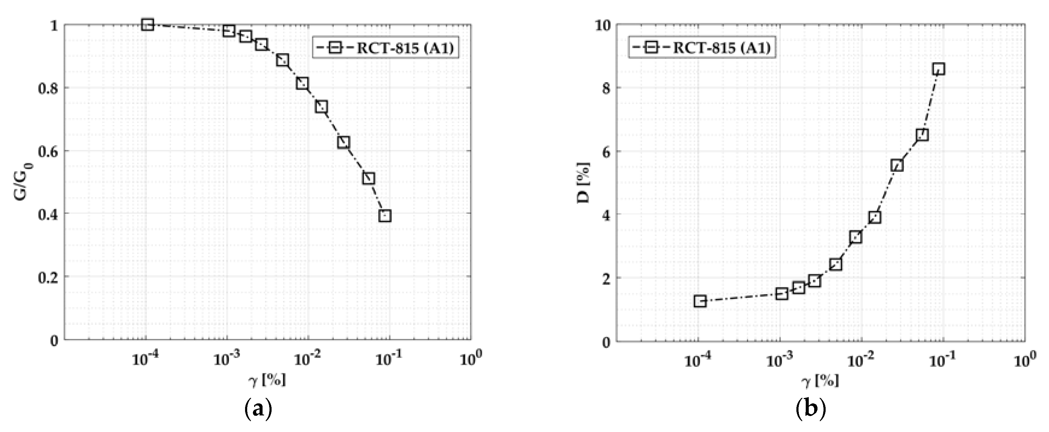
Figure 1. Geological map of the study area. (Adapted from: Consorzio Lamma Database [9]).
Geosciences 08 00228 g001
Figure 2. Morphological map of the study area. The scale is the same as the previous figure. (Adapted from: Tuscany Region Database–Geoscopio [10]).
Geosciences 08 00228 g002
Figure 3. The subsoil of the Tower. (After Viggiani and Pepe, 2005 [11]).
Geosciences 08 00228 g003
Figure 4. Water head in Horizon A (3), intermediate sand (2) and lower sand (1). (After Viggiani and Pepe, 2005 [11]).
Geosciences 08 00228 g004
Figure 5. Profile of the shear wave velocity.
Geosciences 08 00228 g005
Figure 6. Time histories of the scaled accelerograms for an RP of 130 years.
Geosciences 08 00228 g006
Figure 7. Time histories of the scaled accelerograms for an RP of 500 years.
Geosciences 08 00228 g007
Figure 8. Average response spectrum. Spectrum-compatibility is assumed between 0.3–1.1 s. (a) Return period = 130 years; (b) return period = 500 years.
Geosciences 08 00228 g008
Figure 9. Resonant column test (RCT-815; 815 is the registration number of the soil sample) results (lithotype A1): (a) modulus reduction curve; (b) damping ratio.
Geosciences 08 00228 g009
Figure 10. Comparison between the experimental and the adopted: (a) modulus reduction curve; (b) damping ratio curve (lithotype A1).
Geosciences 08 00228 g010
Figure 11. Comparison between the experimental and the adopted: (a) modulus reduction curve; (b) damping ratio curve (Upper Pancone). In this Figure, triangles represent the best-fit of the collected experimental data related to the Upper Pancone as reported in [7].
Geosciences 08 00228 g011
Figure 12. Implied shear strength profiles.
Geosciences 08 00228 g012
Figure 13. Results of SRA for return period = 130 years with: (a) STRATA (LE); (b) DEEPSOIL (NL-MKZ); (c) DEEPSOIL (NL-GQ/H); (d) ONDA (NL).
Geosciences 08 00228 g013aGeosciences 08 00228 g013b
Figure 14. Results of SRA for return period = 500 years with: (a) STRATA (LE); (b) DEEPSOIL (NL-MKZ); (c) DEEPSOIL (NL-GQ/H); (d) ONDA (NL).
Geosciences 08 00228 g014
Figure 15. Fourier spectrum ratios between the surface and the base of the soil profile for some relevant input motions: (a) return period = 130 years; (b) return period = 500 years.
Geosciences 08 00228 g015
Figure 16. Comparison between results of different SRA analyses: (a) RP = 130 years; (b) RP = 500 years.
Geosciences 08 00228 g016
Figure 17. Average surface-to-bedrock amplification function: (a) RP = 130 years; (b) RP = 500 years.
Geosciences 08 00228 g017
Figure 18. Comparison between the peak shear strain profiles using different SRA analyses: (a) RP = 130 years–input motion GSA; (b) RP = 500 years–input motion AQK.
Geosciences 08 00228 g018
Table 1. Subsoil model adopted for site response analysis.
Hor.LayerUSCS Class.ΔH (m)K0 (-)OCR (-)PI (%)φ (°)c‘ (kPa)U.W. (kN/m3)Vs (m/s)G/G0 & D-γ Curves
MGMG-3.0-----18.50 ± 0.80180[26] Average curve
AA1ML5.41.053.513346.818.86 ± 0.72180RC Test (2016)
A2SC-SM2.00.882.530346.818.07 ± 0.85180[27]-PI = 30,
σ‘v = 0.55 bar
BB1CH3.50.62243262.417.00 ± 0.89180RC tests
B2CH2.00.541.533267.717.49 ± 0.57180RC tests
B3CH4.90.421.5412015.916.67 ± 0.58180RC tests
B4CH1.20.611.53330019.48 ± 0.96230RC tests
B5CL3.00.611.52330019.76 ± 0.79230RC tests
B6SC-SM2.40.882.5834019.11 ± 0.49230[27]-PI = 8,
σ‘v = 2.0 bar
B7CH4.60.541.534263.118.62 ± 0.97230RC tests
B8CL1.40.541.523263.118.41 ± 0.51230RC tests
B9CH4.00.541.531263.119.01 ± 1.41230RC tests
B10CH2.60.541.529263.119.38 ± 0.44230RC tests
CC1SC-SM27.6-----20.52 ± 1.29340[27]-PI = 0,
σ‘v = 3.50 bar
C2-11.1--15---340[27]-PI = 15,
σ‘v = 5.0 bar
C3-16.3------340[27]-PI = 0,
σ‘v = 6.0 bar
Bedrock (C3) ------21.00500-
Hor. = horizon; ΔH = layer thickness; K0 = at-rest earth pressure coefficient; OCR = overconsolidation ratio; PI = plasticity index; φ = angle of friction; c’ = effective cohesion; U.W. = soil unit weight; Vs = shear wave velocity, G/G0 = normalized secant shear modulus; D = damping ratio; γ = shear.

