Simulating the Influence of Buildings on Flood Inundation in Urban Areas

Abstract

Two-dimensional hydraulic modeling is fundamental to simulate flood events in urban area. Key factors to reach optimal results are detailed information about domain geometry and utility of hydrodynamic models to integrate the full or simplified Saint Venant equations in complex geometry. However, in some cases, detailed topographic datasets that represent the domain geometry are not available, so approximations—such as diffusive wave equation—is introduced whilst representing urban area with an adjusted roughness coefficient. In the present paper, different methods to represent buildings and approximation of the Saint Venant equations are tested by performing experiments on a scale physical model of urban district in laboratory. Simplified methods are tested for simulation of a real flood event which occurred in 2013 in the city of Olbia, Italy. Results show that accuracy of simulating flow depth with a detailed geometry is comparable to the one achieved with an adjusted roughness coefficient.

1. Introduction

Flood events are one of the most dangerous natural phenomena connected to human activities, with possible consequences on people’s safety and economic losses [1].

The flood hazard affecting densely populated areas is increasing in recent times, due to the intensification of extreme meteorological events and poorly managed urban development [2]. Two-dimensional flood inundation modeling is a pivotal component of flood risk assessment and management. It is therefore not surprising that over the last few decades significant efforts have been devoted to the development of increasingly complex algorithms to simulate the flow of water in streams and floodplains [3,4,5,6,7,8,9,10]. In areas with mild slope terrain, one-dimensional models may produce misleading results and two-dimensional (2D) models are recommended also for their ability to capture preferential flow directions caused by the presence of buildings [11,12].

The correct representation of buildings in a 2D model is a fundamental factor to reach good flood simulation results in urban areas. When detailed geometry is available, the individual shapes of buildings can be incorporated into the calculations. For large scale modeling or when detailed geometry information are not available, flow obstructions may be represented as areas with higher roughness coefficient (roughness approach). This accounts for the increased resistance induced by the presence of buildings in the urban area. Moreover, low accuracy of available topographic data justifies introducing some simplifications to the Saint Venant equations, also known as shallow water equations (SWE), that describe fluid dynamics [13,14,15]. In most practical applications of flood simulation, the diffusive wave simplification is preferred to the full solution (dynamic wave), since the local and convective acceleration terms are small in comparison to the bed slope [16].

In the last few decades, many aspects of urban flooding have been investigated through experimental studies [17,18], and few of these investigations have focused on how to properly represent buildings within inundation models [19,20].

The main objective of this paper is to verify the accuracy of the roughness approach against full buildings incorporation in flood simulation. Further analysis was dedicated to test diffusive model against full SVE. The novelty of this research is that three different methods to represent buildings are tested by performing a number of laboratory experiments carried out with a simplified urban district physical model, and reconstructing results with a hydraulic mathematical model considering both the solution of the full SWE and the diffusive simplification. Simplified methods are tested for simulation of a real flood event that hit the city of Olbia, Italy, on November 2013.

2. Materials and Methods

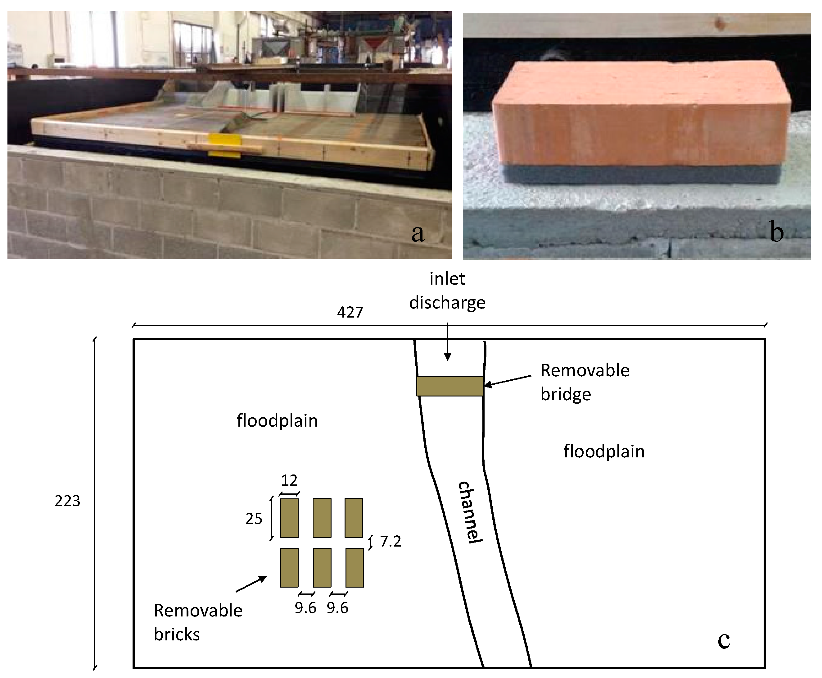
2.1. Experimental Setup

Experiments were performed on a physical scale model at the Fantoli Hydraulic Laboratory at the Politecnico di Milano (Figure 1a). The model was implemented for verifying the hydraulic performance of the dam body of an on-stream detention basin designed for flood risk reduction of the Fosso di Pratolungo river, a small tributary of the river Aniene, in the Lazio region, Italy. Flow into the physical model is regulated by two triangular Thompson weirs, often used in laboratory experiments for their high sensitivity to low flow rates. The maximum flow rate achievable, is 110 L/s. The ratio between the physical model lengths and the prototype is 1:25. Specifically for this work, we considered the channel reach and floodplain downstream of the dam artifact (427 cm × 223 cm), where six bricks (12 cm × 25 cm) were placed for the representation of a small urban area with regular simple geometry (Figure 1c). An impermeable foam layer was attached to the lower side of the bricks in order to follow the irregularities of floodplain reproduced in the physical model (Figure 1b). A removable bridge was placed within the channel (Figure 1c) and the channel end was blocked with a board (Figure 1a) in order to promote floodplain inundation.

Water level and velocity were measured using a portable high precision nonius hydrometric rod and a micro-current-meter, respectively, in the points shown in Figure 2. The hydrometric rod was used to measure floodplain and channel bed elevation with a spatial resolution of 1 cm, leading to the digital elevation model shown in Figure 2.

2.2. Mathematical Hydraulic Modelling

In order to simulate the flood inundation, the Hec-Ras model was employed [21]. As from release 5.0, Hec-Ras is designed to simulate one-dimensional, two-dimensional, and combined one/two-dimensional unsteady flow through a full network of open channels, floodplains, and alluvial fans. For the purpose of this work, flood inundation was simulated with unsteady two-dimensional solution of the full SWE and the simplified diffusive equation. When a steady state was required, this was reached by setting as input a constant discharge hydrograph long enough to reach the steady condition.

Several methods have been proposed to set the friction coefficient when roughness approach is employed to simulate flow obstacles such as the equivalent friction slope method [22,23] or similar methods [24]. In this work, we chose to use roughness Manning coefficient reported in the Hec-Ras 2D manual [25] as this is what is likely done for practical engineering applications. Further analysis to verify possible improvement when using different approaches to set roughness coefficient is ongoing.

Buildings were modeled in three different ways:

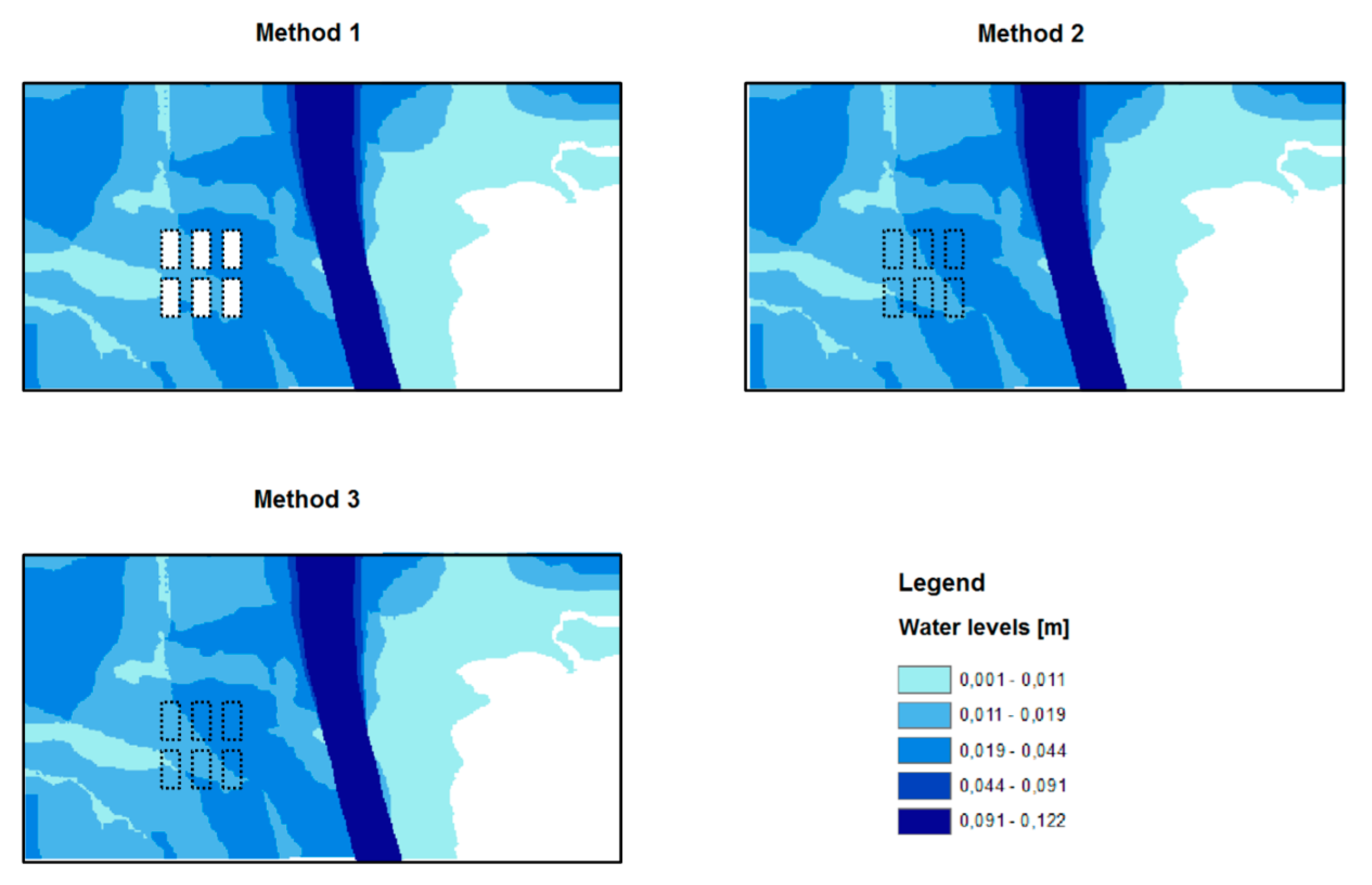
• Method 1: incorporation of buildings using the detailed digital elevation model (DEM) with 1 cm spatial resolution.
• Method 2: buildings are replaced by a flat area with high roughness (Manning coefficient = 10).
• Method 3: all urban area is replaced by a flat area with high roughness (Manning coefficient = 0.15).

The mean relative absolute error (MRAE) was computed as goodness of fit index

$$MRAE=\frac{{{\displaystyle \sum }}_{i=1}^n\left|X_{obs,i}-X_{mod,i}\right|/X_{obs,i}}{n}$$

(1)

where X_obs and X_mod are the observed and modeled values, respectively, n is the number of points compared.

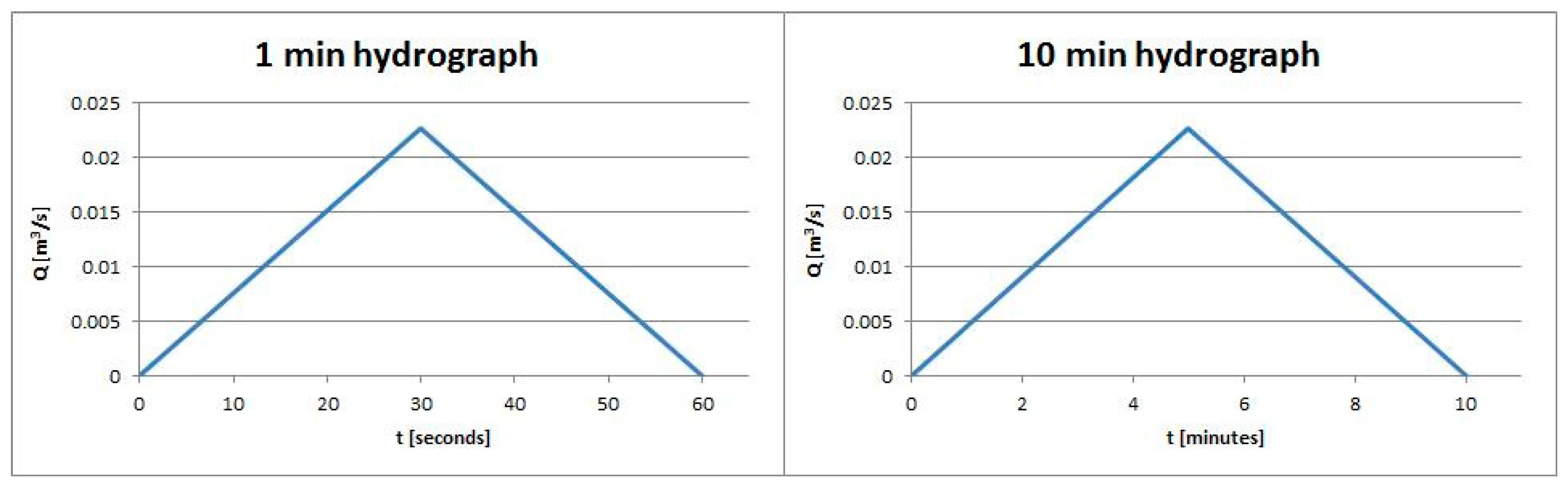
2.3. Hydrologic Model

Flood hydrograph of the six streams flowing to Olbia during the 2013 flood were simulated with the FEST model (flash-flood event-based spatially distributed rainfall-runoff transformation) [26,27,28,29]. FEST is a distributed, raster-based hydrologic model developed focusing on flash-flood event simulation. As a distributed model, FEST can manage spatial distribution of meteorological forcings, and heterogeneity in hill slope and drainage network morphology (slope, roughness, etc.) and land use.

The FEST model has three principal components. In the first component, the flow path network is automatically derived from the digital elevation model using a least-cost path algorithm [30]. In the second component, the surface runoff is computed for each elementary cell using the SCS-CN method [31,32]. The third component performs the runoff routing throughout the hill slope and the river network through a diffusion wave scheme based on the Muskingum–Cunge method in its non-linear form with the time variable celerity [33]. Spatial resolution of input maps was 10 m.

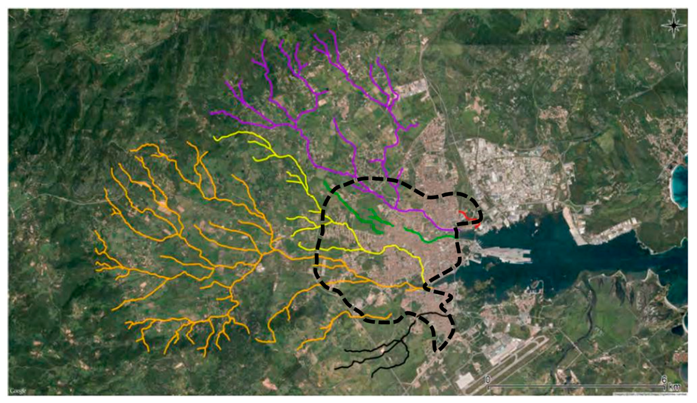
2.4. The 2013 Flood in Olbia

Olbia is a flood-prone city located in Sardinia, Italy, that developed in an alluvial plain bounded on the West side by a steep mountains chain and on the East side by the Tyrrhenian Sea. Six creeks cross this area with drainage area ranging from 0.5 km² to 38.4 km² (Figure 3). A steep slope in the upper part and a mild slope in the valley where city mostly expanded characterize them.

The peculiar morphology of the territory together with the urbanization pressure have contributed to transform a flood prone area into a high flood risk territory demonstrated by catastrophic floods that hit Olbia in 1970, 2013, and 2015.

Specifically, on 18 November 2013, the island of Sardinia (Italy) was affected by a meteorological event, named Cleopatra, characterized by extreme rainfall intensity (rain rate exceeded 120 mm/h in some localities), and amount (more than 450 mm of cumulated rainfall in 15 h) that sets the maximum return period of precipitation well above 200 years. Continuous rain over two days resulted in the overflowing of the rivers in the north-eastern part of Sardinia. Olbia was one of the affected cities of the island, with discharge values that reached the 25-year return period. Images and videos of the flood can be seen on the page dedicated by BBC to the Cleopatra cyclone affecting Sardinia (http://www.bbc.com/news/world-europe-24996292).

After the flood, the technical office of the Municipality carried out a survey of the flooded areas in the urban center of Olbia.

3. Results

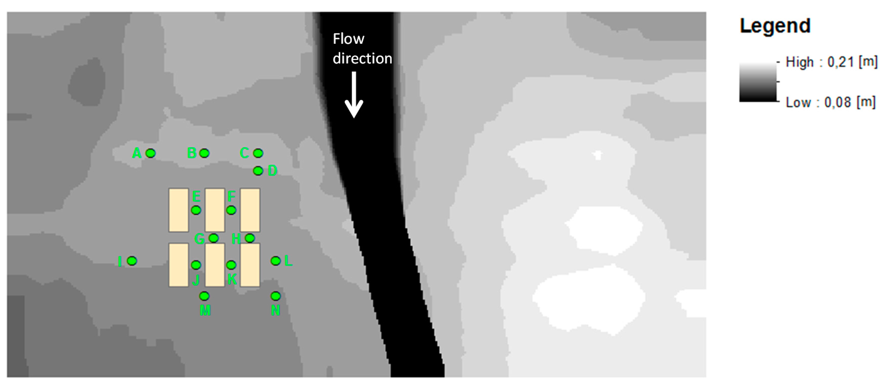
3.1. Simulation of Flow Depth and Velocity of the Laboratory Experiments

The first phase of experiments was dedicated to calibrate the Manning roughness coefficient of the channel and the floodplains. In this phase, bricks and bridge were removed from the physical model. Normal depth was set as boundary condition on domain border. The domain was implemented with a square mesh with 1 cm spatial resolution.

Measurements of the free-surface profile in the channel and over the floodplain for various flow rates (15, 18, and 21 L/s) were compared to values computed with Hec-Ras with different roughness coefficient. The roughness coefficient value that minimized the difference between measured and computed water profile was 0.0166 s m^−1/3, which is in consistent with the expected value for concrete.

In the second phase, the bricks and bridge were positioned in the model, and experiments were performed considering a constant flow rate of 22.6 L/s, discharged through the dam bottom spillway of the physical model. Flow depth and velocity measured values were compared to mathematical model simulation results obtained with the solution of the diffusive equation and considering the three methods for representing buildings described in Section 2.2. Simulated water levels and velocities are shown in Figure 4 and Figure 5, respectively.

In

Table 1. Observed and simulated water levels with Methods 1, 2, and 3.

Point	Observed Water Level (m)	Simulated Water Level (m)
		Method 1	Method 2	Method 3
A	0.014	0.009	0.009	0.009
B	0.022	0.014	0.013	0.014
C	0.022	0.016	0.016	0.016
D	0.044	0.024	0.023	0.024
E	0.015	0.019	0.019	0.019
F	0.021	0.021	0.021	0.022
G	0.016	0.018	0.019	0.019
H	0.024	0.022	0.021	0.022
I	0.011	0.008	0.009	0.009
J	0.010	0.014	0.014	0.014
K	0.017	0.018	0.018	0.018
L	0.040	0.023	0.022	0.022
M	0.019	0.019	0.019	0.019
N	0.044	0.027	0.026	0.026

and

Table 2. Observed and simulated water velocities with Methods 1, 2, and 3.

Point	Observed Water Velocity (m/s)	Simulated Water Velocity (m/s)
		Method 1	Method 2	Method 3
A	0.505	0.345	0.331	0.351
B	0.416	0.392	0.370	0.369
C	0.862	0.340	0.355	0.341
D	0.590	0.373	0.368	0.349
E	0.359	0.400	0.350	0.072
F	0.497	0.400	0.330	0.058
G	0.267	0.103	0.442	0.078
H	0.267	0.117	0.450	0.072
I	NA	0.412	0.459	0.440
J	0.382	0.490	0.530	0.086
K	0.566	0.550	0.550	0.092
L	0.673	0.526	0.515	0.546
M	0.244	0.390	0.416	0.432
N	0.659	0.700	0.680	0.687

Note: NA = measure was not possible

observed and simulated water level and velocity, respectively, the 14 points monitored are reported. MRAE and standard deviation values computed between observed and simulated water levels and velocities are reported in

Table 3. Mean relative absolute error, with standard deviation in brackets, for water level and velocity simulation with the three different methods.

	Method 1	Method 2	Method 3
Level	0.248 (0.157)	0.257 (0.161)	0.252 (0.154)
Velocity	0.309 (0.214)	0.347 (0.244)	0.551 (0.288)

. Errors related to water levels are lower than values calculated for water velocity; this is probably also justified by the relatively higher uncertainty intrinsically involved in the velocity measuring in very low water depth (indeed, in point I, it was not possible to get velocity measurement).

As a general comment, the three methods tested are all equivalent in simulating water depths, while Method 3 is not able to correctly capture water velocities within the area approximated with a homogeneous roughness coefficient. In fact, velocity computed inside the buildings (points E, F, G, H, J, and K) do not have a physical meaning when Method 3 is used. Method 3 is intended for considering effect of urban area on flood inundating surrounding places and not to investigate flow dynamics inside the urban area.

In Method 2 and 3, as buildings that are considered impervious in Method 1 are represented only with a different roughness coefficient, water is free to flow in the area occupied by buildings, although with velocities close to zero. While this does not represent an issue when performing constant flow rate simulations, it could introduce error in inundation volume when simulating unsteady flow transient condition with discharge changing over time.

For this reason, further simulations for Methods 1 and 2 were performed, considering two different triangular symmetric hydrographs characterized by the same peak discharge, and two different durations, 1 and 10 min (denoted H1 and H10, respectively), so to consider two hydrographs with different volume (Figure 6). Moreover, water flow was also simulated running full SWE, to evaluate possible differences against simplified diffusive scheme. As the laboratory model was not intended for reproducing unsteady hydrograph, in this test we could only compare simulated data. The goodness of fit indexes are to be interpreted as the deviation of Method 2 with respect to the Method 1 simulation. Water depth and velocity in points F, G, and J are considered in this analysis at 20, 40, and 60 s for H1, and 3, 6, and 10 min for H10.

The results shown in

Table 4. Mean relative absolute deviation of Method 2 respect to Method 1 in reconstructing water levels and velocities with 1 min (H1) and 10 min (H10) duration hydrographs.

	Water Levels		Water Velocities
Simulation	Diffusive	Dynamic	Diffusive	Dynamic
H1	0.04	0.11	0.64	0.27
H10	0.04	0.09	0.71	0.22

confirm small differences between Methods 1 and 2 concerning water levels, especially using diffusive model, with a maximum deviation of 0.11 when full SWE are solved with H1. This confirms that the roughness approach and diffusive solution of SWE are good enough to simulate water depths even with unsteady flow hydrographs.

On the other hand, by analyzing water velocities, greater differences between Method 1 and 2 are reported for both the simulations, especially for the diffusive model.

Finally, an advantage of the diffusive solution is that it is faster than full SWE; in particular, the simplified simulation took about 20% time less than the full solution on a laptop computer with 1.5 GHz CPU clock speed and 2 GB ram.

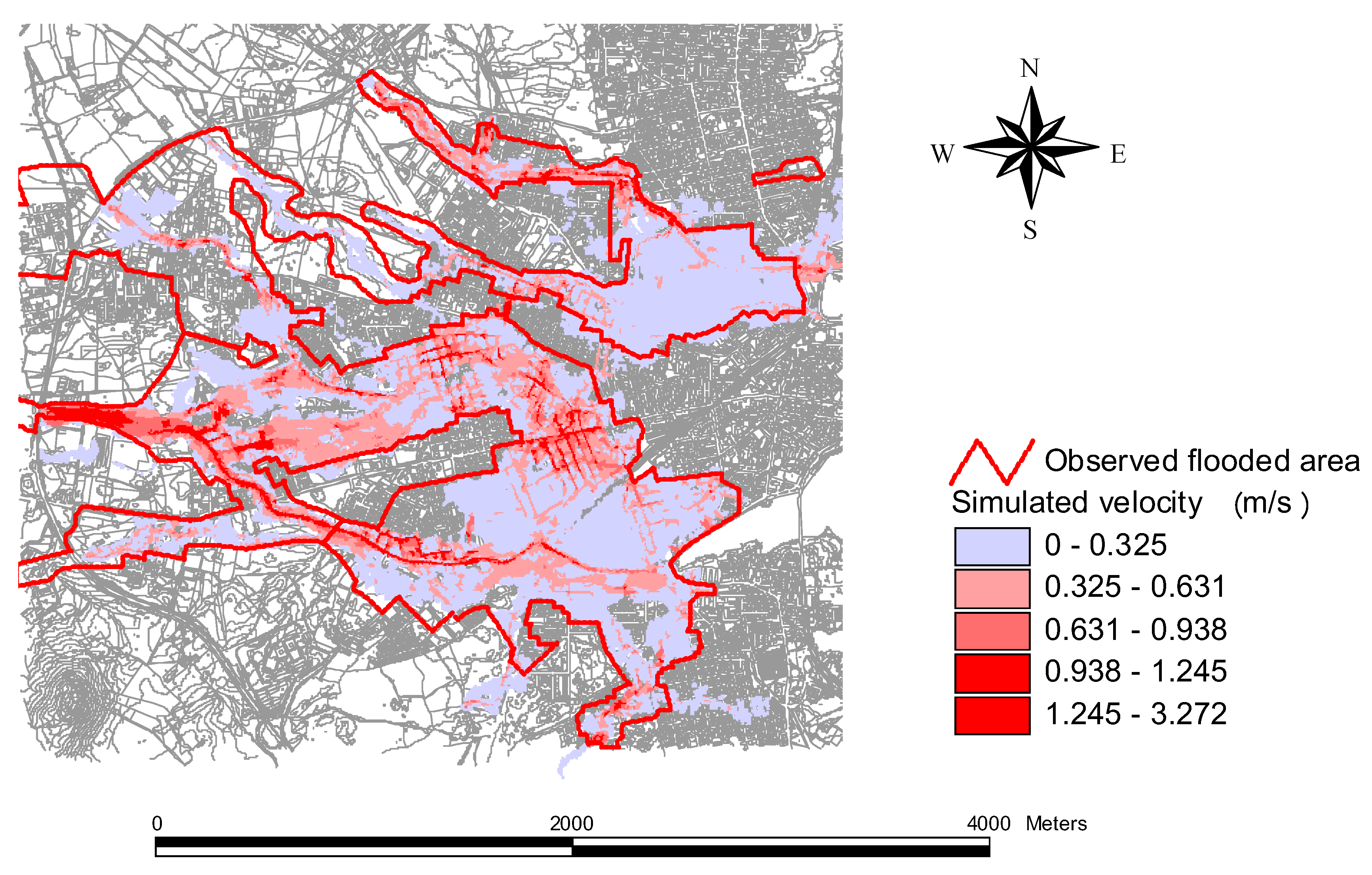
3.2. Simulation of Olbia Flood Inundation

Results presented in the previous section show that Methods 1 and 2 provide similar accuracy in simulating water depth and velocity in urban area. This is relevant when one flood event has to be simulated in an urban area for which detailed buildings geometry is not available. In order to validate these findings, the 2013 flood that occurred in Olbia was simulated with the assumptions of Method 2, that are 2D diffusive solution model and buildings represented with high roughness cells (Manning coefficient = 10). Method 1 could not be applied as available DEM does not include building geometry, only terrain elevation is provided. Method 3 was not applied as it is assumed to be more suited to flood simulation over larger areas with many urbanized zones in them. In the case of the Olbia flood, we are interested in reconstructing detailed inundation in one single urban area.

Hydrographs of the six streams flowing to Olbia reconstructed by the FEST hydrological model were used as forcing input of the hydraulic model. The domain was implemented with a square mesh with 15 m spatial resolution deriving information from an available LIDAR survey with 1 m spatial resolution.

By comparing the flood extent simulated by the hydraulic model and the one surveyed after the flood (Figure 7 and Figure 8), a good agreement can be observed. The small discrepancy is probably due to the contribution of the subsurface urban drainage flow that is not considered in the mathematical model, and uncertainties in hydrological reconstruction of stream flood hydrographs. This confirms that the use of a simplified equation and approximation of buildings as high friction cells does not introduce significant error in practical applications when flood area must be assessed, even in a complex area such as the one considered in this analysis.

4. Conclusions

In this paper, three different methods to simulate the influence of buildings on flood inundation have been tested against measurement undertaken on a simplified urban district model in laboratory. The first method considered detailed information about topography of area containing the buildings. According to the further two methods tested, single buildings or the entire urban district are represented with a high friction area.

Results show that adoption of 2D diffusive model and roughness parameter method to represent buildings is a good option to model water heights, even when unsteady discharge with rapid change in time is considered.

On the other hand, water velocities are significantly better reconstructed by methods that consider the effect of single buildings, like in Methods 1 and 2. Results of unsteady analysis show that solution of the full SWE is less sensitive to the method considered for representing buildings respect to diffusive simplification.

Application to the simulation of a real flood that occurred in Olbia (Italy) demonstrated that use of 2D diffusive model and setting high friction instead of detailed building geometry is an effective method to assess flood inundation extent.

References

1. Berz, G.; Kron, W.; Loster, T.; Rauch, E.; Schimetschek, J.; Schmieder, J.; Siebert, A.; Smolka, A.; Wirtz, A. World map of natural hazards—A global view of the distribution and intensity of significant exposures. Nat. Hazards 2001, 23, 443–465. [Google Scholar] [CrossRef]
2. Milly, P.C.D.; Wetherald, R.T.; Dunne, K.A.; Delworth, T.L. Increasing risk of great floods in a changing climate. Nature 2002, 415, 514–517. [Google Scholar] [CrossRef] [PubMed]
3. De Almeida, G.A.M.; Bates, P.; Freer, J.; Souvignet, M. Improving the stability of a simple formulation of the shallow water equations for 2-D flood modeling. Water Resour. Res. 2012, 48, W05528. [Google Scholar] [CrossRef]
4. Peraire, J.; Zienkiewicz, O.C.; Morgan, K. Shallow water problems: a general explicit formulation. Int. J. Numer. Methods Eng. 1986, 22, 547–574. [Google Scholar] [CrossRef]
5. Toro, E.F.; Garcia-Navarro, P. Godunov-type methods for freesurface shallow flows: A review. J. Hydraul. Res. 2007, 45, 736–751. [Google Scholar] [CrossRef]
6. Guinot, V.; Frazão, S. Flux and source term discretization in two-dimensional shallow water models with porosity on unstructured grids. Int. J. Numer. Method Fluids 2006, 50, 309–345. [Google Scholar] [CrossRef]
7. LeVeque, R.J.; George, D.L. High-resolution finite volume methods for the shallow water equations with bathymetry and dry states. In Advanced Numerical Models for Simulating Tsunami Waves and Runup; World Scientific: Singapore, 2008; Available online: http://www.amath.washington.edu/rjl/pubs/catalina04 (accessed on 10 January 2018).
8. Sanders, B.; Schubert, J.E.; Gallegos, H.A. Integral formulation of shallow-water equations with anisotropic porosity for urban flood modeling. J. Hydrol. 2008, 362, 19–38. [Google Scholar] [CrossRef]
9. Li, S.; Duffy, C.J. Fully coupled approach to modeling shallow water flow, sediment transport, and bed evolution in rivers. Water Resour. Res. 2011, 47, W03508. [Google Scholar] [CrossRef]
10. Tsakiris, G. Flood risk assessment: Concepts, modelling, applications. Nat. Hazard Earth Syst. Sci. 2014, 14, 1361–1369. [Google Scholar] [CrossRef]
11. Alcrudo, F. Mathematical Modelling Techniques for Flood Propagation in Urban Areas. IMPACT Project Technical Report. Available online: http://www.impact-project.net/AnnexII_DetailedTechnicalReports/AnnexII_PartB_WP3/Modelling_techniques_for_urban_flooding.pdf (accessed on 10 January 2018).
12. Liu, L.; Liu, Y.; Wang, X.; Yu, D.; Liu, K.; Huang, H.; Hu, G. Developing an effective 2-D urban flood inundation model for city emergency management based on cellular automata. Nat. Hazards Earth Syst. Sci. 2015, 15, 381–391. [Google Scholar] [CrossRef] [Green Version]
13. Dottori, F.; Todini, E. Testing a simple 2D hydraulic model in an urban flood experiment. Hydrol. Proces. 2013, 27, 1301–1320. [Google Scholar] [CrossRef]
14. McMillan, H.K.; Brasington, J. Reduced complexity strategies for modelling urban floodplain inundation. Geomorphology 2007, 90, 226–243. [Google Scholar] [CrossRef]
15. Hunter, N.M.; Bates, P.D.; Horritt, M.S.; Wilson, M.D. Simple spatially distributed models for predicting flood inundation: A review. Geomorphology 2007, 90, 208–225. [Google Scholar] [CrossRef]
16. Prestininzi, P. Suitability of the diffusive model for dam break simulation: Application to a CADAM experiment. J. Hydrol. 2008, 361, 172–185. [Google Scholar] [CrossRef]
17. Lopes, P.; Leandro, J.; Carvalho, R.F.; Páscoa, P.; Martins, R. Numerical and experimental investigation of a gully under surcharge conditions. Urban Water J. 2015, 12, 468–476. [Google Scholar] [CrossRef]
18. Bazin, P.-H.; Nakagawa, H.; Kawaike, K.; Paquier, A.; Mignot, E. Modeling flow exchanges between a street and an underground drainage pipe during urban floods. J. Hydraul. Eng. 2014, 140, 4014051. [Google Scholar] [CrossRef]
19. Zhou, Q.; Yu, W.; Chen, A.S.; Jiang, C.; Fu, G. Experimental assessment of building blockage effects in a simplified urban district. Procedia Eng. 2016, 154, 844–852. [Google Scholar] [CrossRef]
20. Testa, G.; Zuccala, D.; Alcrudo, F.; Mulet, J.; Soares-Frazão, S. Flash flood flow experiment in a simplified urban district. J. Hydraul. Res. 2007, 45, 37–44. [Google Scholar] [CrossRef]
21. US Army Corps of Engineers—Hydrologic Engineering Center. Hydraulic Reference Manual. Available online: http://www.hec.usace.army.mil/software/hec-ras/documentation/HEC-RAS%205.0%20Reference%20Manual.pdf (accessed on 10 January 2018).
22. Kim, J.; Ivanov, V.Y.; Katopodes, N.D. Hydraulic resistance to overland flow on surfaces with partially submerged vegetation. Water Resour. Res. 2012, 48, W10540. [Google Scholar]
23. Sammarco, P.; Di Risio, M. Effects of moored boats on the gradually varied free-surface profiles of river flows. J. Waterw. Port Coast. Ocean Eng. 2016, 143, 04016020. [Google Scholar] [CrossRef]
24. Yamashita, K.; Suppasri, A.; Oishi, Y.; Imamura, F. Development of a tsunami inundation analysis model for urban areas using a porous body model. Geosciences 2018, 8, 12. [Google Scholar] [CrossRef]
25. US Army Corps of Engineers—Hydrologic Engineering Center. HEC-RAS 5.0 River Analysis System 2D Modeling User’s Manual. Available online: http://www.hec.usace.army.mil/software/hec-ras/documentation/HEC-RAS%205.0%202D%20Modeling%20Users%20Manual.pdf (accessed on 10 January 2018).
26. Ravazzani, G.; Amengual, A.; Ceppi, A.; Homar, V.; Romero, R.; Lombardi, G.; Mancini, M. Potentialities of ensemble strategies for flood forecasting over the Milano urban area. J. Hydrol. 2016, 539, 237–253. [Google Scholar] [CrossRef]
27. Ravazzani, G.; Bocchiola, D.; Groppelli, B.; Soncini, A.; Rulli, M.C.; Colombo, F.; Mancini, M.; Rosso, R. Continuous stream flow simulation for index flood estimation in an Alpine basin of Northern Italy. Hydrol. Sci. J. 2015, 60, 1013–1025. [Google Scholar] [CrossRef]
28. Ravazzani, G.; Gianoli, P.; Meucci, S.; Mancini, M. Assessing downstream impacts of detention basins in urbanized river basins using a distributed hydrological model. Water Resour. Manag. 2014, 28, 1033–1044. [Google Scholar] [CrossRef]
29. Ravazzani, G.; Gianoli, P.; Meucci, S.; Mancini, M. Indirect estimation of design flood in urbanized river basins using a distributed hydrological model. J. Hydrol. Eng. 2014, 19, 235–242. [Google Scholar] [CrossRef]
30. Ehlschlaeger, C.R. Using the AT search algorithm to develop hydrologic models from digital elevation data. In Proceedings of the International Geographic Information System (IGIS) Symposium, Baltimore, MD, USA, 18–19 March 1989. [Google Scholar]
31. Soil Conservation Service. National Engineering Handbook, Hydrology, Section 4; US Department of Agriculture: Washington, DC, USA, 1986.
32. Miliani, F.; Ravazzani, G.; Mancini, M. Adaptation of precipitation index for the estimation of Antecedent Moisture Condition (AMC) in large mountainous basins. J. Hydrol. Eng. 2011, 16, 218–227. [Google Scholar] [CrossRef]
33. Ponce, V.M.; Chaganti, P.V. Variable—Parameter Muskingum—Cunge method revisited. J. Hydrol. 1994, 162, 433–439. [Google Scholar] [CrossRef]
Figure 1. (a) Physical scale model of the dam body and the downstream floodplain; (b) brick with a layer of foam lining the lower side used to represent the urban area; (c) layout of the experimental setup denoting inlet discharge, channel, floodplain, and removable bridge and bricks (dimension in cm).
Geosciences 08 00077 g001
Figure 2. Digital Elevation Model of the floodplain with the six bricks used to represent a simplified urban district and locations of points where measures were acquired, marked with letters from A to N.
Geosciences 08 00077 g002
Figure 3. Creeks draining to the Olbia city center. Dashed line marks the study area where flood simulation has been conducted.
Geosciences 08 00077 g003
Figure 4. Water levels (m) on the laboratory model simulated with the three methods. The dashed lines denote brick locations.
Geosciences 08 00077 g004
Figure 5. Water velocities on the laboratory model simulated with the three methods. Dashed lines denote brick locations.
Geosciences 08 00077 g005
Figure 6. Hydrographs characterized by the same peak discharge, and two different durations, 1 and 10 min, used to run unsteady simulations.
Geosciences 08 00077 g006
Figure 7. Water depth (m) simulated by the 2D hydraulic model compared to the observed flood extent.
Geosciences 08 00077 g007
Figure 8. Flow velocity (m/s) simulated by the 2D hydraulic model compared to the observed flood extent.
Geosciences 08 00077 g008