Integrated Study of Lithofacies Identification—A Case Study in X Field, Sabah, Malaysia


Department of Geosciences, Universiti Teknologi PETRONAS, 32610 Seri Iskandar, Malaysia
*
Author to whom correspondence should be addressed.
Geosciences 2018, 8(2), 75; https://doi.org/10.3390/geosciences8020075
Submission received: 29 December 2017
/
Revised: 13 February 2018
/
Accepted: 14 February 2018
/
Published: 20 February 2018
(This article belongs to the Special Issue Selected Papers from 1st International Congress on Earth Sciences in SE Asia)
Abstract
:Understanding subsurface geology is essential for oil and gas exploration. Seismic facies interpretation is very useful in investigating this concept. The interpretation of the depositional setting of the X Field is achieved by integrating the seismic facies characteristics on 3D seismic data and well log data. Both the seismic and well log data are widely used in hydrocarbon exploration to map the subsurface, as they complement each other. Well logs yield the vertical resolution of the subsurface geology at the drilled well, whereas seismic data reveal the lateral continuity. The objective of this paper is to demonstrate the integration of 3D seismic data and well log data for lithofacies identification. Interpretation and analysis of lithofacies is carried out through the integration of the characteristics of seismic reflections with well information (logs). Horizons are interpreted based on the variation in seismic reflections on the seismic section, which is caused by the change in geology within seismic sequences. Well logs give detailed information at the points where the wells were drilled. Interpolating between these points and extrapolating away from the points into undrilled areas can be helpful in providing a better geological knowledge of an area. The result of this integrated study depicts the lithofacies in the area. This integrated study will provide a better insight with higher degree of reliability to the facies distribution and depositional setting of the X Field. The geological and geophysical aspects of the field will be documented.
1. Introduction
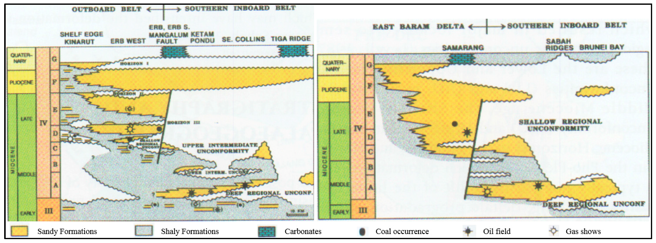
The X Field, which lies to northwest of the Southern Inboard Deformation Belt, is located in the outer shelf of the West Sabah Basin. Figure 1 shows the simplified geological map of Sabah outlining the Neogene Basins and their sub-basins. The Sabah Basin is a structurally complex basin with 12 km thick Neogene sediments deposited within the deep marine and progradational shelf-slope environment [1]. Figure 2 schematically shows the stratigraphy of several east–west tracts of the Sabah Basin. The sedimentary sequences of Sabah Basin are informally called “Stages”. The recognition of major unconformity-bounded sedimentary packages of Stages IVA (sedimentary sequence Stage IVA) to IVF (sedimentary sequence Stage IVF) resulted from its complex syn-tectonic sedimentary history [2,3]. Oil and gas exploration activities have been sparse in the Northeast Sabah Basin (Figure 1), where minor discoveries were found in deltaic sandstones. Other targets within the basin include deep water fans and carbonate build-ups. Adequate knowledge on facies distribution and depositional environment is essential to delineate hydrocarbon potential. Facies analysis is able to provide some predictability to the facies distribution of the area of interest or between the data points (wells). A facies model is ideal for summarizing the sequence of facies within a specific depositional environment [4]. Genetic description is advantageous, as it potentially adds some predictability to the analysis from the determination of the sedimentological controls over the geometry of facies and genetic associations with other facies. The interpretative description of facies may reflect a particular depositional process or depositional environment of a certain unit of strata.
Seismic and well log data are widely used for subsurface mapping, as they complement each other. Seismic data essentially provides information on the lateral extension and distribution of geological elements compared to wells or cores. They measure larger lateral areas between wells but with a limited vertical resolution compared to well data [6]. They are useful in depicting the regional setting on a larger scale. Well logs yield a finer vertical resolution of the geology at the well locations. A well log is a chart that shows a concise and detailed plot of the formation parameters versus depth. Different lithologies, porosity of rocks, as well as the pay zones can be identified through the interpretation of logs.
Various classification algorithms have been adopted for facies classification, such as generalized boosted regression model (GBM) [7], kernel support vector machines [8], partitioning algorithms [9], and neural networks [10,11]. These classification algorithms predict the discrete and continuous probability distribution of facies. The interpretation of different log data such as neutron porosity, shale volume, and water saturation was considered for lithofacies classification in these studies [7,8].
In this study, 3D seismic data will be used to characterize the stratigraphy and architecture of the depositional elements and infer the processes of deposition where appropriate. Representative and successive horizons will be selected and picked through the 3D seismic data. The horizons bear imprints of the geomorphological evolution of the area of interest. The well log interpretation includes gamma ray, neutron porosity, and water saturation, as a function of depth. Facies classification is a challenging task. It is significant for formation evaluation analysis and reservoir characterization. Its purpose is to distinctly define subsurface geology and build a better understanding of the depositional environment in the area. A facies model can be used for the construction of the depositional environment of the study area.
The proposed methodology will incorporate seismic information using a suitable range of seismic facies analysis techniques. The methodology should later be calibrated with seismic attributes for enhancement. Seismic attributes are used to assist interpretation at different scales, ranging from analyzing depositional systems to mapping detailed structures, stratigraphy, and rock properties. They enhance information that might be more subtle in the original seismic image to provide a better geological or geophysical interpretation. Depending on their geologic application, attributes are classified and categorized into three groups: (1) structural mapping and geomorphological identification, (2) resolution of thin beds and improving interpretability, and (3) porefill and lithology discrimination [12].
2. Materials and Methods
The identification of the lithofacies is achieved by integrating well log and 3D seismic data. Well log analysis is carried out based on the geophysical logs from four different wells including gamma ray, resistivity, and sonic logs. Gamma ray and resistivity logs are useful for the identification of lithofacies and hydrocarbon-bearing zones. Gamma ray facies trends generally reflect changes in the proportion of sandstone to shale, which in turn are inferred to record changes in the depositional energy of high to low current flow. The logs are also used for well correlation and seismic-to-well tie. The classification of lithofacies requires the estimation of the lateral distribution of each lithofacies with relative confidence at the cored wells as well as the estimation of the lithofacies at the non-cored wells.
Seismic interpretation generally assumes that coherent events observed on the seismic sections are reflections from acoustic impedance contrasts. These contrasts are associated with features that represent different geological structures [13]. Regions of differing seismic facies are delineated using descriptive terms that reflect large-scale seismic patterns, including reflection amplitude, continuity, and internal configuration of reflectors that is bounded by stratigraphic horizons. 3D seismic data could be useful in constructing images of depositional facies. In this study, the principle is to calibrate seismic response with geologic information at the well in order to extend prediction of the geology away from well locations. Figure 3 shows the workflow for optimizing the analysis.
Once the lithofacies are identified through well log and seismic data analysis, Sequential Indicator Simulation (SIS) is adopted in this study to map the distribution of facies in the study area. SIS is a pixel-based simulation method used for stochastic modeling of nonparametric properties, such as rock types. The continuous variable is transformed into a number of indicator variables and these indicator variables will be spatially modeled using variogram or covariance functions [14]. Indicator variograms characterize the spatial variations. SIS takes into account the spatial variation of observed data at the sampled locations and estimated variation at unsampled locations to create a facies model. Its conceptual simplicity and straightforwardness made the sequential algorithm one of the most widespread in geostatistical applications [15]. Although legitimate criticisms arise against SIS, such as the models appear unstructured and the indicator variograms only control two-point statistical measures, there are some good reasons to consider the technique [16]. The robust algorithm provides a straightforward way to transfer uncertainty in categories through to the resulting numerical models and the required parameters are easy to infer from inadequate data. SIS has also been widely studied and adopted in many other studies [14,16,17].
3. Results
Well data including logs, cores, and thin sections are often used to relate rock parameters with seismic data. In this study, only geophysical logs from wells M1, P1, U1, and S1 are used due to the lack of other well data. Taking wells M1 and S1 as examples, Figure 4 depicts the discrete lithofacies distribution (sand, shaly sand, and shale). The well log interpretation includes gamma ray, porosity, density, and water saturation, as a function of depth. Within the reservoir interval (1100 m to 1600 m), the amount of shale is low in well M1, whereas sandstone is high, and the amount of shale increases from well M1 towards well S1 as the amount of sandstone reduces. The shaly sequences were deposited as interlayers with sand bodies. The predicted percentage of the sand and shale/shaly sand distribution is 55.37% and 44.63%, respectively.
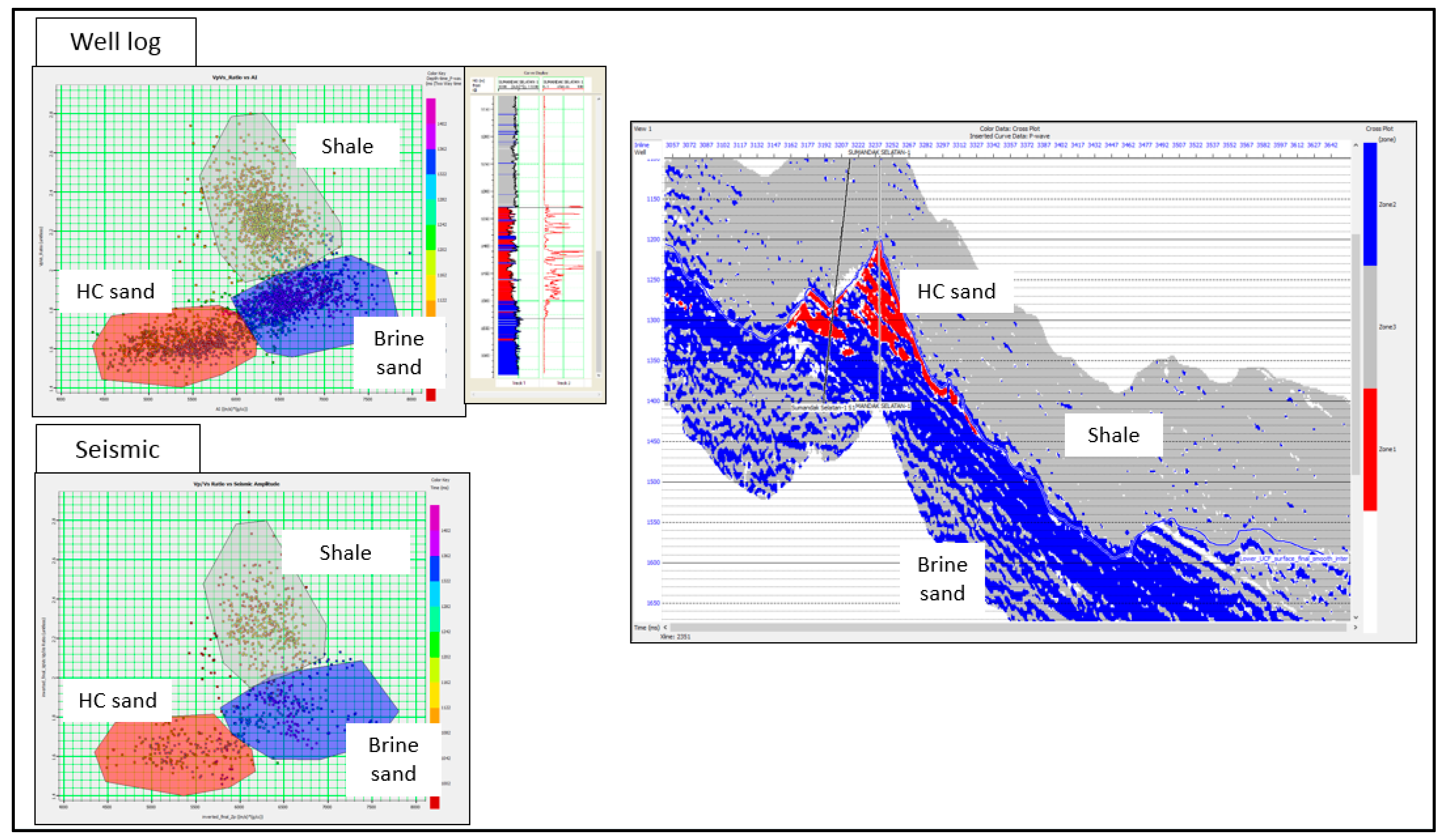
At well locations, cross-plot analysis of different parameters aids in the detection of zones with different lithologies. For example, Figure 5 indicates the scatter points of shale, HC (hydrocarbon) sand, and brine sand of the reservoir interval based on the cross plot of acoustic impedance (AI) versus Vp/Vs ratio (Vp and Vs are velocities of primary wave and secondary wave, respectively; i.e., the compressional velocity and shear velocity). AI-Vp/Vs cross-plot can be useful for hydrocarbon detection. Vp/Vs parameter on inversion results can be used to distinguish different types of lithofacies.
According to the interpreted seismic section and geological setting of the area, two prominent facies are identified, namely sandstone and shale due to their distinct lithological variations. Figure 6 shows the seismic section through Well S1 and the reservoir interval. Above the Shallow Regional Unconformity (SRU) are shale beds acting as reservoir seal. Shale is consistently found in all of the wells in X Field. Below the shale, high-amplitude reflections at the sandstone layer show the interface response of the hydrocarbon accumulations. The reflection within this interval has good continuity and high to moderate amplitude variation. The logs (gamma ray and porosity) show that at Well S1, the dominant lithofacies in the reservoir interval is sandstone. Referring to the stratigraphic scheme of Sabah Basin, the sequence above SRU is identified as Upper Miocene in age and categorized into Stage IVC.
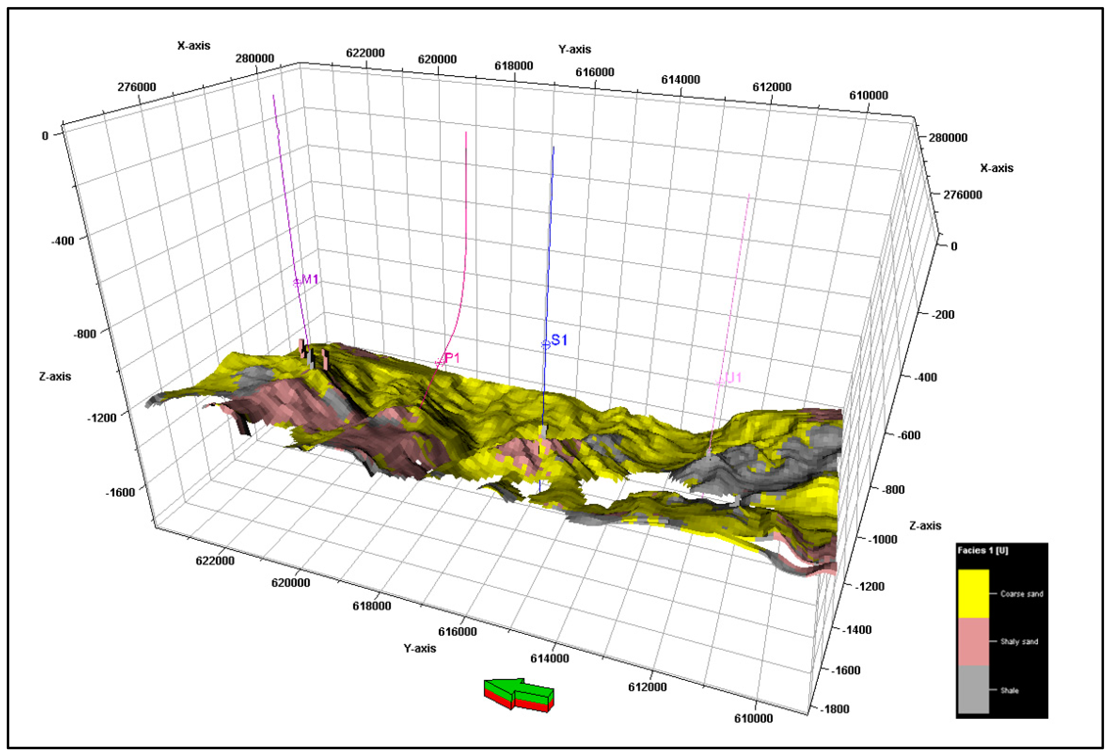
Using Sequential Indicator Simulation (SIS), a facies model is produced by the mean of distributing discrete facies throughout the model grid. In this study, two fundamental facies types were determined in the X Field reservoir based on the well data input and the spatial distribution induced by trend models. Figure 7 shows the facies model indicating the sand and shale distribution in the study area. Previous studies indicated that the area of interest is characterized by the East Baram Delta depositional environment (which includes deltaic, shelf, and slope sediments deposited in an overall progradational system from Middle Miocene to younger stages of Stage IVC (sedimentary sequence stage IVC) [18].
4. Conclusions
This study demonstrates an integrated approach using 3D seismic data and well logs to illustrate the distribution of facies in the X Field of Sabah Basin. From the well logs and seismic analysis, two prominent lithofacies were identified, namely sandstone and shale. The hydrocarbon bearing zone occurs below the shaly sequence, which acts as reservoir seal. The sandstone interval that contains the hydrocarbon bearing formation is bounded by the Shallow Regional Unconformity. The prominent facies identified in the study area were used as input for a facies distribution model. Integration of the seismic data analysis with wells information was able to refine the existing understanding on lateral and vertical facies distribution in the study area. The resultant facies map depicts the facies distribution in X Field. In order to obtain a better classification of lithofacies in the field, future work will focus on seismic attribute analysis and artificial neural network (ANN) technique. The analysis can take the form of seismic attribute extraction and classification of seismic facies based on the defined training data. The process aids in the evaluation of seismic features and will be a geomorphological approach to seismic interpretation.
Acknowledgments
The authors thank UTP for funding this research work and PETRONAS for providing the data.
Author Contributions
Jia Qi Ngui implemented the lithofacies classification workflow on seismic and well data; Maman Hermana contributed to log analysis, Deva Prasad Ghosh contributed to seismic analysis and Wan Ismail Wan Yusoff contributed to facies identification.
Conflicts of Interest
The authors declare no conflict of interest.
References
- Dennis, N.K.T.; Lamy, J.M. Tectonic evolution of the NW Sabah continental margin since the Late Eocene. GSM Bull. 1990, 27, 241–260. [Google Scholar]
- Mazlan, M.; MAroN, H.J. Basin types, tectono-stratigraphic provinces, and structural styles. In The Petroleum Geology and Resources of Malaysia; Petronas: Kuala Lumpur, Malaysia, 1999; pp. 79–111. [Google Scholar]
- Mazlan, M.; Leong, K.M.; Anuar, A. Sabah basin. In The Petroleum Geology and Resources of Malaysia; Petronas: Kuala Lumpur, Malaysia, 1999; pp. 501–542. [Google Scholar]
- Maliva, R.G. Facies analysis and sequence stratigraphy. In Aquifer Characterization Techniques, 1st ed.; Springer International Publishing: Cham, Switzerland, 2016; pp. 25–48. [Google Scholar]
- Leong, K.M. Geological setting of Sabah. In The Petroleum Geology and Resources of Malaysia; Petronas: Kuala Lumpur, Malaysia, 1999; pp. 475–497. [Google Scholar]
- Deep-reading technologies. Available online: https://www.geoexpro.com/articles/2009/06/deep-reading-technologies (accessed on 16 February 2017).
- Al-Mudhafar, W. Integrating well log interpretations for lithofacies classification and permeability modeling through advanced machine learning algorithms. J. Petrol. Explor. Prod. Technol. 2017, 7, 1023–1033. [Google Scholar] [CrossRef]
- Al-Mudhafar, W. Integrating kernel support vector machines for efficient rock facies classification in the main pay of Zubair formation in South Rumaila oil field, Iraq. Model. Earth Syst. Environ. 2017, 3, 12. [Google Scholar] [CrossRef]
- McCreery, E.; Al-Mudhafar, W. Geostatistical classification of lithology using partitioning algorithms on well log data—A case study in Forest Hill oil field, East Texas Basin. In Proceedings of the 79th EAGE Conference and Exhibition, Paris, France, 12–15 June 2017. [Google Scholar]
- Avseth, P.; Mukerji, T. Seismic lithofacies classfication from well logs using statistical rock physics. Petrophysics 2002, 43, 70–81. [Google Scholar]
- Tang, H.; Meddaugh, W.; Toomey, N. Using an artificial neural network method to predict carbonate well log facies successfully. SPE Reserv. Eval. Eng. 2011, 14, 35–44. [Google Scholar] [CrossRef]
- Ghosh, D.; Sajid, M.; Ibrahim, N.; Viratno, B. Seismic attributes add a new dimension to prospect evaluation and geomorphology offshore Malaysia. Lead. Edge 2014, 33, 526–545. [Google Scholar] [CrossRef]
- Sheriff, R.E.; Geldart, L.P. Exploration Seismology, 2nd ed.; Cambridge University Press: Cambridge, UK, 1982; pp. 349–420. [Google Scholar]
- Al-Mudhafar, W. Geostatiscal lithofacies modeling of the upper sandstone member/Zubair formation in south Rumaila oil field, Iraq. Arab. J. Geosci. 2017, 10, 153. [Google Scholar] [CrossRef]
- Emery, X. Properties and limitations of sequential indicator simulation. Stoch. Environ. Res. Risk Assess. 2004, 18, 414–424. [Google Scholar] [CrossRef]
- Deutsch, C. A sequential simulation program for categorical variables with point and block data: BlockSIS. Comput. Geosci. 2006, 32, 1669–1681. [Google Scholar] [CrossRef]
- Seifert, D.; Jensen, J.L. Using sequential indicator simulation as a tool in reservoir description: Issues and uncertainties. Math. Geol. 1999, 31, 527–550. [Google Scholar] [CrossRef]
- Stump, T.E. Review of the existing and future potential of the Sabah basin, offshore Malaysia. Unpublished work. 2004. [Google Scholar]
Figure 1.
Simplified geological map of Sabah outlining the Neogene basins, including the study area [5].
Figure 1.
Simplified geological map of Sabah outlining the Neogene basins, including the study area [5].

Figure 2.
Schematic illustration of the stratigraphy of Sabah Basin [3].
Figure 2.
Schematic illustration of the stratigraphy of Sabah Basin [3].

Figure 3.
Workflow for lithofacies identification using seismic and well log data.
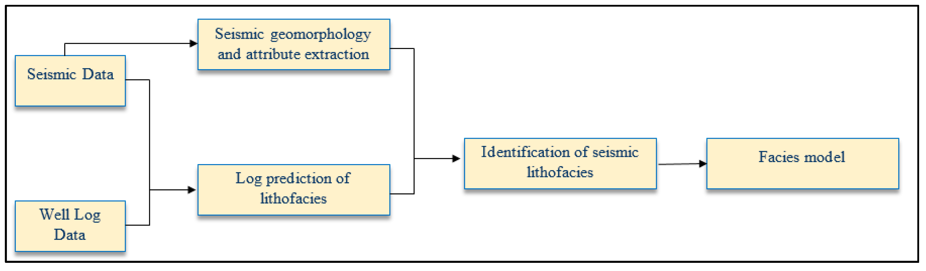
Figure 4.
(a) Base map of the study area showing the well locations. (b) Identification of lithofacies from Well M1 and Well S1. The gamma ray response distinguishes the low gamma ray value of sand from the higher value of shale.
Figure 4.
(a) Base map of the study area showing the well locations. (b) Identification of lithofacies from Well M1 and Well S1. The gamma ray response distinguishes the low gamma ray value of sand from the higher value of shale.
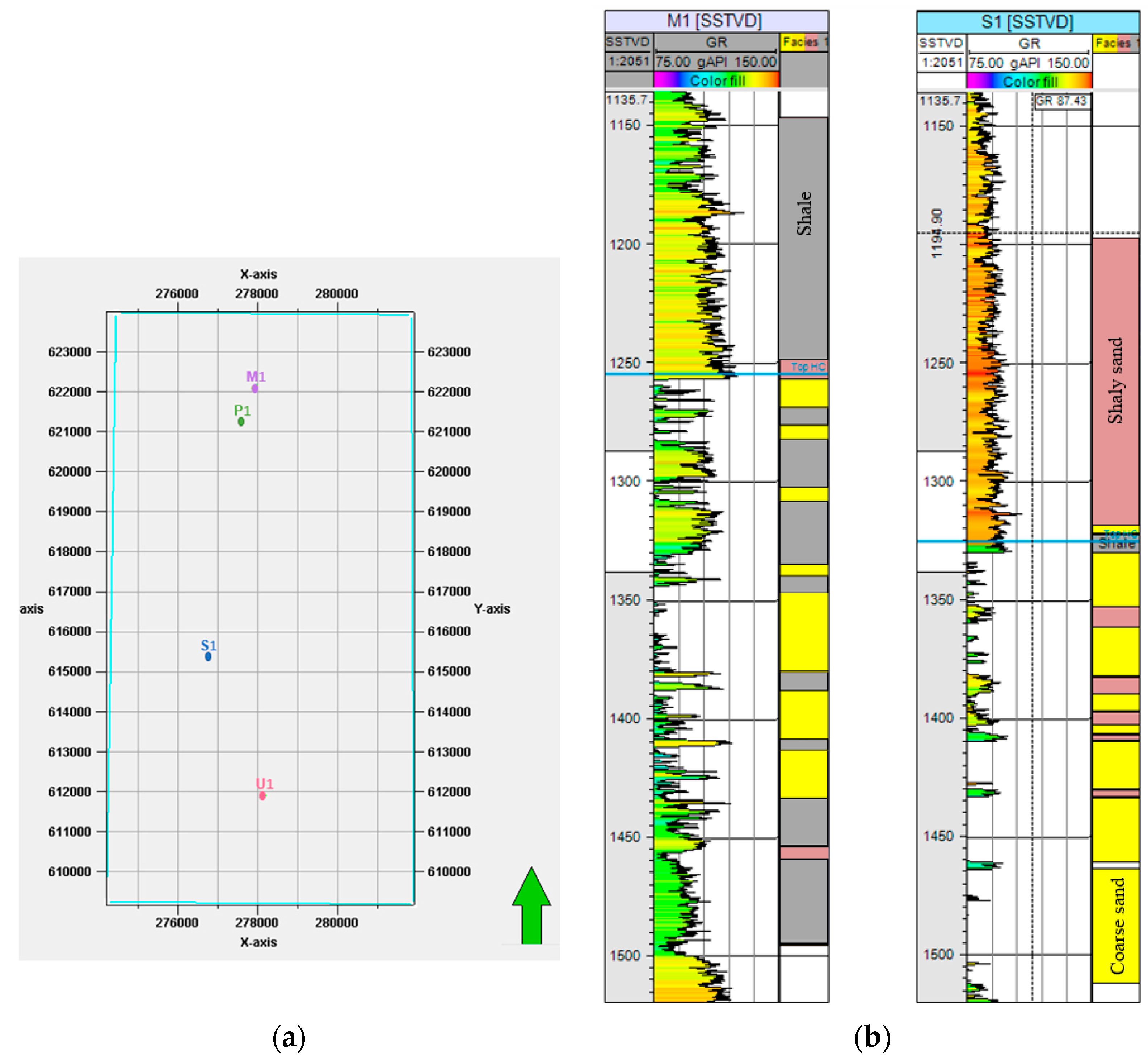
Figure 5.
AI-Vp/Vs cross-plot (left) and 3D seismic section (right) showing the separation of shale, HC (hydrocarbon) sand, and brine sand zones.
Figure 5.
AI-Vp/Vs cross-plot (left) and 3D seismic section (right) showing the separation of shale, HC (hydrocarbon) sand, and brine sand zones.

Figure 6.
Seismic section extracted from seismic volume in the position of Well S1.
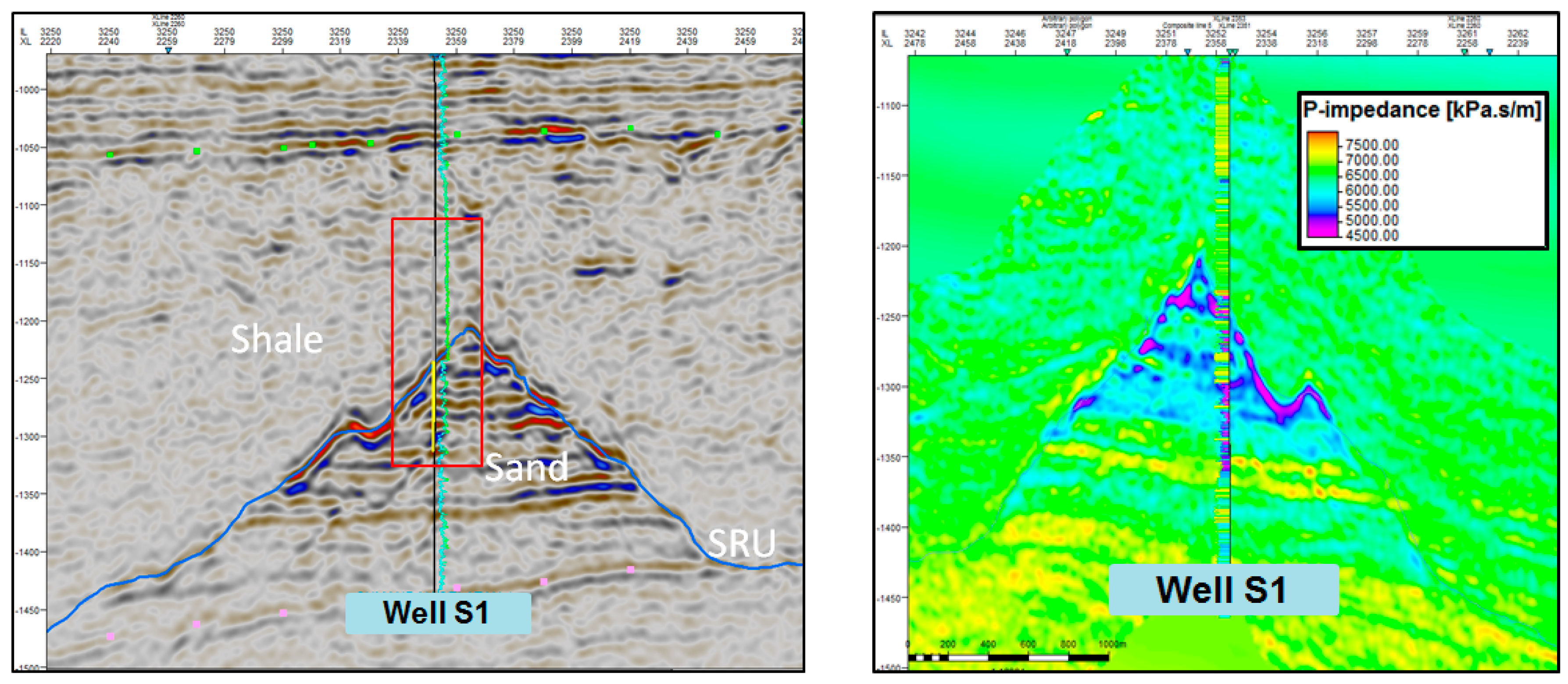
Figure 7.
Facies model indicating the distribution of the prominent facies (sand, shaly sand, and shale) in X Field. The upper layer is the top HC horizon (Shallow Regional Unconformity) and the base is the lower HC horizon (Upper Intermediate Unconformity). The number of grid cells is 78 in the I-direction and 149 in the J-direction, divided into 10 layers. The final geostatistical model has 113,960 total gridblocks for all the layers.
© 2018 by the authors. Licensee MDPI, Basel, Switzerland. This article is an open access article distributed under the terms and conditions of the Creative Commons Attribution (CC BY) license (http://creativecommons.org/licenses/by/4.0/).
Share and Cite
MDPI and ACS Style
Ngui, J.Q.; Hermana, M.; Ghosh, D.; Wan Yusof, W.I. Integrated Study of Lithofacies Identification—A Case Study in X Field, Sabah, Malaysia. Geosciences 2018, 8, 75. https://doi.org/10.3390/geosciences8020075
AMA Style
Ngui JQ, Hermana M, Ghosh D, Wan Yusof WI. Integrated Study of Lithofacies Identification—A Case Study in X Field, Sabah, Malaysia. Geosciences. 2018; 8(2):75. https://doi.org/10.3390/geosciences8020075
Chicago/Turabian StyleNgui, Jia Qi, Maman Hermana, Deva Ghosh, and Wan Ismail Wan Yusof. 2018. "Integrated Study of Lithofacies Identification—A Case Study in X Field, Sabah, Malaysia" Geosciences 8, no. 2: 75. https://doi.org/10.3390/geosciences8020075
Note that from the first issue of 2016, this journal uses article numbers instead of page numbers. See further details here.