Simulations of Moisture Gradients in Wood Subjected to Changes in Relative Humidity and Temperature Due to Climate Change

Abstract

Climate change is a growing threat to cultural heritage buildings and objects. Objects housed in historic buildings are at risk because the indoor environments in these buildings are difficult to control and often influenced by the outdoor climate. Hygroscopic materials, such as wood, will gain and release moisture during changes in relative humidity and temperature. These changes cause swelling and shrinkage, which may result in permanent damage. To increase the knowledge of climate-induced damage to heritage objects, it is essential to monitor moisture transport in wood. Simulation models need to be developed and improved to predict the influence of climate change. In a previous work, relative humidity and temperature was monitored at different depths inside wooden samples subjected to fluctuating climate over time. In this article, two methods, the hygrothermal building simulation software WUFI^® Pro and the Simplified model, were compared in relation to the measured data. The conclusion was that both methods can simulate moisture diffusion and transport in wooden object with a sufficient accuracy. Using the two methods for predicted climate change data show that the mean RH inside wood is rather constant, but the RH minimum and maximum vary with the predicted scenario and the type of building used for the simulation.

1. Introduction

The growing threat of climate change to cultural heritage has gained increasing awareness. The knowledge is due to findings from research projects which aim to predict future climate change and its impact on cultural heritage buildings and the indoor environment in those buildings. The Global Climate Change Impact on Built Heritage and Cultural Landscapes; Noah’s Ark Project (2004–2007) brought forward the fact that little attention had been paid to the impact of global climate change on cultural heritage and that this needed to be better recognised and perceived as relevant. Due to climate change, a range of direct and indirect effects were expected to be observed on built heritage [1,2]. The EU research project Climate for Culture: Damage Risk Assessment, Economic Impact and Mitigation Strategies for Sustainable Preservation of Cultural Heritage in Times of Climate Change (2009–2014) studied the impact and mitigation strategies for preservation of cultural heritage in times of climate change. The project developed simulation models to estimate the impact of future global climate change on the indoor environments in different types of buildings in different regions of Europe. According to the project, the indoor temperature (T) in non-heated buildings in parts of northern Europe will at first (2021 to 2050) increase, but in the far future (2071 to 2100) decrease [3]. Important research projects on improving energy efficiency of historic built heritage include, for instance, Sustainable Energy Communities in Historic Urban Areas (SECHURBA) (2008–2011) [4], and Energy Efficiency for EU Historic Districts’ Sustainability (EFFESUS) (2012–2016) [5].

So far, the main focus on energy efficiency measures of these projects has been on the buildings and the indoor environment and less on the effect on the objects housed in them. Historic buildings, such as churches, often have large interior volumes and a high air infiltration rate, which obstructs efforts to regulate indoor relative humidity (RH) and T. The buildings themselves are often of high cultural heritage value. Therefore, interventions, such as installation of air conditioning plants or alterations to the building envelope to decrease the air infiltration, are often restricted. Consequently, the interiors may be subjected to large daily, as well as seasonal, changes in both RH and T, much larger than the recommended climate criteria for hygroscopic museum objects [6]. For these reasons, it is important to also include hygrothermal monitoring and monitoring of mechanical deformation of heritage objects located in historic buildings. Moreover, it is central to find reliable modelling methods to be able to predict potential future impact of climate change. This was recognised by the Netherlands Organisation for Scientific Research (NWO) and Rijksmuseum Amsterdam in their report, The Conservation of Panel Paintings and Related Objects: Research agenda 2014–2020. It emphasised that a balance between preservation of art, energy cost and effects on buildings in the widest sense should be encouraged. It further suggests research topics which should comprise: modelling behaviour patterns including validation studies, experimental population studies, hygro-mechanical properties of ageing wood in panels and inter-laminar stress and fracture mechanics, which also affect paint layers [7].

Hygroscopic organic materials, such as wood, are particularly susceptive to changes in the ambient climate. With an increase in RH, wood will adsorb moisture from the ambient air and swell. With a decrease in RH, it will desorb moisture and shrink. If the changes in RH and T are significant, or frequent enough, permanent deformation or damage may occur. The moisture content (MC) in wood is defined as the mass of water in relation to the oven-dried wood, expressed as a percentage. Maximum swelling or shrinkage at certain RH may occur when equilibrium moisture content (EMC) is reached. It is defined as the MC at which the wood is neither adsorbing nor desorbing moisture from the ambient air. However, equilibrium will only follow if RH and T are constant for a long enough period of time for the wood to be fully acclimatised to the ambient air throughout. This may take a very long time and during real-life conditions it is uncertain if EMC is ever reached [8]. In a fluctuating climate, constantly moving moisture gradients will develop from the surface and inwards. Methods which can accurately monitor moisture movement in wood due to different RH and T combinations are few. Nevertheless, the study of moisture diffusion in wood is an important first step since it will contribute to an increased understanding of how deformation of wood and, thereby, also damage, or lack of damage, develop [9]. Various types of long-term wood electrical resistance sensors to monitor MC to predict the service life of wooden constructions have been tested [10,11,12,13]. However, some resistance methods have shown to be connected with measuring errors. Because wood shrinks and swells, the contact between the wood and the resistance pins may vary, resulting in inaccurate readings [11]. The volume of the wooden sample and the distance of sensor to the surface do also affect the measuring results [14]. Therefore, a method to monitor RH and T distribution in wooden samples was instead developed, and is described in [15]. The monitored data can also easily be converted to MC according to Equation (2) of this article. The method is based on small RH and T sensors, which are inserted into drilled holes in wooden samples. The sensors are located at different depths in order to monitor the moisture movement inside the wood. The samples were exposed to step-changes and fluctuations in RH and T in a climate chamber. The advantage is that the method can be used in in situ monitoring campaigns in historic buildings [16]. These data can be further used for simulation modelling to predict, for instance the future effects of climate change on wooden objects. To measure RH and T inside the material instead of using the general room climate data reduces the risk of misinterpretation since local microclimates found in historic buildings, for instance behind paintings hanging on walls or inside closed cabinets, are also influencing the objects.

To study the effect of climate change on heritage objects housed indoors, it is important to take the building type into account, because their response to the outdoor climate will influence the indoor climate. Climate change induces variations in both long- and short-term behaviour of the climate system, resulting in warmer weather with stronger and more frequent extreme conditions [17]. Such variations can affect the hygrothermal performance of building components on different time scales [18,19]. Hence, the actual effect on the objects is the combination of the outdoor climate and the kind of building.

In the first part of this article, the aim was to further develop and compare simulation methods which can study the hygrothermal effect on wooden objects during variations in RH and T. It is based on existing data from previously performed laboratory experiments [16]. Two simulation methods were chosen: WUFI^® Pro software and a simplified analysis method (Simplified model). In the second part, the aim was to simulate the effect of predicted climate change scenarios to wooden objects in different types of buildings. This was done by using two different methods. Firstly, a verified method used for the impact assessment of climate change, which is based on synthesizing three sets of 1-year weather data sets, representing typical, extreme-cold and extreme-warm conditions [20,21]. The method helps to run faster simulations while climate uncertainties and extreme conditions are taken into account. The synthesized representative weather data sets were then applied to two different types of generic buildings, i.e., a typical heavy and a typical light constructed house. Secondly, within the Climate for Culture project, simulated climate data due to climate change has also been produced [22,23]. These data were used by the Fraunhofer Institute for building physics in order to generate data of the indoor climate for certain case studies all over Europe. To show the simulated effect of future climate change on the indoor climate an existing building, Roggersdorf church in Bavaria, Germany, was also used in this study. It is a small heavyweight building without any strategy for climate control. The generated climate data was finally used to study the simulated effect on the moisture distribution in wood assumed housed in the generic and existing buildings according to the WUFI^® Pro model.

The principal conclusions are that both WUFI^® software program and the Simplified methods are capable of quite accurate predictions of the moisture conditions inside wood at temperature and RH variations of 7–25 °C to 35–75%. Likewise, the two methods are generally in agreement, while the influence on wood is generated from simulated climate change data. The mean values are rather constant during the simulated periods. However, different types of climate predictions from different kinds of buildings generate variances in minimum and maximum RH inside wood.

2. Materials and Methods

2.1. Experimental Data

In a previous work by Bylund Melin et al., a method was developed and thoroughly presented to monitor moisture transfer over time. Tangential cut wood samples (Scots pine, Pinus sylvestris L.) were subjected to various changes in ambient climate in a laboratory climate chamber. The aim of this work was to study the impact of the effect of fluctuating RH and T which can be found in less climate-controlled historic buildings [15]. In this study, Scots pine was chosen, since it is a wood species common in cultural heritage objects in Sweden. The method is also designed to be used with other types of wood. The dimensions of the wood samples used in the experiments were 200 mm × 45 mm × 45 mm. The monitoring device consists of small RH and T sensors (MSR loggers), which were inserted from the reverse side of the wooden samples down to different depths (1, 4 and 7 mm from the front side). Due to the monitoring at several depths, it is possible to study in detail the effects of changing RH or T as well as the combined effect of changing RH and T. The method can be used in controlled laboratory settings as well as in situ locations, such as historic buildings. The chosen dataset used here was taken from [16]. It consists of 10-day long step-changes, in which the ambient RH in the ambient climate chamber varied between 35 and 75% RH. The measured data used during the period from day 40 to day 60 consists of two measuring periods, which were attached [16] (Figure 2). Less climate-controlled historic buildings can suffer from RH well above 75%, and heated buildings often show very low RH levels during winter and should have been included in the experiments. However, due to limitations of the climate chamber at low temperatures, the experiments were limited to the 35–75% range [16].

The monitored and simulated data used in this article are publicly available at Chalmers University of Technology: http://www.byggnadsteknologi.se/.

2.2. Simplified Theoretical Analysis

Several numerical simulation programs were analysed in the HAMSTAD project [24]. The project presented five numerical benchmark cases for the quality assessment of simulation models for one-dimensional heat, air and moisture (HAM-) transfer. Several solutions from different universities and institutes were compared. Consensus solutions could be found. However, the various presented calculation results varied somewhat. The Simplified model is based on a linearization of the sorption curve and constant water vapour diffusion. It does not need a specific software program; instead the calculations can be performed in a simple Excel spreadsheet. In [24], various types of numerical solutions are applied to handle the moisture transfer benchmark cases. These give a background to the complexity of the problem at hand and the expected acceptable accuracy.

The Simplified model is presented in this section. In this, hysteresis is neglected and the sorption isotherm is assumed to be linear. The moisture transfer is driven by the gradient in humidity by volume, v (kg/m³). The transport coefficient, ${\delta }_v^0$ (m²/s), is assumed to be constant, i.e., independent of moisture levels. The developed model allows for the development of handy analytical expressions which can give a lot of insights. In Section 4.1, it is also shown that the simplified analysis gives reasonable results in a comparison with experimental results.

The moisture balance equation assuming constant, but time dependent, temperature through the material becomes, with $\phi \left(x,t\right)$ (−) representing the relative humidity in the material:

$$\begin{array}{l}-\frac{\partial }{\partial x}\left(-{\delta }_v^0\frac{\partial v}{\partial x}\right)=\frac{\partial w}{\partial t}\\ \iff \\ {\delta }_v^0\frac{{\partial }^{2}v}{\partial x^2}={\delta }_v^0{v}_s(T)\frac{{\partial }^2\phi }{\partial x^2}=\frac{\partial w}{\partial t}=\frac{\partial w}{\partial \phi }\frac{\partial \phi }{\partial t}=\xi \frac{\partial \phi }{\partial t}\end{array}$$

(1)

Here, w(φ) (kg/m³) is the moisture content per volume unit, which depends on the relative humidity only since hysteresis is neglected in the simplified model. The relation $v=v_s\left(T\right)\cdot \phi$, where v_s represents the humidity by volume at saturation has been used. The following relation with the moisture content u(−) (sometimes referred to as the MC) can be used to translate between units:

$$u=\frac{w(\phi )}{{\rho }_{dry}}$$

(2)

The term in the denominator is the dry density of the wood (kg/m³).

As a part of the simplified model, the slope of the sorption curve is assumed to be constant:

$$\frac{\partial w}{\partial \phi }=\xi$$

(3)

Introducing the water vapour moisture diffusivity a_v (m²/s):

$$\frac{{\partial }^2\phi }{\partial x^2}=\frac{1}{a_v(t)}\frac{\partial \phi }{\partial t}{a}_v(t)=\frac{{\delta }_v^0{v}_s(T(t))}{\xi }$$

(4)

The next step is to analyse the more complicated case with simultaneous step-wise variations in RH and boundary temperature. The wood panel is exposed to the following varying load at x = 0 neglecting any surface resistances:

$$\{\begin{array}{l}{\phi }_i={\phi }_0+{\displaystyle \sum _{n=1}^N\left({\phi }_n-{\phi }_{n-1}\right)\cdot H\left(t-t_n\right)}\\ T_i=T_0+{\displaystyle \sum _{n=1}^N\left(T_n-T_{n-1}\right)\cdot H\left(t-t_n\right)}\end{array}t>0t_n>0$$

(5)

Here, H(t) represents the Heaviside unit-step function; it is equal to zero for times less than zero, and one for times greater than zero.

Before time t₁ the wood sample has been exposed to a stable climate (RH, temperature) of $\left({\phi }_0,T_0\right)$ for a very long time. The step at time t_n change the boundary value both for the relative humidity and the temperature by the amount $\left({\phi }_n-{\phi }_{n-1}\right)$ and $\left(T_n-T_{n-1}\right)$ respectively. Equation (4) needs to be solved with boundary condition (5).

Simplified Analysis—Step-Change, Periodic Variation and Time Varying Moisture Diffusivity

First some simple, but handy, analytical solutions for cases from [25] with constant temperature, $T=T_0$, and semi-infinite region will be presented.

With one step change at time zero at the wood surface at x = 0:

$${\phi }_i={\phi }_0+\Delta \phi \cdot H(t)t>0$$

(6)

The analytical solution [25] for a semi-infinite domain, with constant temperature, is:

$$\phi (x,t)={\phi }_0+\Delta \phi \cdot \mathrm{erfc}\left(\frac{x}{\sqrt{4a_v\cdot t}}\right)x\ge 0,t\ge 0$$

(7)

Here, erfc is the complimentary error function.

The penetration depth, i.e., the depth to which approximately half the disturbance of what happened at the boundary has propagated:

$$x_{0.5}=\sqrt{a_v\cdot t}$$

(8)

Typically, for wood, with ${\delta }_v^0$ = 0.5 × 10⁻⁶ m²/s and ξ = 120 kg/m³ at 21 °C [25], this depth is around 0.0005 m after 1 h, 0.0007 m after 2 h, 0.003 m after 1 day and 0.007 m after a week. These very limited penetration depths also mean that the assumption of semi-infinite region is not really a limitation. This assumption is valid if the real thickness of the material layer is on the order of 2–5 times the penetration depth.

The following variation at the wood surface at x = 0 is given:

$${\phi }_i={\phi }_0+{\phi }_A\cdot \sin (\frac{2\pi t}{t_p})$$

(9)

Here, t_p (s) is the time period of the sinusoidal variation. The analytical solution [25] becomes:

$$\phi (x,t)={\phi }_0+{\phi }_A\cdot e^{-x/d_{pv}}\sin (\frac{2\pi t}{t_p}-x/d_{pv})x\ge 0$$

(10)

The penetration depth $d_{pv}$ (m), i.e., the depth were the amplitude of the RH has diminished with a factor exp(−1), approx. 0.37 reads:

$$d_{pv}=\sqrt{\frac{a_v{t}_p}{\pi }}$$

(11)

Typically, for wood, with ${\delta }_v^0$ = 0.5 × 10⁻⁶ m²/s and ξ = 120 kg/m³ at 21 °C [25], this depth is around 0.001–0.002 m for a diurnal variation (t_p = 24 h) and 0.03 m for a yearly one.

The following variable substitution is introduced in order to solve (4) with time-dependent moisture diffusivity:

$$\tau (t)={\displaystyle \underset{0}{\overset{t}{\int }}{a}_v(t^{\prime })d{t}^{\prime }}$$

(12)

This changes (4) to:

$$\frac{{\partial }^2\phi }{\partial x^2}=\frac{\partial \phi }{\partial \tau }$$

(13)

This equation is similar to the classic one-dimensional heat conduction or diffusion equation with the diffusivity term equal to one. The equation is linear when using this transformed time variable; thus, superposition techniques can be used. Therefore, only the solution of a unit-step change is needed to handle the boundary conditions according to (5).

It is assumed that the penetration of moisture into the wood is much less than the thickness of the sample and that the initial relative humidity is ϕ₀. With a step in relative humidity of Δϕ, we then get:

$$\phi (x,\tau )={\phi }_0+\Delta \phi \cdot \mathrm{erfc}\left(\frac{x}{\sqrt{4\tau }}\right)x\ge 0,\tau \ge 0$$

(14)

The complete solution, referred to as the Simplified model, of (4) and (5) then becomes:

$$\phi (x,t)={\phi }_0+{\displaystyle \sum _{n=1}^N\left({\phi }_n-{\phi }_{n-1}\right)\cdot \mathrm{erfc}\left(\frac{x}{\sqrt{4\cdot \tau (t-t_n)}}\right)}$$

(15)

2.3. WUFI^® Pro Simulation Method

WUFI^® is a well-known method to calculate transient heat and moisture transport in building materials. It was created by Künzel, who developed a differential equation system based on the physical principles of heat and moisture transport for determining the moisture behaviour of multilayer building structures under natural climatic boundary conditions [26]. This was numerically implemented in the WUFI^® software program, further refined at the Fraunhofer Institute for Building Physics and verified with the assistance of the experimental field test site in Holzkirchen. The program WUFI^® Pro is suitable to simulate the temperature and moisture transport inside individual layers of composite materials. WUFI^® Pro was originally developed for the simulation of the hygrothermal behaviour of construction parts. The program was first used for the examination of the behaviour of artworks when exposed to climatic fluctuations by Holl. The simulations were validated by a dummy painting on canvas with determined material data, which was put with different distances on the inside of an exterior wall of a test building [27].

Since the WUFI^® material database does not include data for Scots pine, the simulations were instead carried out on Spruce (radial cut). However, in contrast with the Simplified model, the database includes data on the sorption isotherm as well as the water vapour diffusion resistance. The value for water vapour diffusion equivalent air layer thickness (sd-value) for the reverse side of the wooden samples was set at 1000 m, since the wooden samples were actually covered with aluminium foil on all but one side (the measuring front side). The initial RH was 77% and the initial T was 15.4 °C.

3. Impact of Future Climate Change on Wood

The Simplified model and WUFI^® Pro simulation method were also used to study the impact of predicted climate change on wooden objects housed in two different generic buildings located in Gothenburg, Sweden and an existing church (Roggersdorf church) in Bavaria, Germany. Two different hygrothermal simulation methods were used to predict the climate change and are presented below.

3.1. Hygrothermal Simulations of Future Climatic Conditions in Two Generic Buildings

Due to the existence of climate uncertainties and the need for considering several future climate scenarios, there will be large datasets to take into account, which makes the assessment time-consuming [28]. A method has been developed for creating representative weather data sets for future climatic conditions, considering typical and extreme conditions [20]. More than energy simulations, the proposed approach has been tested and verified for the hygrothermal simulation of building components by simulating the moisture conditions in the outer façade layer of a wooden frame wall in WUFI [21]. The approach was adopted in this work, which is based on synthesizing and using three sets of 1-year weather data, representing future climatic conditions for 2070–2099: (1) typical downscaled year (TDY), (2) extreme cold year (ECY), and (3) extreme warm year (EWY). The representative weather data were synthesized out of RCA4, the 4th generation of the Rossby Centre regional climate model (RCM) [29]. Considering Gothenburg and two Representative Concentration Pathways (RCPs) in this study, RCA4 downscaled three global climate models (GCMs) to the spatial resolution of 12.5 km²: CNRM-CM5 (for RCP4.5 and RCP8.5), ICHEC-EC-EARTH (for RCP4.5 and RCP8.5) and IPSL-CM5A-MR (for RCP8.5), resulting in five different climate scenarios. This means that the 1-year representative weather data sets (TDY, ECY and EWY) were synthesized considering 30 years of data for five different scenarios. More details on climate scenarios and calculating climate parameters are available in [20,30].

The three sets of 1-year weather data were applied on two types of generic buildings: (1) A non-habited light house (vapour concentration indoors equal to the outdoors and indoor T based on floating 24 h value of the outdoor T, plus 2 °C) and a heavy house (vapour concentration indoors equal to outdoors, plus 0.5 g/m³, indoor T based on floating one week value of the outdoor T plus 1 °C).

3.2. Hygrothermal Simulations of Future Climate Conditions in Roggerdorf Church

Within the Climate for Culture project, the Max Planck institute produced data sets for the recent past (1960–1990), the near future (2020–2050) and the far future (2070–2100) for the calculated future climate scenario A1B [31]. These three scenarios were applied to the Roggersdorf church by the Fraunhofer Institute for building physics in order to generate data of the indoor climate and the effect on wood.

4. Results

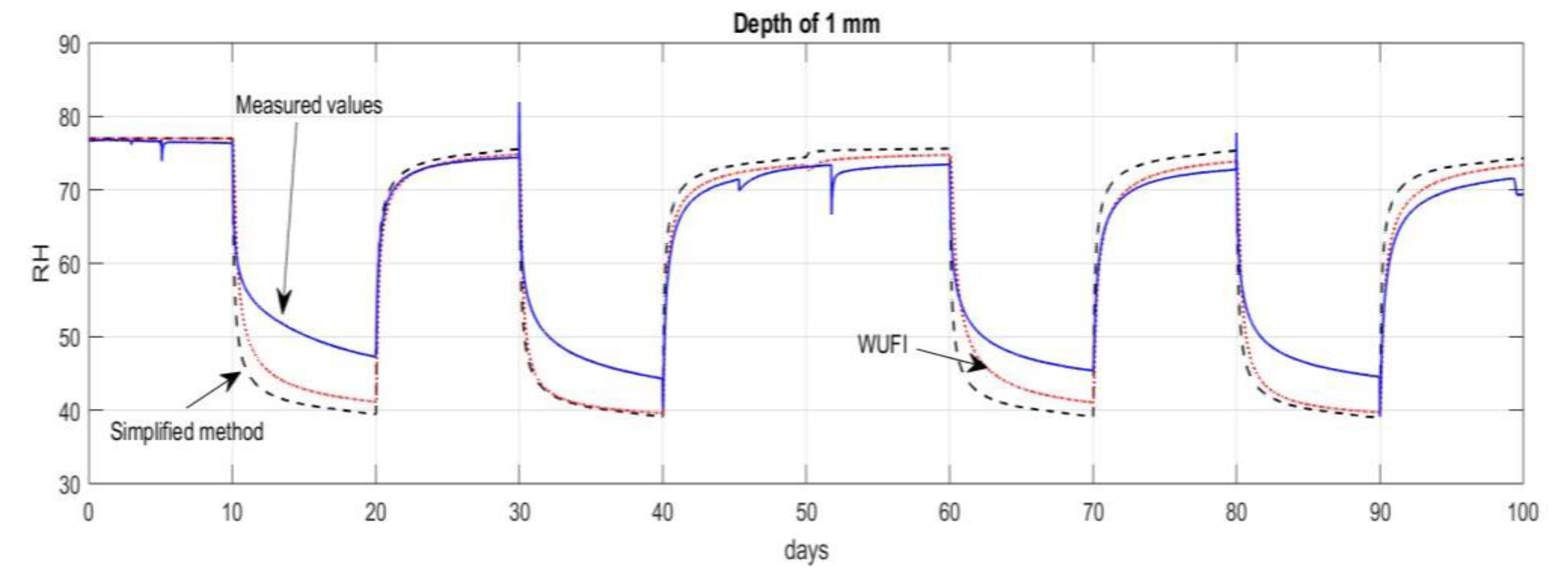
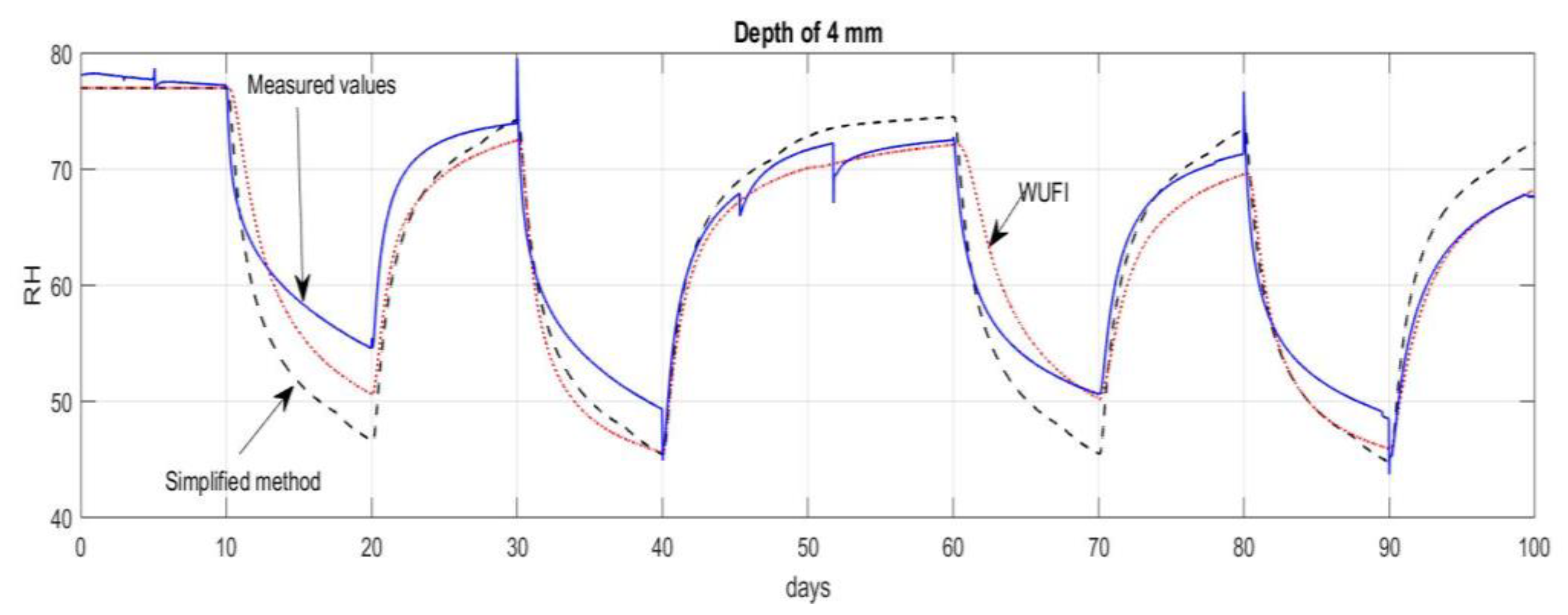
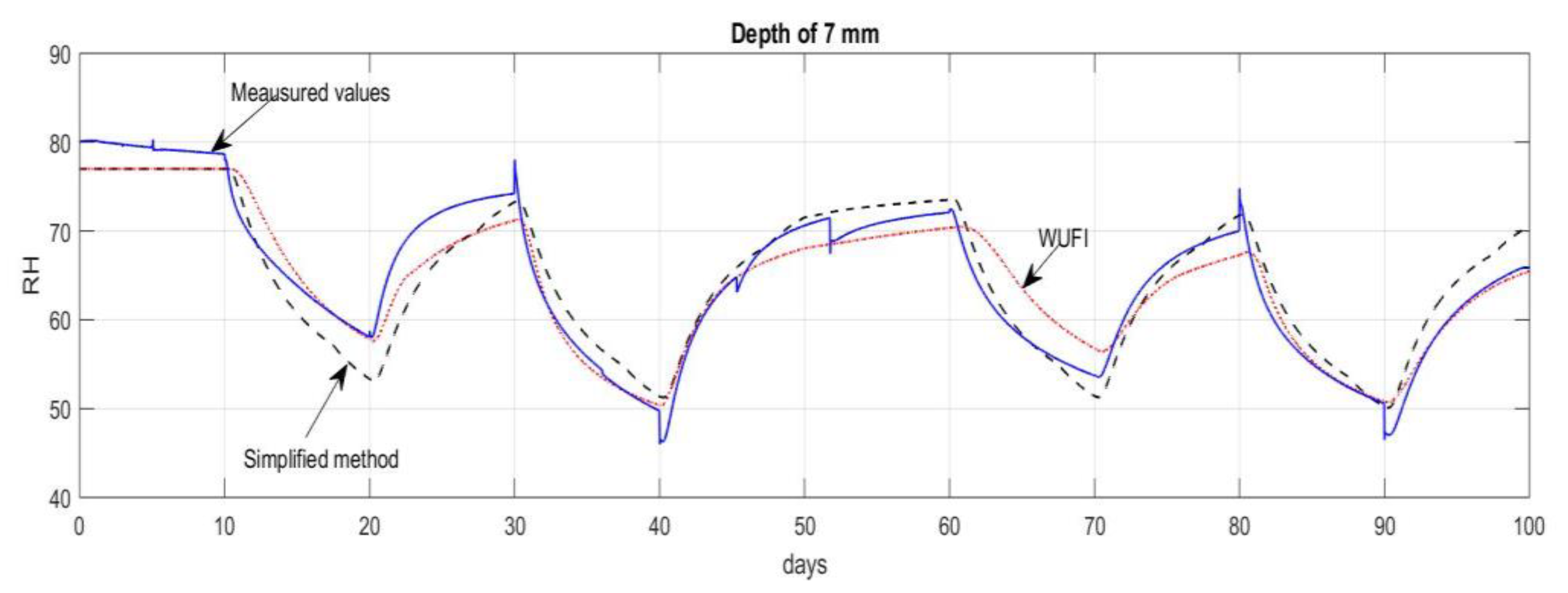
4.1. Comparison of the WUFI^® Pro and the Simplified Model

The measurements performed in [16] were used to validate the Simplified model and to compare it with WUFI^® Pro and the measured data. In these measurements the boundary RH and temperature vary in intervals of 10 days over a whole period of 100 days. In the Simplified model, this means that a_v basically varies every 10-day period. Thus, the variable $\tau \left(t\right)$ (12) is represented by a continuous curve built up by piece-wise linear segments, with the slope depending on a_v. The data used in the simulation was ${\delta }_v=0.5\times {10}^{-6}$ m²/s and ξ = 80 kg/m³.

The results for WUFI^® Pro and the Simplified model in relation to the measured data at the depth of 1, 4 and 7 mm can be seen in Figure 1, Figure 2 and Figure 3. According to the error analysis and comparison with the HAMSTAD benchmark, both simulation methods show generally excellent compliance with the measured data. At 1 mm depth (Figure 1), the two simulation methods overestimate the results on desorption, while on adsorption they are much closer to the measured values. The WUFI^® calculation method is generally closer to the measurements than the Simplified model. This tendency is not as clear at 4 and 7 mm depth. In fact, on 7 mm (Figure 3) the simulation on desorption is more conformed compared to the adsorption.

In summary,

Table 1. Average difference and standard deviation based on hourly values between measured and modelled result in the 100 days measured.

	The Simplified Model		WUFI® Pro Simulations
Depth (mm)	Average Difference (%)	Standard Deviation (%)	Average Difference (%)	Standard Deviation (%)
1 mm	1.6	4.9	1.6	3.4
4 mm	1.1	3.2	1.2	2.5
7 mm	0.1	2.9	0.3	2.5

shows the average difference and standard deviation between the two models and the measured data. The two methods are similar in their results, and both methods show a larger difference at 1 mm depth than at 7 mm depth.

Despite the reported average difference and rather small standard deviation (Table 1), the WUFI^® calculation method shows a generally closer agreement with the measured data compared to the Simplified model. The results are not in full agreement throughout, as can be seen in Figure 1, Figure 2 and Figure 3.

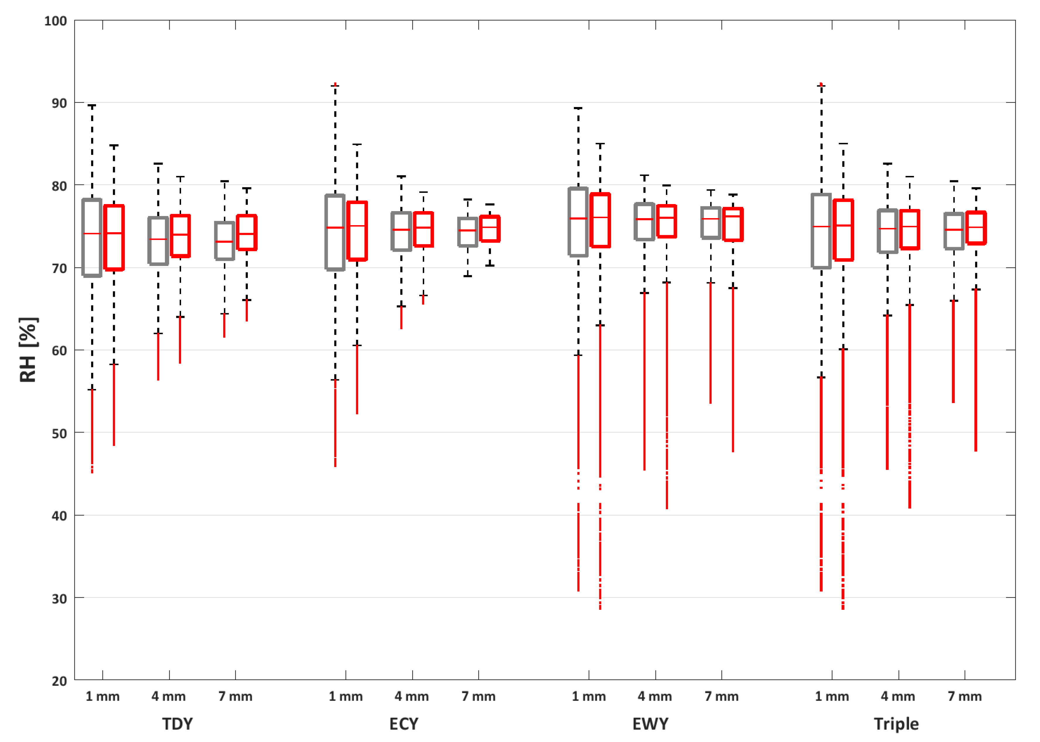
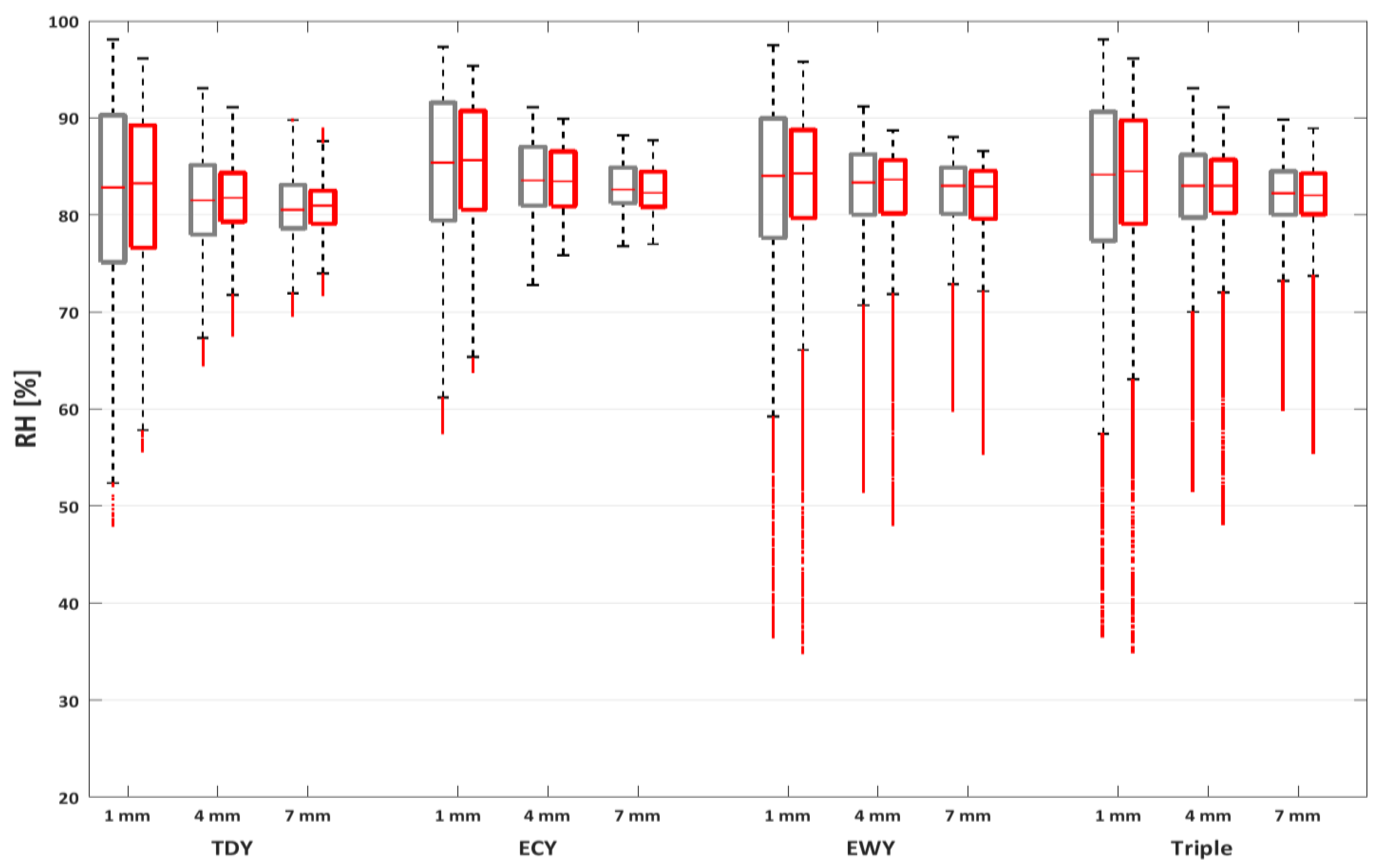
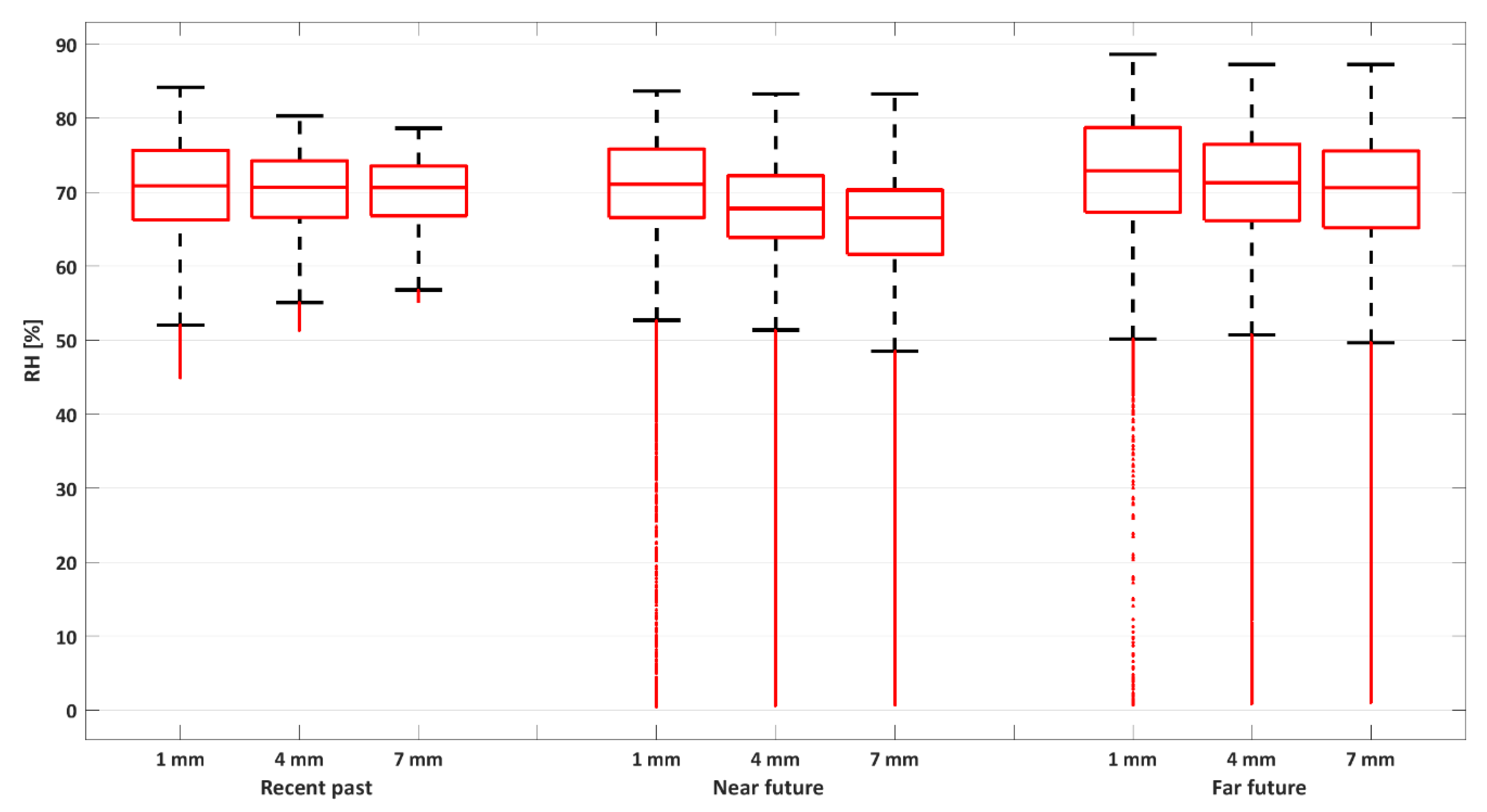
4.2. The Effect on Wood Using Hygrothermal Simulations of Future Climatic Conditions

The hygrothermal influence at 1, 4 and 7 mm depth in wood due to predicted climate change are presented in Figure 4, Figure 5 and Figure 6. For the Roggersdorf church, simulation only the WUFI^® Pro model was used.

Distributions of the calculated RH values inside the wood at different layers are shown for the light and heavy buildings respectively in box-and-whiskers plots in Figure 4 and Figure 5. Distributions are divided into four major groups; the first three (TDY, ECY and EWY) are based on the applied weather data (see Section 3.1) and the last one (Triple) contains all three groups. As has been shown previously [20,21], the distribution of typical and extreme conditions together is the most representative one.

Comparing the WUFI^® Pro method and the Simplified model shows that the mean values indicate close correlation. However, the Simplified model results in wider distributions of RH values, which is visible by having larger interquartile ranges (compare the size of boxes between two methods in the figures) and whiskers (outliers are almost in the same range for both methods, highly influenced by weather conditions). By getting deeper in the wood, differences between two methods decrease. For example, RH distributions among two methods are more similar in the depth of 7 mm than 1 mm.

For the generic buildings, it is clear that the mean RH in wood is lower in the light building type (approximately 73–77% RH at all depths) and higher in the heavy building type (approximately 80–85% RH at all depths). However, RH is generally more stable in the wood located in the heavy building, which is shown by the size of the larger boxes and the more bunched whiskers and outliers. An extreme cold year results in more stable RH inside the wood compared to an extreme warm year.

The data from Roggersdorf church (Figure 6) shows mean values of approximately 67–73% RH, slightly lower than the light building in Figure 4. RH is reduced in the near future, but increases in the far future. The distribution of RH inside wood is much larger (smaller boxes and more spread out whiskers) for Roggersdorf in relation to the two generic examples.

The predicted outdoor data from the two regions where the buildings are located are shown in

Table 2. Predicted yearly average outdoor T and RH in Gothenburg (affecting the generic buildings) and the 30 years average of Bavaria (affecting the Roggersdorf church).

	Gothenburg (One Year)			Bavaria (30 Years)
	Temperature (°C)	Relative Humidity (%)		Temperature (°C)	Relative Humidity (%)
TDY	9.109	82.98	Recent past	9.8	70.4
ECY	4.131	85.08	Near future	10.6	71.2
EWY	13.54	84.15	Far future	11.6	72.1

. It shows that RH is higher in Gothenburg, located on the west coast of Sweden in comparison with Bavaria, which is located inland. However, average RH is similar within each prediction situation (82.98–84.15% RH in Gothenburg and 70.4–72.1% RH in Bavaria). The temperature increases in Bavaria but does not reach the extreme warm weather predicted in Gothenburg. Due to the forecasted increase in T and RH for the far future scenario in Roggersdorf, T and RH inside the wooden samples in the Roggersdorf church increase as well (Figure 6). Due to the different time scales of the two prediction models, further comparison is difficult.

5. Discussion

To monitor moisture transport in wood (and other cultural heritage materials), it is essential to be able to validate and adjust simulation methods. This is the first effort known to the authors and it gave unexpectedly good results. It is believed that both methods can be used and developed further to estimate the impact of altered indoor environments to wooden objects in historic buildings subjected to changing heating regimes of the buildings or due to global warming. Although the WUFI^® Pro simulation performed slightly better, the Simplified model has an advantage in that it is easy to use and does not need specific software. It is assumed that for the simulation using a complex composite material such as a panel painting, WUFI^® will be more accurate, but this still has to be proven. The previously mentioned HAMSTAD project [24] presents a spread in results between different numerical methods. Even though the benchmark cases were not the same as the one in this paper, the performance of the Simplified method can very well match any of the other numerical ones, i.e., the difference between the Simplified model and WUFI^® Pro is in the parity of the difference between the different numerical solutions in [24]. The Simplified model presented assumes a semi-infinite flow domain. This may sound limiting but the method is applicable with good accuracy as long as the penetration depth is smaller or of the same magnitude as the exposed layer thickness. The penetration depth is on the order of millimetres, as shown in Section 2.2. The Simplified model can rather easily be extended to also cover the case with surface resistances.

To the best knowledge of the authors, this is the first time a simple analytical solution for the penetration of moisture in to wood during cycling of both temperature and RH is presented that can match a state-of-the-art numerical moisture transfer program such as WUFI^® Pro in accuracy. The model can rather easily be incorporated in a simple spreadsheet program such as Excel to calculate durability indicators.

Using the two methods to study the impact of climate change was tested within this work. Some of the results were expected, for instance that RH in the wood was higher during extreme cold weather conditions compared to extreme warm weather conditions. The larger difference between minimum and maximum RH inside the wood during summer could result in larger mechanical strain of wood and consequently permanent deformation. On the other hand, during extreme cold, the generally higher RH can result in increased risk for mould growth.

Interestingly, by getting deeper in the wood, differences in RH between the two methods decrease. This might be because of a difference in the boundary condition. In WUFI^® Pro, a water vapour surface resistance is considered, while this is omitted in the Simplified model. This difference is of minor importance deeper into the wood. Another explanation could be the depth of the drilled holes. Especially at 1 mm depth, there is a risk that the thickness is not exact, and this can make the results uncertain. It is possible that this is one reason there is a larger difference between the measures and simulated data at this depth compared to 7 mm. Therefore, the method used here should be validated further.

The use of spruce instead of Scots pine in the WUFI^® Pro hygrothermal simulation software poses an uncertainty in the simulation. To be more precise in the simulation, it is necessary to be as realistic as possible in the input data.

6. Conclusions

It has been shown that both methods, the Simplified model and the WUFI^® Pro hygrothermal simulation software, are able to simulate moisture diffusion and transport in wooden objects with sufficient accuracy. Using them to predict the effect of future climate change gave likely results, which further validate the methods. It gives a good indication of how wooden objects will react due to future climate change. Several future studies are possible while further developing the measuring method and refining the models. An example would be monitoring moisture transport in three-dimensional objects subjected to the environment from more than one side as well as painted wooden objects. To relate moisture transport to deformation (elastic and plastic) of wooden samples and real objects is also an important future task in order to better understand and assess climate-related damage processes to valuable cultural heritage artefacts.

References

1. Sabbioni, C. Noahs Ark Report Summary: Final Report Summary—Noahs Ark (Global Climate Change Impact on Built Heritage and Cultural Landscapes). 2011. Available online: https://cordis.europa.eu/result/rcn/47770_en.html (accessed on 8 April 2017).
2. Anthem Press. The Atlas of Climate Change Impact on European Cultural Heritage: Scientific Analysis and Management Strategies; Sabbioni, C., Brimblecombe, P., Cassar, M., Eds.; Anthem Press: London, UK, 2012. [Google Scholar]
3. Leissner, J.; Kilian, R.; Kotova, L.; Jacob, D.; Mikolajewicz, U.; Broström, T.; Ashley-Smith, J.; Schellen, H.L.; Martens, M.; van Schijndel, J.; et al. Climate for Culture: Assessing the impact of climate change on the future indoor climate in historic buildings using simulations. Herit. Sci. 2015, 3, 1–15. [Google Scholar] [CrossRef]
4. Sustainable Energy Communities in Historic URBan Areas (SECHURBA). Available online: https://ec.europa.eu/energy/intelligent/projects/en/projects/sechurba#partners (accessed on 27 July 2018).
5. EFFESUS. Available online: http://www.effesus.eu/ (accessed on 27 July 2018).
6. Environmental Guidelines: IIC and ICOM-CC Declaration. 2014. Available online: https://www.iiconservation.org/node/5168 (accessed on 10 November 2014).
7. Netherlands Organisation for Scientific Research. The Conservation of Panel Paintings and Related Objects: Research Agenda 2014–2020; Kos, N., van Duin, P., Eds.; Netherlands Organisation for Scientific Research (NWO): The Hague, The Netherlands, 2014. Available online: https://rkd.nl/en/explore/library/288805 (accessed on 13 June 2017).
8. Engelund, E.T.; Garbrecht Thygesen, L.; Svensson, S.; Hill, C.A.S. A critical discussion of the physics of wood–water interactions. Wood Sci. Technol. 2013, 47, 141–161. [Google Scholar] [CrossRef] [Green Version]
9. Bylund Melin, C. Wooden Objects in Historic Buildings: Effects of Dynamic Relative Humidity and Temperature. Ph.D. Thesis, University of Gothenburg, Gothenburg, Sweden, January 2018. [Google Scholar]
10. Dai, G.; Ahmet, K. Long-term monitoring of timber moisture content below the fiber saturation point using wood resistance sensors. For. Prod. J. 2001, 51, 52–58. [Google Scholar]
11. Brischke, C.; Rapp, A.O.; Bayerbach, R. Measurement system for long-term recording of wood moisture content with internal conductively glued electrodes. Build. Environ. 2008, 43, 1566–1574. [Google Scholar] [CrossRef]
12. Fredriksson, M.; Wadsö, L.; Johansson, P. Small resistive wood moisture sensors: A method for moisture content determination in wood structures. Eur. J. Wood Wood Prod. 2013, 71, 515–524. [Google Scholar] [CrossRef]
13. Isaksson, T.; Thelandersson, S. Experimental investigation on the effect of detail design on wood moisture content in outdoor above ground applications. Build. Environ. 2013, 59, 239–249. [Google Scholar] [CrossRef]
14. Fredriksson, M.; Claesson, J.; Wadsö, L. The Influence of specimen size and distance to a surface on resistive moisture content measurements in wood. Math. Probl. Eng. 2015, 2015, 1–7. [Google Scholar] [CrossRef]
15. Bylund Melin, C.; Gebäck, T.; Heintz, A.; Bjurman, J. Monitoring dynamic moisture gradients in wood using inserted relative humidity and temperature sensors. E-Preserv. Sci. 2016, 13, 7–14. Available online: http://www.morana-rtd.com/e-preservationscience/2016/ePS_2016_a2_Bylund_Melin.pdf (accessed on 17 March 2018).
16. Bylund Melin, C.; Bjurman, J. Moisture gradients in wood subjected to RH and temperatures simulating indoor climate variations as found in museums and historic buildings. J. Cult. Herit. 2017, 25, 157–162. [Google Scholar] [CrossRef]
17. IPCC. Climate Change 2013: The Physical Science Basis. Contribution of Working Group I to the Fifth Assessment Report of the Intergovernmental Panel on Climate Change; Cambridge University Press: Cambridge, UK; New York, NY, USA, 2013. [Google Scholar]
18. Nik, V.M.; Kalagasidis, A.S.; Kjellström, E. Statistical methods for assessing and analysing the building performance in respect to the future climate. Build. Environ. 2012, 53, 107–118. [Google Scholar] [CrossRef]
19. Nik, V.M.; Kalagasidis, A.S.; Kjellström, E. Assessment of hygrothermal performance and mould growth risk in ventilated attics in respect to possible climate changes in Sweden. Build. Environ. 2012, 55, 96–109. [Google Scholar] [CrossRef]
20. Nik, V.M. Making energy simulation easier for future climate—Synthesizing typical and extreme weather data sets out of regional climate models (RCMs). Appl. Energy 2016, 177, 204–226. [Google Scholar] [CrossRef]
21. Nik, V.M. Application of typical and extreme weather data sets in the hygrothermal simulation of building components for future climate—A case study for a wooden frame wall. Energy Build. 2017, 154, 30–45. [Google Scholar] [CrossRef]
22. Leissner, J. The Impact of Climate Change on Historic Buildings and Cultural Property. In UNESCO Today; Deutsche UNESCO-Kommission: Bonn, Germany, 2011; pp. 44–45. [Google Scholar]
23. Bertolin, C.; Camuffo, D.; Leissner, J.; Antretter, F.; Winkler, M.; van Schijndel, A.W.M.; Schellen, H.L.; Kotova, L.; Mikolajewicz, U.; Brostrom, T.; et al. Results of the EU project Climate for Culture: Future climate-induced risks to historic buildings and their interiors. In Proceeding of the 2nd Annual SISC Conference, Venice, Italy, 29–30 September 2014. [Google Scholar]
24. Hagentoft, C.-E.; Kalagasidis, A.S.; Adl-Zarrabi, B.; Roels, S.; Carmeliet, J.; Hens, H.; Grunewald, J.; Funk, M.; Becker, R.; Shamir, D.; et al. Assessment method of numerical prediction models for combined heat, air and moisture transfer in building components: Benchmarks for one-dimensional cases. J. Therm. Envel. Build. Sci. 2004, 27. [Google Scholar] [CrossRef]
25. Hagentoft, C.-E. Introduction to Building Physics; Studentlitteratur: Lund, Sweden, 2001; ISBN 91-44-01896-7. [Google Scholar]
26. Künzel, H. Verfahren zur ein- und Zweidimensionalen Berechnung des Gekoppelten Wärme- und Feuchtetransports in Bauteilen mit Einfachen Kennwerten. Ph.D. Thesis, Universität Stuttgart, Stuttgart, Germany, July 1994. (In German). [Google Scholar]
27. Holl, K.K. Der Einfluss von Klimaschwankungen auf Kunstwerke im historischen Kontext. Untersuchung des Schadensrisikos Anhand von Restauratorischer Zustandsbewertung, Laborversuchen und Simulation. Ph.D. Thesis, Technical University, Munich, Germany, July 2016. (In German). [Google Scholar]
28. Nik, V.M. Hygrothermal Simulations of Buildings Concerning Uncertainties of the Future Climate. Ph.D. Thesis, Chalmers University of Technology, Gothenburg, Sweden, May 2012. [Google Scholar]
29. Samuelsson, P.; Gollvik, S.; Jansson, C.; Kupiainen, M.; Kourzeneva, E.; van de Berg, W.J. The Surface Processes of the Rossby Centre Regional Atmospheric Climate Model (RCA4); Swedish Meteorological and Hydrological Institute (SMHI): Norrköping, Sweden, 2015.
30. Nik, V.M. Climate Simulation of An Attic Using Future Weather Data Sets—Statistical Methods for Data Processing and Analysis; Chalmers University of Technology: Gothenburg, Sweden, March 2010. [Google Scholar]
31. Jacob, D.; Mikolajewicz, U.; Kotova, L. Climate for Culture—WP1: Assessment Report on Climate Evolution Scenarios Relevant for the Selected Regions; Deliverable 1.1, Internal Project Report; Danish Meteorological Institute: Copenhagen, Denmark, 2002. [Google Scholar]
Figure 1. The results at 1 mm depth of the calculated RH in comparison with the measured data. The blue solid line indicates the measured data, the black dotted line is the simulation by WUFI® Pro and the red dashed line the Simplified model.
Geosciences 08 00378 g001
Figure 2. The results at 4 mm depth of the calculated RH in comparison with the measured data. The blue solid line indicates the measured data, the black dotted line is the simulation by WUFI® Pro and the red dashed line the Simplified model.
Geosciences 08 00378 g002
Figure 3. The results at 7 mm depth of the calculated RH in comparison with the measured data. The blue solid line indicates the measured data, the black dotted line is the simulation by WUFI® Pro and the red dashed line the Simplified model.
Geosciences 08 00378 g003
Figure 4. RH distribution in wood at different depths, using the WUFI® Pro method (red boxes) and the Simplified model (grey boxes). Results are for the generic light building (1 year data) subjected to three weather data sets; typical downscaled year (TDY), extreme cold year (ECY) and extreme warm year (EWY). Triple set represents distribution of all the three data sets together.
Geosciences 08 00378 g004
Figure 5. RH distribution in wood at different depths, using WUFI® Pro (red boxes) and the Simplified model (grey boxes). Results are for the typical heavy building subjected to three weather data sets; typical downscaled year (TDY), extreme cold year (ECY) and extreme warm year (EWY). Triple set represents distribution of all the three data sets together.
Geosciences 08 00378 g005
Figure 6. RH distribution in wood at different depths, using the WUFI® Pro method using the indoor data from Roggersdorf church for three 30-year time periods: recent past (1960–1990), near future (2020–2050) and far future (2070–2100).
Geosciences 08 00378 g006