Development of a Distributed Hydrologic Model for a Region with Fragipan Soils to Study Impacts of Climate on Soil Moisture: A Case Study on the Obion River Watershed in West Tennessee

Abstract

Previous land surface modeling efforts to predict and understand water budgets in the U.S. Southeast for soil water management have struggled to characterize parts of the region due to an extensive presence of fragipan soils for which current calibration approaches are not adept at handling. This study presents a physically based approach for calibrating fragipan-dominated regions based on the “effective” soil moisture capacity concept, which accounts for the dynamic perched saturation zone effects created by the low hydraulic capacities of the fragipan layers. The approach is applied to the Variable Infiltration Capacity model to develop a hydrologic model of the Obion River Watershed (ORW), TN, which has extensive fragipan coverage. Model calibration was performed using observed streamflow data, as well as evapotranspiration and soil moisture data, to ensure correct partitioning of surface and subsurface fluxes. Estimated Nash-Sutcliffe coefficients for the various sub-drainage areas within ORW were all greater than 0.65, indicating good model performance. The model results suggest that ORW has a high responsivity and high resilience. Despite forecasted temperature increases, the simulation results suggest that water budget trends in the ORW are unlikely to change significantly in the near future up to 2050 due to sufficient precipitation amounts.

1. Introduction

The soil water balance (Figure 1) is a prime control of the structure and function of intensively managed agroecosystems, driving the dynamics of both soil microbial communities, and crops [1]. Stress resulting from soil moisture deficits nearly halts nutrient cycling [2], while anoxic conditions that develop if the soil is too wet can alter microbial decomposition processes [3]. Both conditions can negatively impact the physical and chemical make-up of the soil leading to crop yield gaps. Thus, proper management of the soil water balance is essential to maintain both the productivity and sustainability of any agroecosystem [4].

Even in historically “water-rich” regions, like the U.S. Southeast where there are abundant fresh water supplies and an extensive water management infrastructure, there is a risk for soil water deficits considering increasing demands for clean water e.g., [5] and escalating occurrences of climate extremes, e.g., [6]. Recent studies project decreases in precipitation amounts during the summer months in the Southeast, as well as a potential for more frequent, intense storm events; however, there is high uncertainty associated with these forecasts [6]. Understanding the water budget and predicting potential changes in the near future are crucial for optimizing soil water management scenarios and developing more effective and equitable allocation procedures for crop production and domestic water use.

Physically based hydrologic models are useful for simulating complex physical land-atmosphere interactions and may be applied to predict water budgets for current climate conditions, as well as for projected conditions [9]. An example of such a model is the Variable Infiltration Capacity (VIC) model, which has been used successfully to simulate water budgets across the U.S. and other regions around the globe [10,11,12,13]. VIC is a physically based semi-distributed, macroscale hydrologic model used to quantify water and energy balances at a daily or sub-daily time step [14,15]. It has been widely used for different time and basin scales [10,11,12,13] to monitor and forecast water budget changes. VIC is responsive to both seasonal and event dynamics, and can consider spatial heterogeneities in climate and land use, making it a particularly useful model for predictions related to climate and land use changes, e.g., [16,17].

Past hydrological modeling studies in the conterminous U.S. have shown bias in predicting streamflows in the Southeast. This bias has been attributed to calibration issues [18,19]. Since other regions with similar climates have not shown a similar bias, landscape characteristics in the Southeast are believed to be the cause of the bias. Though general physical ranges for model calibration parameters have been provided in the literature, there are certain parameters and conditions that can be challenging to characterize. For example, the b-parameter of the VIC model is an empirical parameter used to describe the distribution of the infiltration capacity of the landscape, where the infiltration capacity is defined here as the total volumetric capacity of a vertical soil column to hold water [10]. The b-parameter dictates the hydrologic behavior of the study area in terms of rainfall-runoff-infiltration partitioning. While a few studies have demonstrated the determination of the b-parameter directly from observed data of soil depth and porosity, e.g., [10,20], these studies have made the implicit assumption of a “static” distribution of soil moisture capacity, which is not always true. This is illustrated by Huang et al. [20] using the soil moisture capacity on a typical hillslope. Despite the soil thickness, and consequently total soil moisture capacity, generally increasing downslope, the “effective” moisture capacity is lowest at the footslope because these soils tend to be wetter due to higher groundwater levels. Consequently, footslopes tend to be saturated more frequently than ridges. This saturation behavior cannot be accounted for by considering only the total volume that the soil can hold. One must also consider additional “dynamic” factors or processes that influence moisture-holding capacity.

Another example where current calibration approaches may be inappropriate is for regions with fragipan soils [21]. Fragipan soils are dense pans that are seemingly cemented when dry, brittle when moist, and slake when submerged in water containing redox features [22,23]. Observations suggest that they cover nearly 17 million ha in the Eastern and Southeastern United States [24]. Subsurface layers containing fragipan soils are water-restricting horizons that can lead to perched saturation zones, thereby affecting the effective moisture capacity and controlling both runoff and baseflow. The effective moisture capacity in this case is regulated by the low saturated hydraulic conductivity and depth to the fragipan layer, which together dictate how much the overlying soil can hold before runoff is observed. Therefore, estimating the b-parameter in this case requires an approach based on the effective moisture capacity that considers the hydraulic conductivity in addition to the depth to the restrictive layer. Such an approach has not been examined to date, despite the extensive coverage of fragipan soils in Southeastern U.S. This could potentially explain past difficulties/biases in simulating streamflows in the U.S. Southeast with land surface models.

Recent developments for calibrating land surface models like VIC have included the application of evolutionary algorithms for determining a set of parameters that best match model simulations with observed data, e.g., [19,25]. Despite significant strides in optimization routines, the “search space” or range of values examined by these algorithms for each parameter is still user provided. An intrinsic problem in hydrologic systems modeling is that a given end state of the system can be reached by several potential means, corresponding to different sets of calibrated parameters [26]. Thus, unless the ranges provided are physically based and restricted to capture for example the effective moisture capacity needed to represent fragipan soils, uncertainties in model predictions related to the calibration parameters will persist even if observed data are perfectly matched by model simulations [27,28,29]. Consequently, the model’s ability to forecast system response under climate and land use changes will be questionable since there is no guarantee that the model’s effectiveness in predicting water budget trends is due to replication of the underlying physical processes, and not the model structure and parameter inputs.

Further uncertainty in the forecasting capability of land surface models may arise from the type of data that is used for model calibration. Currently, most water budget studies primarily utilize observed streamflow data at select locations along the stream network (typically the watershed outlet) for calibration purposes. Whereas, these data capture the integrated effects of rainfall-runoff-subsurface processes across the entire watershed, they do not necessarily capture the relative partitioning of rainfall into runoff, soil moisture, evapotranspiration (ET), groundwater recharge, and baseflow across spatially heterogeneous landscapes [19]. Given the number of variables, it is plausible that rainfall can be partitioned differently into these components/fluxes and the same integrated streamflow fluxes would be observed at the calibration point, i.e., an equifinality issue [27]. Hence, although the model may be able to replicate fluxes at the calibration point, inferences on the water budget within the watershed may be questionable. This is particularly true for regions with fragipan soils, where the layers are distributed over the watershed, both laterally and with depth, and are thus difficult to characterize in terms of their effects on both the surface and subsurface water fluxes. Thus, for forecasting studies, it is important also that other data, such as soil moisture and ET, are calibrated along with the streamflow data. The selection of additional calibration variables should not be arbitrary but rather guided by their ability to account for the major components of the water balance and closure of the budget. In so doing, model uncertainty is reduced and inferences may be made regarding potential changes in future water budgets with higher levels of confidence. This level of model calibration is now feasible given the availability of various spatiotemporal satellite data products for water budget components across the globe.

The main goal of this study is to examine the impacts of present and near-future climate on the water budget in the Obion River Watershed (ORW), Tennessee, a predominantly agricultural watershed with fragipan soils in the Southeastern U.S. The specific objectives are threefold: (1) Develop and provide a methodological blueprint for setting up, calibrating, and validating a VIC model in a fragipan region, (2) account for the effects of landscape heterogeneity on the partitioning of both surface and subsurface fluxes by considering ET and soil moisture as additional calibration parameters to streamflow, and (3) compare present and near-future trends in soil water fluxes in ORW and their implications for crop production. The calibration and validation blueprint presented herein calls for detailed soil information, including the extent of fragipan soils and infiltration data for each sub-drainage areas (SDA) within ORW. This information is used along with Horton’s infiltration relationship [30] to provide physical ranges of the b-parameter. While the approach is used for a watershed with fragipan soils, it is not limited to these landscapes and offers a simple physical development process for the application of VIC to other types of watersheds as well. The study results provide insight on the water balance into the near-future to help farmers, watershed managers, and policymakers in decision making and resource management.

2. Materials and Methods

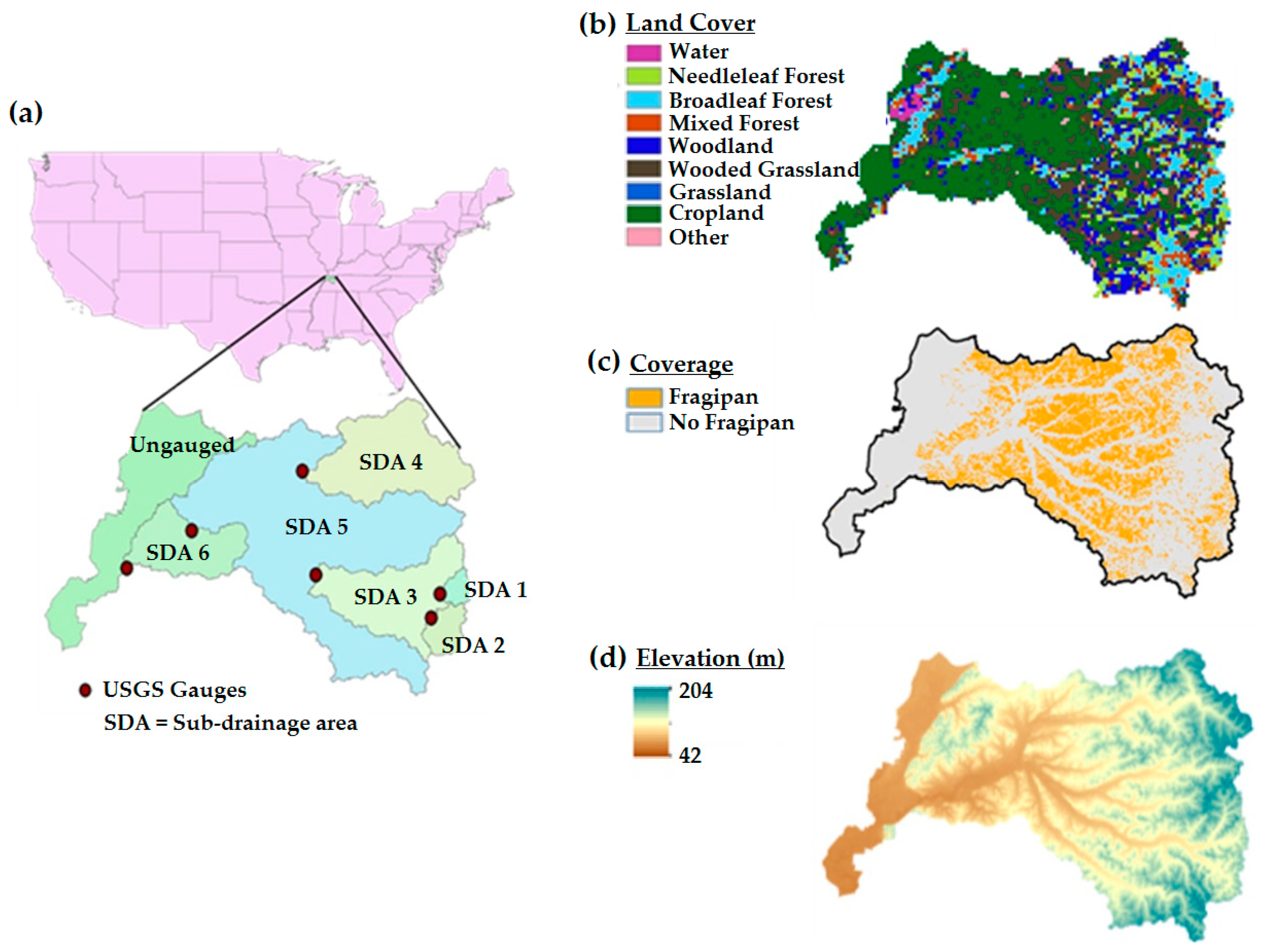
2.1. Study Area

The Obion River Watershed (HUC 08010202-3) is approximately 6400 km² and representative of the lower Mississippi River Basin, which is dominated by row crop agriculture [31] (Figure 2). The ORW has a humid, continental climate and loess-derived soils, making it ideal for agricultural production [32]. As a result, intensive row crop agriculture now dominates the watershed once covered by forest and wooded wetlands. Intensive row crop agriculture and pastured grasslands cover 68.2% of the watershed while forests cover only 28.7%. Residential areas cover the remaining 3.1% (AVHRR land cover data). There are generally two major crop rotations in the cultivated areas; corn-soybean with winter wheat planted as a cover crop or as a double crop, and continuous cotton. Approximately 80 to 90% of the management is continuous no-till.

The annual average precipitation in the watershed is approximately 1310 mm. The majority of the rain occurs in the spring and winter, although heavy convective thunderstorms occur in the summer. The annual average temperature is 14.5 °C. During summer, ET can become the dominant flux in the hydrologic cycle, exceeding incoming precipitation.

The topography and soil properties of the watershed transition from its eastern boundary to the western boundary, which borders the Mississippi River (Figure 2). Rolling topography in the eastern headwaters contain several North-South bands of sand and clay formations. The local streams in this region have a moderately high gradient over generally sandy substrates. Loess plains in the middle of the watershed have a gently rolling topography and contain sand, clay, silt, and lignite capped by loess that can be 50–60 feet thick, generally deeper in the bluff regions towards the West. Streams in this part of the watershed are low-gradient and murky, with silty sand bottoms. Many of the streams have been deforested for agricultural purposes. Channel plugs have formed where aggradation and driftwood accumulate to form blockages and alter flow patterns. Along the Mississippi alluvial plain on the West, there are predominantly clayey soils with poor drainage that may contain wooded swampland and oxbow lakes. Most of the very large farms in ORW exist along the Mississippi River, with smaller farms located in other areas of the watershed.

Fragipan soils cover approximately 30% of ORW [33]. These soils are mostly found in the uplands of the Eastern three-fourths of the watershed (Figure 2). The depth to the fragipan layer in ranges between 0.1 m and 2.0 m below the surface. In most locations, the fragipan layer is below historical tillage depths, typically 30 cm, and is therefore intact [34,35,36]. Furthermore, no-till practices are currently practiced throughout the watershed to prevent additional disturbances to the fragipan layer. The thickness of most fragipan soils is at least 15 cm [24]. The saturated hydraulic conductivity of the fragipan layer in ORW, based on the U.S. Natural Resources Conservation Service (NRCS) soil survey, is around 7 mm/h. The combination of poor drainage and relatively shallow depth to the fragipan layer creates a very flashy hydrologic system [37], especially during more intensive rainfall events, in areas where the fragipan soils are close to the surface.

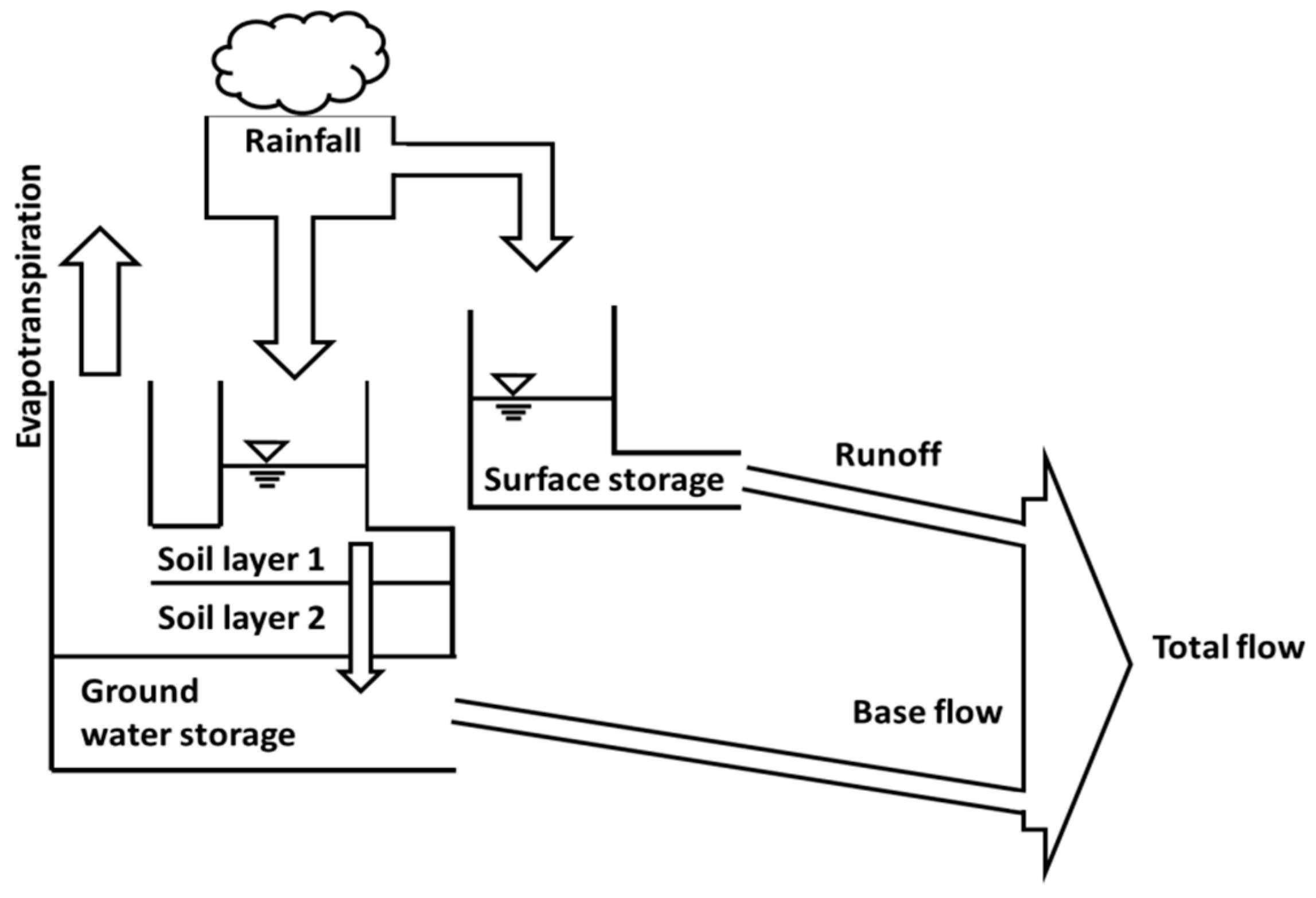
2.2. Hydrologic Model

The three-layer variable infiltration capacity (VIC) model [14,38] was used for this study. VIC has been extensively calibrated and applied for a variety of applications on water resources management, land-atmosphere interactions, and climate change in many large and small basins over the U.S. and worldwide [10,11,12,13,39,40,41,42,43]. Over the past two decades, VIC has been used in several multi-institutional projects such as Project for Intercomparison of Land surface Parameterization Schemes (PILPS) and the North American Land Data Assimilation System (NLDAS) project, and has been shown to compare well with other land surface models and available observed data [18,44,45].

The VIC model framework is described in References [14,46]. VIC balances the water budget within individual grid cells (Figure 1), while considering multiple soil layers with variable infiltration and non-linear base flow. The soil characteristics are defined for each cell and held constant over time. One or more vegetation tiles describes the surface of each grid cell, and the vegetation characteristics such as Leaf Area Index, albedo, resistance, roughness root depth, and its relative fraction in each soil layer, are assigned for each tile. The top two soil layers represent the dynamic response of soil to infiltration. The model allows diffusion between the layers depending on the relative wetness. The model estimates ET using the Penman-Monteith equation. Moisture from the middle layer reaches the bottom layer through gravity drainage, which is regulated by a Brooks-Corey relationship. The bottom layer represents seasonal soil moisture responses except when the other soil layers are saturated. The base flow is only from the bottom layer and is based on the Arno model.

In this study, VIC was run at a daily time step in the water balance mode and results were aggregated at a monthly scale. A grid cell size of 1 km² was adopted to match the Advanced Very High Resolution Radiometer (AVHRR) land cover data used in the study, yielding a total of 6417 cells. For each cell and time step, VIC computed water balance components such as runoff, evapotranspiration, soil moisture, and base flow (Figure 1).

2.3. Data Sources

ORW has a wealth of in-situ and remotely sensed data available for model development, calibration, and validation. The University of Tennessee Institute of Agriculture’s Research and Education Center (REC) at Milan was a primary source of watershed and land-use parameters, as well as measurements of ET and soil moisture. Since 1962, the Milan station has been an active research facility in the heart of the watershed focusing on soil conservation, no-till agriculture, cover crops, and irrigation.

In addition to the REC data, six U.S. Geological Survey (USGS) stream gages within the watershed provided daily streamflow records for at least several years and up to several decades. Additional monthly ET data were obtained from the USGS Simplified Surface Energy Balance (SSEBop) data products [47], downloaded from the Geo Data Portal (https://cida.usgs.gov/gdp/). SSEBop combines reference ET values (from the Penman-Monteith equation) with remotely sensed thermal and vegetation imagery from the Moderate Resolution Imaging Spectroradiometer (MODIS) satellite to generate actual evapotranspiration (AET) data. Soil moisture measurements were also obtained from nearby sites in the NRCS Soil Climate Analysis Network (SCAN). A 30-m Digital Elevation Model of the watershed was obtained from the Tennessee GIS data server (http://www.tngis.org/elevation.htm), and resampled to a 1 km resolution to match the model grid-cell size.

The observed historical climate data used in the study were obtained from DAYMET (http://daymet.ornl.gov/) [48] for 1980–2011, at a spatial resolution of 1 km × 1 km. The weather parameters used included daily precipitation, minimum and maximum temperatures, humidity, and shortwave radiation. Modeled historical and future climate data were also used in the study. These were obtained from the fifth phase of the Coupled Model Intercomparison Project (CMIP5) [49], which provides long-term (hindcast/forecast) climate simulations for 1850–2205 with atmosphere-ocean global climate models (AOGCMs) coupled with Earth system models of intermediate complexity. The historical period of CMIP5 simulations ends in 2005 and the projection begins in 2006. For this study, data was obtained for 1980–2005 for the historical period and for 2006–2050 for the projection period.

Two Representative Concentration Pathways (RCPs) [50], RCP 4.5 and RCP 8.5, were considered for future climate projections. RCP 4.5 is a moderate climate scenario, where an additional radiative forcing of 4.5 W/m² compared to preindustrial conditions will be trapped in the atmosphere by 2100 RCP 8.5 is an extreme climate scenario, where an additional 8.5 W/m² will be trapped by 2100 relative to preindustrial conditions. For each RCP, climate predictions from the following four Global Climate Models (GCMs) were used: (1) The National Oceanic and Atmospheric Administration—Geophysical Fluid Dynamics Laboratory model (GFDL-ESM2M), (2) the Met Office Hadley Centre model (HadGEM2-CC), (3) the Institut Pierre-Simon Laplace model (IPSL-CM5A-MR), and (4) the Japan Agency for Marine-Earth Science and Technology, Atmosphere and Ocean Research Institute at the University of Tokyo, and National Institute for Environmental Studies model (MIROC-ESM-CHEM).

2.4. Model Calibration & Validation

2.4.1. Selection of Calibration Parameters

A calibration process is presented herein for ORW based on its physical characteristics. The study builds on the Troy et al. work [19], which showed that calibration for hydrological modeling (at a spatial resolution of 1/8) using seven key parameters within an allowed range could significantly improve the model results for the conterminous U.S. These seven parameters are presented in

Table 1. Description and determination method of model parameters ¹.

Parameter	Allowed Range	Unit	Determination in This Study	Selected Values for Calibration
b	0.001–1.00	-	Horton model, effective soil moisture approach	-
Ds	0.001–1.00	-	Calibrated	0.1–0.9
Dsmax	0.100–50.00	mm/d	Ksat × Slope 2	-
Ws3	0.200–1.00	-	Calibrated	0.5–0.9
Layer 2 Depth	0.1–3.0	m	Constant	-
Layer 3 Depth	0.1–3.0	m	Sensitivity Analysis	-
Exp	0.1–30.00	-	3 + 2b1 4	-

¹b is the variable infiltration curve parameter, D_smax is the maximum base flow velocity, D_s is the fraction of D_smax where nonlinear base flow begins, W_s is the fraction of maximum soil moisture content above which nonlinear base flow occurs, the Exp parameter characterizes the variation of saturated hydraulic conductivity with soil moisture, and the other two parameters are the depths of 2nd and 3rd soil layers; ² Average slope of cell; ³ W_s > D_s; ⁴ b₁ is slope of soil retention curve as used in Campbell’s equation [51].

along with the ranges adopted in Reference [19]. The method of determination of each of the parameters in this study is also specified in the table.

For small-scale hydrological modeling, heterogeneity within sub-drainage areas should be considered in calibration for better representation of the watershed. The fine spatial resolution (1 km² grid cell) employed in this study provided the basis to account for the heterogeneity. Properties of each cell such as soil, vegetation, and climate were determined and assigned accordingly to represent the watershed heterogeneity.

According to Reference [14], the b-parameter has the largest effect on runoff, while the D_s and W_s parameters are critical in influencing the baseflow. Estimation of these three parameters is thus crucial for model performance. Unlike the other four parameters (i.e., D_smax, Exp, and depths of soil layers 2 and 3), which are readily obtained from soil maps, b, D_s, and W_s are usually calibrated since they are generally unknown and can vary considerably within a watershed [52]. In this study, b was estimated using soil data and Horton’s infiltration relationship [30], while D_s and W_s were estimated by evaluating plausible physical values for both parameters. The parameters D_smax and Exp were also calculated using empirical relationships (see Table 1). The depths of the second and third soil layers were chosen to be consistent with the soil layers of the CONUS-Soil data [53]. For the third layer, however, a sensitivity analysis was further performed to determine a minimum required depth of 1.4 m. Cells with layer 3 depths lower than this value had fast drainage and unrealistically low soil moisture contents.

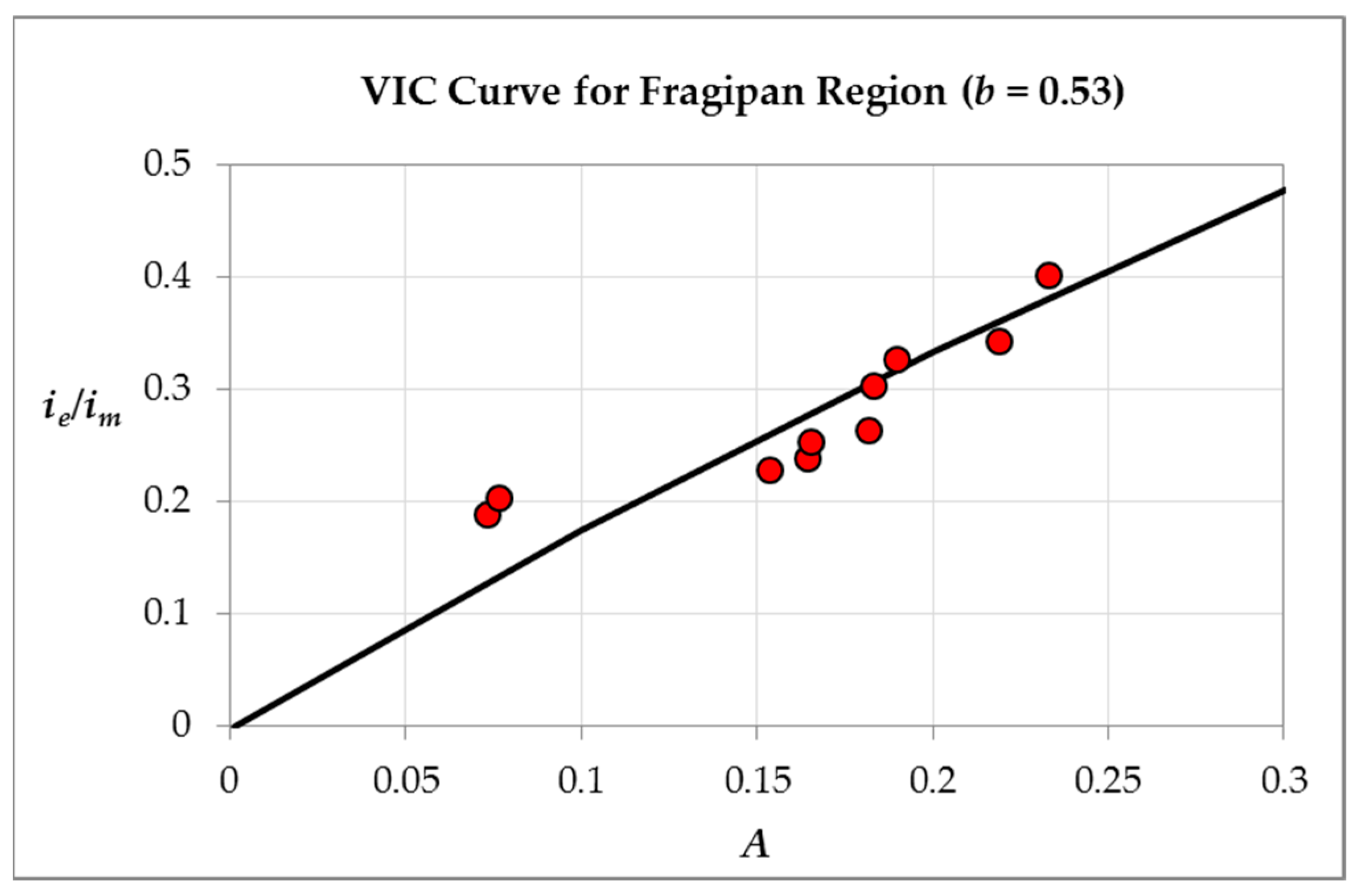
2.4.2. Estimation of Calibration Parameters

As discussed above, the b-parameter is an important model parameter and should be determined carefully to make sure that model results are physically meaningful. Based on its definition, b controls the partitioning of rainfall into runoff and infiltration, and ranges commonly between 0 and 0.4, though larger values have been estimated for some watersheds [19,54]. Higher values produce more runoff and less infiltration whereas lower values produce less runoff and more infiltration. An extensive literature search for the parameterization of the b-parameter (see

Table A1. Treatment of b parameter in various VIC studies.

Article	Model Size	Value	Definition	Method
Zhao et al. [72]	N/A	0.2–0.4	Topographic factor, denoting non-uniformity of distribution of soil moisture storage. b = 0.2–0.4 for mountainous and hilly areas.	First estimated directly from observed hydrological data and then calibrated in the computation routine
Zhao [73]	N/A	0.1–0.4	Defines the non-uniformity of the surface conditions. (<10 km2), b = 0.1 and basins (<1000 s km2), b = 0.4. As x moves down the curve, it implies a redistribution of soil moisture during the drying period, with water flowing from the more elevated parts of the sub-basin to the lower parts.	Experience
Dumenil and Todini [74]	600 km × 600 km	0.01–0.5	Parameter b is a function of orography only	Orography correction to represent steep orography
Wood et al. [15]	767 km2	0.01–10; 0.085–0.129	Shape parameter. Acknowledges that model assumes infiltration capacities vary within an area due to variations in topography, soil, and vegetation.	Sensitivity Analysis Estimated
Liang [14]	11.7 km2	0.008	Infiltration shape parameter	Estimated from streamflow, precipitation, and maximum/minimum temperature through calibration.
Kalma et al. [75]	26 km2	4	Empirical parameter	Assumed that they had a set of total storage capacity values. The cumulative frequency of these values were plotted and then was fit with different values of b by trial and error.
Zhao and Liu [76]	N/A	0.1–2	b varies from 0.1–0.4 when spatial scale is within thousands of square kilometers. b increases significantly to 1 or 2 even more when modeling area is over tens of thousands of square kilometers. b reflects the pattern of land surface characteristics (<100 km2) and heterogeneity of the land surface and distribution of rainfall (<1000 s km2)	Experience and through calibration of precipitation and streamflow.
Sivapalan and Woods [10]	N/A	4.03	Empirical parameter	Through fitting a distribution of soil depths obtained through field observations.
Liang et al. [46]	N/A	0.01–0.5—Based off range from Todini 1992	Infiltration shape parameter which is a measure of the spatial variability of the infiltration capacity.	Estimated using hydrologic information (especially streamflow). If no information is present, determine based on past calibration experience.
Abdulla et al. [58]	1 × 1 degree	0–0.4	Infiltration parameter	Estimated using the Shuffled Complex Evolution search method where the objective function was the sum of squared differences between the simulated and observed streamflow. This was then spatially interpolated to derive b values across the basin.
Lohmann et al. [18]	1/6 degree = 18 km	0.12–0.16	Infiltration capacity shape parameter	Calibrated through requiring direct runoff to approximately equal the fast flow from the routing model in VIC.
Jayawardena and Zhou [77]	131 km2	13.186 (single parabolic curve)	Measures the non-uniformity of the spatial distribution of the soil moisture storage capacity over the catchment.	Calibrated using daily hydrological data
Nijssen et al. [78]	1 degree 0.5 degree	0.1–0.25	Infiltration parameter	Estimated manually by comparing naturalized monthly streamflow hydrographs with modeled monthly hydrographs at key locations.
Liang and Xie, [79]	1/8 degree cells	0.1–0.5	Soil moisture capacity shape parameter, which is a measure of the spatial variability of the soil moisture capacity, defined as the maximum amount of water that can be stored in the upper layer of the soil column. It is a surrogate for spatial heterogeneity of soil properties.	Sensitivity Analysis Meant to represent moderate infiltration capabilities.
Woolridge et al. [80]	Lumped—1260 km2 Distributed	3.68–5.32; 2.069–7.20	Model parameter giving the concave up shape for values less than one and convex up for values greater than one.	Optimized from rainfall-runoff data
Huang and Liang [20]	N/A	0–13.5, however, only kept values 0–5	Controls the shape of the spatial distribution of soil moisture capacity over a study area, and thus plays a significant role in describing the heterogeneity of soil moisture capacity over the study area. Derived from STATSGO data.	Estimated from STATSGO database. Estimated by fitting distribution of calculated soil moisture capacity of each soil column (soil moisture capacity = total soil depth × soil porosity).
Xie and Yuan [59]	32–370 km2 (treated as lumped units)	0.15–0.45	Infiltration parameter which controls the amount of water that can infiltrate into the soil.	Calibration between observed and modeled hydrograph
Xie and Yuan et al. [81]	50 km2	0–10	Infiltration parameter which controls the amount of water that can infiltrate into the soil.	Calibration using streamflow
Chen et al. [82]	N/A	0–larger	Represents the spatial heterogeneity of spatial field capacity (b = 0 for uniform distribution and large for significant spatial variation)	Calibration using streamflow and precipitation data.
Oubeidillah et al. [9]	4 km × 4 km	0.001–0.8	Variable infiltration curve parameter	Calibration of modeled streamflow against USGS Water Watch data for each HUC8 in CONUS

in the Appendix A) reveals two readily noticeable facts: (1) The range of values used in the literature is wide; and (2) there is a lack of a consistent methodology used to derive this parameter. Sivapalan and Woods [10] and Huang et al. [20] are two of the few studies that have attempted to determine b directly from soil observations. However, as explained in the introduction, a shortcoming of these studies is the assumption of a static soil moisture capacity distribution, which is not directly applicable to watersheds with distributions of fragipan soils that vary in space, both laterally and with depth. To address this issue, this study adopts a dynamic or effective soil moisture capacity distribution assumption for determining the value of b.

Since fragipan layers regulate infiltration, leading to perched saturation zones and increased runoff [55], the effective soil moisture capacity for fragipan regions is estimated herein with the following relationship derived from integration of Horton’s curve:

i_e = f_ct_s − (f₀ − f_c)e^−kts/k,

(1)

where i_e is the effective soil moisture capacity (L), f_c is the final constant infiltration capacity, i.e., saturated hydraulic conductivity (LT⁻¹), f₀ and k are, respectively, the initial infiltration capacity (LT⁻¹) and decay rate (T⁻¹) and t_s is the time to steady infiltration (T). Equation (1) accounts for dynamic or temporal effects that control water storage and saturation in the soil. Field data for fragipan sites within the watershed were used to determine the variables on the right hand side of Equation 1, from which i_e was then computed. The computed values of i_e across the watershed were used to establish the cumulative soil moisture capacity curve, from which b was determined by fitting the following distribution [54]:

i_e = i_m [1 − (1 − A)^1/b],

(2)

where i_m is the maximum soil moisture capacity (L), and A is the fraction of the area for which the infiltration capacity is less than i_e. Further details on the estimation of i_e and b for ORW is provided below.

For the fragipan areas in the watershed, values of f₀ and k averaged 210 mm/h and 2 min⁻¹, respectively [56]. The average f_c value for fragipan soils, based on the NRCS soil survey, was also approximately 7 mm/h. The t_s determined from field experiments was on average 60 h for an approximate soil depth of 2 m, with fragipan soils occurring around 600 mm below the surface. Using Equation (1), an average i_e value of 432 mm could then be estimated for the fragipan regions (i.e., an effective soil moisture capacity approximately 51% of the total capacity of the soil column, which has a porosity of 0.42). Repeating the step for different fragipan depths, the cumulative distribution of effective soil moisture capacities were plotted and Equation (2) was fitted to the data to obtain an estimate of 0.53 for the b value. This is shown in Figure 3. Following a similar approach, a b value of 0.04 was determined for the non-fragipan regions.

Since VIC requires a single value of b per grid cell, it was necessary to determine an effective b value for each cell based on the relative influences of fragipan and non-fragipan areas within the cell. This required a sensitivity analysis of the b-parameter to determine first whether or not variations in b had a significant impact on rainfall-runoff-baseflow flux proportioning, and then to determine its relationship with the runoff coefficient (i.e., ratio of runoff to rainfall) to establish weighting factors for computing the effective b value from the fragipan and non-fragipan b values and area proportions. As mentioned above, fragipan soils cover approximately 30% of ORW. However, the actual proportion of fragipan to non-fragipan area within each grid cell will vary from cell to cell depending on the landscape characteristics [57]. For the sake of simplicity, an assumption of 30% fragipan coverage was made for each grid cell falling within a sub-drainage areas where fragipan soils were present. Since the VIC flux predictions are aggregated herein to the sub-drainage scale, this assumption is valid because fragipan effects at that scale are aggregated in reality and will reflect the approximate coverage in each sub-drainage area.

The sensitivity analysis was performed for a two-year period (2010–2011). The b-parameter was varied between 0.15 and 0.9 and its effects on the runoff, baseflow, and streamflow were analyzed. The results are presented in Figure 4 along with the simulated precipitation. As seen, higher b values produced more runoff (Figure 4a) and less baseflow (Figure 4b). For streamflow, this resulted in higher hydrograph peaks and lower troughs (Figure 4c). Overall, runoff differed by as much as 150% (a factor of 2.6) in May of the first year, while baseflow differed by as much as 170% (a factor of 2.7), indicating a sensitivity of the water fluxes to the value of the b-parameter. In terms of streamflow, the differences in peaks were only as much as 50% (a factor of 1.5) in May of the first year while differences in troughs were only as much as 100% (a factor of 2) in August of the first year. Given the large difference between the estimated b-parameter for fragipan (~0.53) and non-fragipan regions (~0.04) in ORW, the sensitivity analysis suggests that the separate estimation for fragipan and non-fragipan areas is justified since significantly different responses in terms of runoff, baseflow, and streamflow are expected.

The relationship between the b-parameter and the normalized runoff coefficient is plotted in Figure 5 based on the sensitivity analysis results (each dataset is normalized with the runoff coefficient corresponding to b = 0.9). The overall trend for the mean runoff coefficient (solid red line in Figure 5) follows an approximate power law (Hoerl curve). Using this relationship, an effective normalized runoff coefficient of 0.4 was estimated for a cell with 30% fragipan (b = 0.53) and 70% non-fragipan (b = 0.04) coverage. From this effective normalized runoff coefficient value, a corresponding effective b parameter of 0.15 was estimated, which was adopted in the model.

The common ranges of D_s and W_s adopted from the literature are, respectively, 0.001–1 and 0.2–1 [9] (see

Table 2. Physical ranges for calibration parameters adopted in past studies.

Study	Watershed Area	Cell Size	Time Step	Region	Soil Order 1	Fragipan	Hydrological Regime	Land Cover	b	Ds	Ws
Liang et al. [14]	11.7 km2	15 km	Daily	King Creek, Kansas	Mollisols	No	Semiarid	Tall Grass	0.008	7.7 × 10−5	0.96
Abdulla et al. [58]	6 × 105 km2	1 degree	Daily	Arkansas-Red River (US Southern Great Plains)	Utisols, Alfisols, Mollisols	Yes, on eastern side of basin	Arid to Humid	Grass, Shrub, Woodland, Forest, Alpine	0.0–0.4	-	-
Troy et al. [19]	Cell-Based	1/8 degree	12 h	Northwest Tennessee	Alfisols	Yes	Sub-humid to Humid	Crop, Grass	0.2–0.5	-	-
Xie and Yuan [59]	43–371 km2	Each watershed treated as one cell	Hourly	France (12 Watersheds)	Alfisols, Inceptisols	Yes, on eastern side of France	Humid	Forest, Woodland, Grass, Shrub, Crop	0.15–0.45	0.02	0.8
Chawla and Mujumdar [52]	9 × 104 km2	1/2 degree	Daily	Midstream Upper Ganga Basin, India	Lithosols, Cambisols, Regosols, Gleysols, Fluvisols	No	subequatorial monsoon climate with sufficient moistening	Forest, Crop	0.044	0.0004	0.62

¹ Soil orders are based on the USDA classification system, except for [52] which is based on the FAO classification.

). The selected values for calibrating D_s, and W_s used in this study (presented in Table 1) were chosen after reviewing the literature for VIC simulations of regions close to west Tennessee or with relatively similar soil and/or hydrological regime to ORW (see Table 2).

Based on the soil properties, model parameter values for D_smax ranged from 0 to 100 for the 6147 cells, with an average value of around 10. Likewise, parameter values for Exp ranged from 3 to 20, also with an average value of around 10. Finally, the depths of the 2nd and 3rd layers generally fell between 0.4 m and 1.5 m.

3. Results

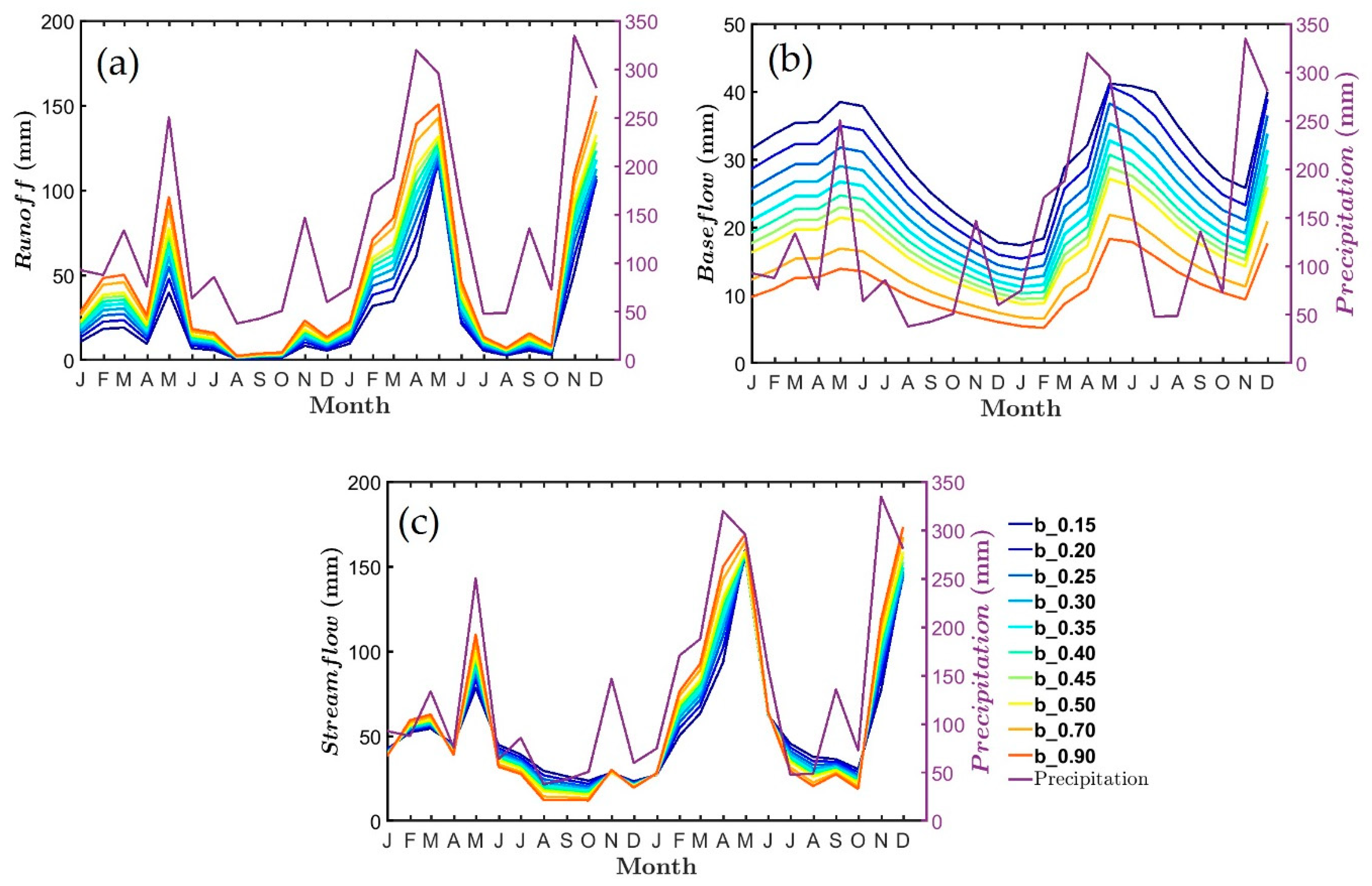
3.1. Model Calibration

The model was calibrated by comparing simulated monthly streamflow fluxes for each of the six SDAs (Figure 2) against corresponding observed monthly USGS streamflow data for the period of 1980–2011. Relative bias and the Nash-Sutcliffe efficiency coefficient [60] were used as the measures of performance for each calibration case. The best set of calibration parameters and model performance values for each SDA, along with the USGS gauging stations used, are presented in

Table 3. Streamflow calibration: Nash-Sutcliffe Efficiency (NSE) Coefficient and Relative Bias for the best combination of calibration parameters each Sub Drainage Area (SDA).

SDA	Ds	Ws	NSE Coef.	Relative Bias	USGS Station
1	0.9	0.9	0.71	0.23	07024200
2	0.9	0.9	0.74	0.10	07024300
3	0.9	0.9	0.67	0.32	07024500
4	0.1	0.5	0.75	0.04	07025400
5	0.9	0.9	0.73	0.12	07026040
6	0.9	0.9	0.73	0.16	07026300

. A comparison between simulated streamflow hydrographs and corresponding USGS streamflow hydrographs for two of the SDAs is also shown in Figure 6. As seen, the calibrated model correctly predicts the overall trends in streamflow and captures well the low flows. However, it tends to underestimate high peak flows. The Nash-Sutcliffe Efficiency coefficient above 0.65 for all SDAs suggests that the model results are good [61,62,63].

The effective soil moisture capacity approach used herein for determining b gives confidence that the model is able to partition correctly precipitation to infiltration and surface runoff. To validate the model’s ability to simulate and partition subsurface fluxes, the calibrated results were also compared with observed data of AET and soil moisture. Figure 7 compares the MODIS-derived AET with the VIC-simulated AET for the entire watershed from 2000 to 2012. As seen, the MODIS values are generally within one standard deviation of the VIC values and the Nash-Sutcliffe efficiency coefficient is 0.77, which suggests good agreement. Furthermore, the simulated AET values are also similar to the average range of 25–125 mm per month reported for the Arkansas-Red River basin (which neighbors ORW on the west) in Reference [58].

Figure 8 shows the comparison between the simulated and observed soil moisture data from 2004 to 2010. The observed data in this case are field observations obtained from the NRCS-SCAN network. The comparison confirms that the model was able to replicate the magnitude and trends in soil moisture in the watershed, with a fair Nash-Sutcliffe Efficiency Coefficient of 0.4.

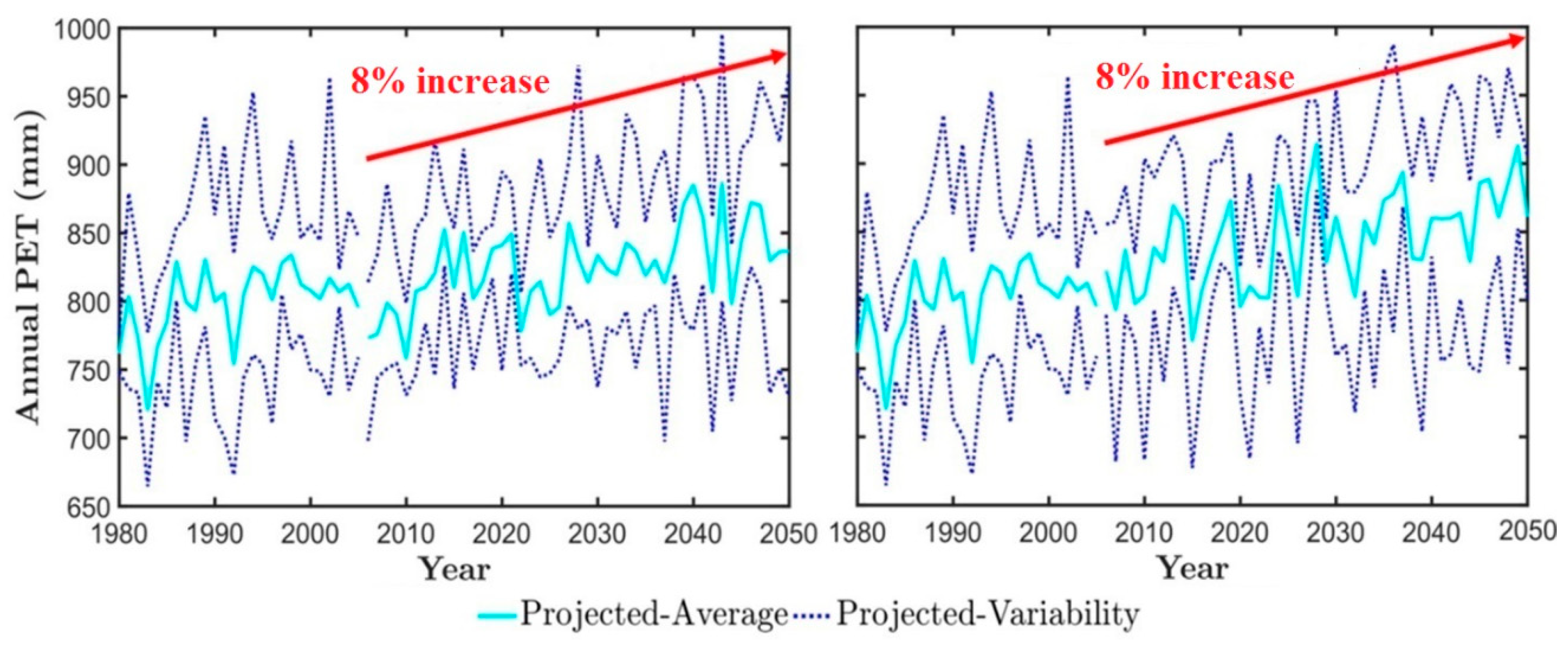
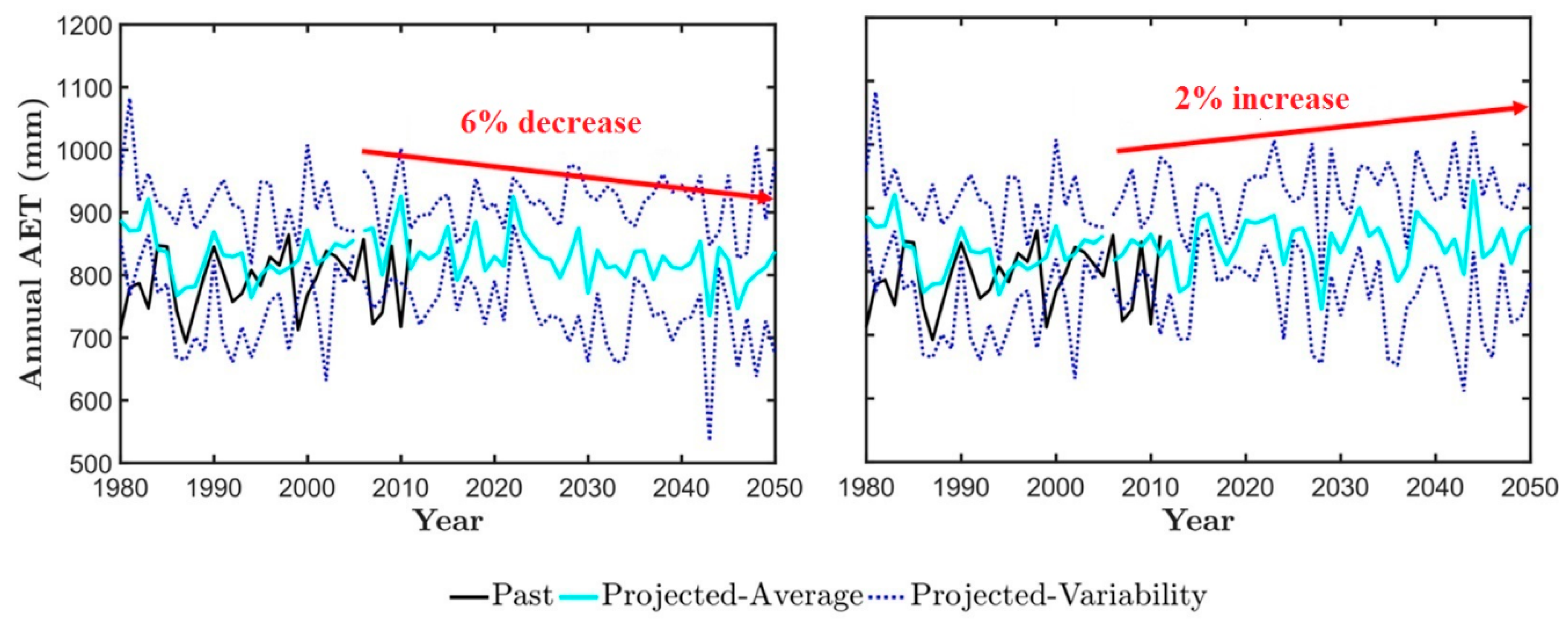
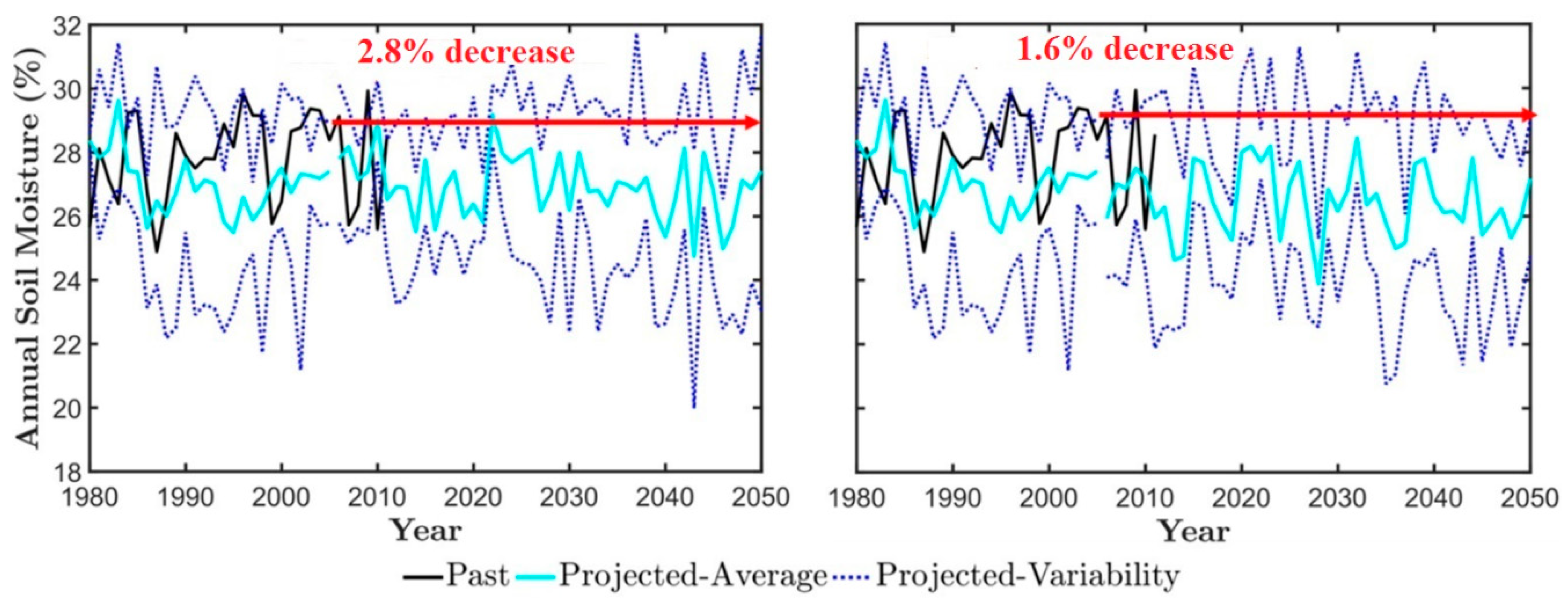
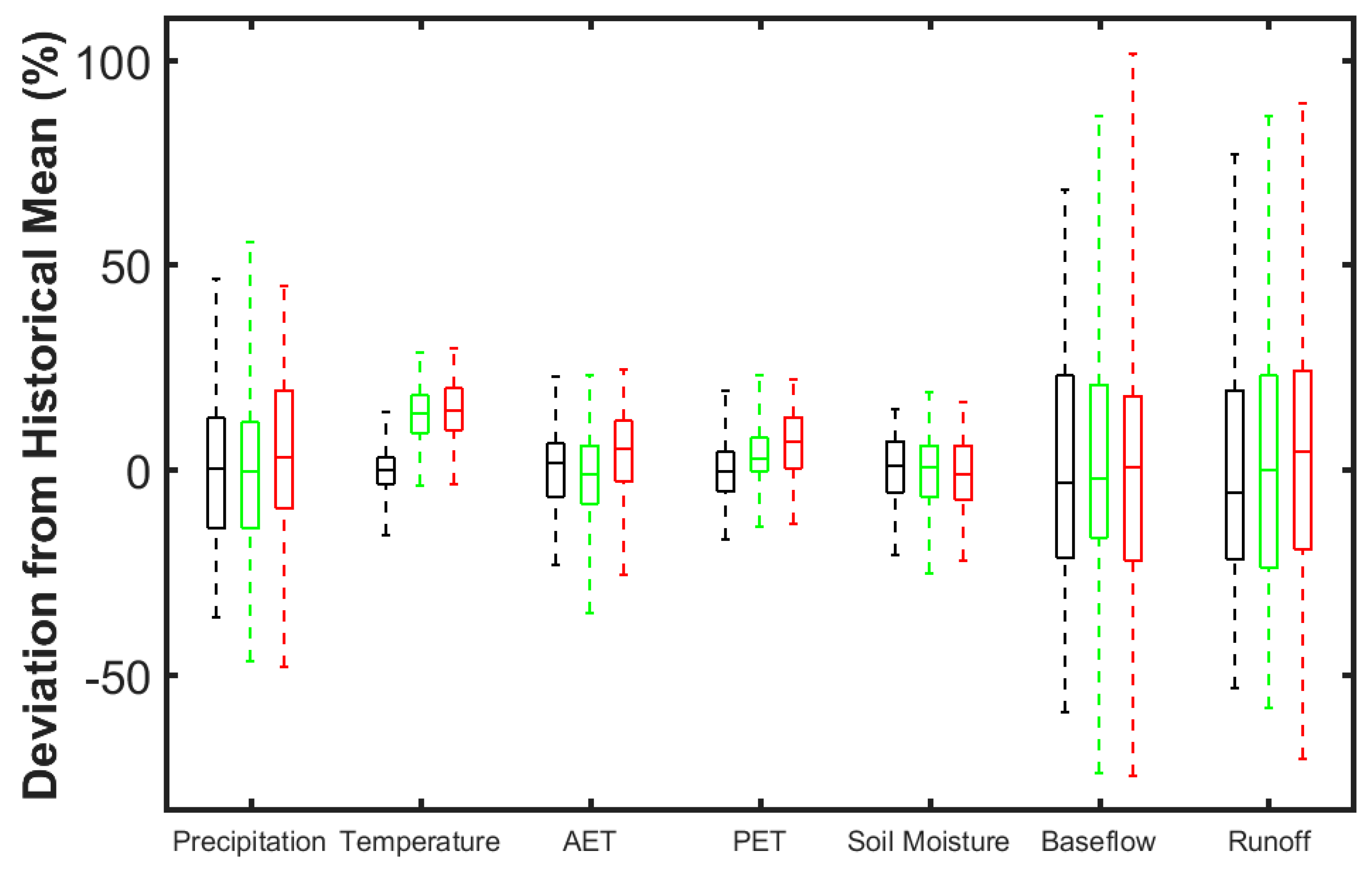
3.2. Climate Impact on the Obion River Watershed Water Budget

Figure 9 presents annual precipitation and temperature time series in ORW for the historical and projection periods examined herein. In each plot, the dotted blue lines represent the maximum and minimum model predictions (among all four GCMs), and the solid black curve shows the observed historical data. The solid cyan line is the ensemble average of the four GCMs.

While there are no obvious trends in precipitation for both the RCP 4.5 and RCP 8.5 scenarios, RCP 4.5 shows a slight decline, whilst RCP 8.5 shows a slight increase. This is accordance with reported trends for the region for the 20th century. According to Hanson and Weltzin [64], the region had about a 1% increase of precipitation per decade over a 100-year period. It was also reported that the number of moderate and extreme dry months (according to the Palmer Index) in the second half of the same 100-year period was less than the first half [64].

On the contrary, historic and projected temperatures clearly exhibit a rising trend with an approximate increase of 3 °C over the 70-year period from 1980 to 2050, for both RCP 4.5 and RCP 8.5 scenarios. Consistent with these are the annual time series of potential evapotranspiration (PET), which also show an increasing trend for both RCP 4.5 and 8.5 till 2050 (~1.4 mm/year), with no significant differences between the scenarios (see Figure 10). This is to be expected since PET is a function of the mean temperature, among others.

Unlike PET, the annual time series of AET show different trends (see Figure 11). While the projected AET for RCP 8.5 is increasing, the projected AET for RCP 4.5 is declining. This phenomenon can be explained by the precipitation trends shown in Figure 8. Consistent with AET trends, the projected precipitation declines for RCP 4.5 and rises for RCP 8.5. Studies indicate that changes in wind and air temperature may not always be the root cause for AET changes, and that changes in precipitation characteristics can dominate AET trend changes [65]. The decline in precipitation for RCP 4.5 results in a soil moisture limitation that primarily drives declines in the ET [66]. Thus, the available water restricts variation of AET for this region in West Tennessee.

Figure 12 shows the soil moisture time series for the historical and projected periods. The projected time series for both RCPs are within the same range as the historical period. In addition, the slope of the trend for both RCPs is negligible, suggesting no significant changes due to climate in the near future till 2050. It is worth noting that variation of soil moisture through ET also depends on land use/land cover [67]. In this study, the land use/land cover was fixed to current values for the projection period. Any land use/land cover changes in future may directly affect ET, and consequently the soil moisture.

The above trends for precipitation, temperature, PET, and AET, along with trends in runoff and baseflow, are summarized in Figure 13. Box plots of the parameters for the historical period are compared to the associated box plots projected for RCPs 4.5 and 8.5. The comparisons are for the 20-year periods of 1986–2005 in the past and 2031–2050 in the future. For comparison purposes, all parameters are presented as deviations from the average value during the historical period. Precipitation and temperature are known drivers of change in the water balance. For ORW, while there are slight changes in precipitation, there are significant changes in the temperature for the projected period. However, as noted previously, the water balance in this region is more restricted by water availability. Therefore, the projected changes in the other water budget parameters, including AET, soil moisture, baseflow, and runoff are slight, except some changes in the most extreme data points manifested by extension of the whiskers in Figure 13.

Statistical tests were used to assess quantitatively changes in the mean and standard deviation of each parameter from the historical period to the projected period. The same 20-year periods considered in Figure 13 were used for these tests. T-tests were used to measure differences in the mean while F-tests were used to compare standard deviations. The results of the tests are presented in

Table 4. Statistical comparison of average annual fluxes for two 20-year periods of 1996–2005 (historical) and 2031–2050 (projected; RCP 4.5 and RCP 8.5). Results of 0 and 1 show, respectively, statistically insignificant and significant changes (significance level 0.01). The statistically significant changes are highlighted in bold.

Parameter	Mean			Standard Dev.			T-Test				F-Test
	Past	RCP 4.5	RCP 8.5	Past	RCP 4.5	RCP 8.5	RCP 4.5		RCP 8.5		RCP 4.5		RCP 8.5
							Result	p-Value	Result	p-Value	Result	p-Value	Result	p-Value
Precipitation (mm)	1308	1316	1350	231	278	254	0	0.84	0	0.28	0	0.10	0	0.40
Temperature (°C)	14.91	16.93	17.09	0.84	1.01	1.17	1	2 × 10−28	1	2 × 10−27	0	1 × 10−1	1	4 × 10−3
AET (mm)	820	812	851	81	90	89	0	0.57	0	0.02	0	0.33	0	0.40
PET (mm)	809	840	860	57	63	67	1	9 × 10−4	1	5 × 10−7	0	4 × 10−1	0	2 × 10−1
Soil Moisture (%)	26.7	26.7	26.4	2.3	2.4	2.4	0	0.95	0	0.41	0	0.67	0	0.62
Baseflow (mm)	303	311	303	89	98	97	0	0.59	0	0.97	0	0.35	0	0.41
Runoff (mm)	185	191	192	52	65	58	0	0.50	0	0.39	0	0.05	0	0.35

. Only two parameters, i.e., temperature and PET, show significant changes in their mean values into the projected period for both RCP 4.5 and RCP 8.5. Further, the only parameter that shows a statistically significant change in its standard deviation is the temperature for RCP 8.5. The findings suggest that there will be a significant increase in extreme temperature conditions under the RCP 8.5 scenario. Overall, however, the statistical results suggest that changes in projected water budget will be not significant in near future for the ORW.

The characteristics of ORW were also examined with the Budyko curve [68], which is a common representation of the land-water balance that describes the mean-annual partitioning of precipitation into streamflow and evaporation. The curve summarizes the relation between the ratios of AET/P (evaporative index) and PET/P (dryness index), where P is precipitation. The distribution of annual values on the Budyko curve (Figure 14) can be used to determine the following characteristics of a watershed [69]:

• Resistance (or responsivity), which measures the degree to which streamflow is synchronized with precipitation, and;
• Resilience (or elasticity), which measures the degree to which a watershed can return to normal functioning following perturbations.

Resistance was estimated from the deviation in the AET/P of annual values (i.e., Δy-axis), while resilience was estimated as the ratio of deviation in PET/P to the deviation in AET/P (i.e., Δx-axis/Δy-axis). The data suggest that ORW has a relatively low resistance (i.e., high responsivity = 0.9), meaning that streamflow is largely synchronous with precipitation. This result is consistent with the effects of the fragipan soils in the region, which systematically transfers precipitation into streamflow discharge with less storage. Further, the ORW has a high resilience (i.e., elasticity = 2.3 (> 1)), so it has the capacity to sustain its functionality after extreme climatic perturbation such as drought or extreme precipitation [69].

4. Discussion and Conclusions

Biases in streamflow predictions in the U.S. Southeast from past hydrological modeling studies have been attributed to calibration issues [18,19]. Since other regions with similar climate have not shown a similar bias, landscape characteristics are believed to be the cause of the bias. Specifically, the occurrence and extensive coverage of fragipan soils in the region are thought to control hydrologic response by affecting the partitioning of rainfall into runoff and infiltrated water, especially during more intensive rainfall events, in areas where the fragipan soils are close to the surface.

This study presented a methodology for calibrating regions with significant fragipan coverage based on the effective soil moisture capacity associated with these features. Estimation of the b-parameter of the VIC model, which controls rainfall-runoff-infiltration partitioning, was based on fragipan layer characteristics such as the saturated hydraulic capacity, the time to saturation, and the depth to the fragipan layer. This approach avoided the need to evaluate the wide range of b-parameter values recommended in literature (see Table A1) to match the observed flows. Further, since the approach is based on the physical characteristics of the soil, simulated trends in runoff and baseflow, as well as the behavior of the watershed in terms water budget response can be attributed to the processes that take place.

The proposed approach was successfully applied to the Obion River Watershed located in the U.S. Southeast, specifically the Northwestern part of Tennessee. Estimated b-parameter values of 0.53 and 0.04 for fragipan and non-fragipan soils, respectively, in the watershed produced good model predictions with Nash-Sutcliffe coefficient values greater than 0.65 and relative bias values ranging between 0 and 0.32 for sub-drainage areas within the watershed. A sensitivity analysis on the b-parameter validated the need to examine fragipan and non-fragipan soils separately in the watershed and confirmed that fragipan soils were resulting in flashier streamflow response with higher peaks and lower troughs. Further, the calibrated model was also shown to correctly predict trends in evapotranspiration and soil moisture, confirming that it was able to correctly partition subsurface fluxes in the various components.

The calibrated model was used to study the impacts of climate on the water balance in ORW. Water budgets were simulated for past and future projected climates up to 2050 (based on four GCMs for RCPs 4.5 and 8.5). While no significant changes in the water balance were forecasted for the near future (based on T-tests and F-tests), the results suggested a significant change in extreme temperature conditions for the RCP 8.5 scenario. Trends in the fluxes also suggested that the water budget in ORW is controlled to a large degree by water availability. This explains the lack of sensitivity of the water budget to forecasted temperature increases. The effect of a temperature increase will be to increase PET. However, since water availability is limiting, the AET will be regulated by the water input (i.e., precipitation) and not temperature [66], thereby rendering the watershed less sensitive to temperature changes. Being a cropland, this scenario occurs primarily during the growing season in ORW when most of the ET occurs. Nonetheless, the effects are reflected in the annual water budget trends since ET is the primary system water output on an annual basis (see Table 4).

Annual changes in the evaporative (AET/P) and dryness (PET/P) indices of ORW on the Budyko curve were used to characterize its responsivity (i.e., the degree to which streamflow is synchronized with precipitation) and resilience (i.e., the degree to which a watershed can return to normal functioning following perturbations). The ORW was found to have a high responsivity of 0.9, suggesting that stream flow was largely synchronized with precipitation. This finding is consistent with the effects of the fragipan soils in the region, which tends to systematically transfer precipitation into streamflow discharge with relatively less storage. The ORW was also found to have a high resilience of 2.3, also indicating that it has the capacity to sustain its functionality after extreme climatic perturbation such as drought or extreme precipitation.

The projection of no significant changes in the water budget of ORW in the near future has implications to the region’s agriculture. While the irrigation for agricultural purposes in Tennessee has been increasing over past decades and is expected to increase over the next decades [70], it is well below the average in the country. The average acres of farms under irrigation was 17.8% for Tennessee and 25.4% for the United States with average acre-feet irrigation per acre of 0.4 for Tennessee and 1.6 for the United States [71]. Since the mean soil moisture and evapotranspiration are not expected to change profoundly until 2050, agriculture in Western Tennessee can be expected to continue to perform similarly to recent trends, holding economic factors constant. Furthermore, water sources for irrigation are not expected to be impacted in the near future from climate changes according to the projected water balance.

References

1. Rodriguez-Iturbe, I.; Porporato, A. Ecohydrology of Water-Controlled Ecosystems: Soil Moisture and Plant Dynamics, 1st ed.; Cambridge University Press: Cambridge, UK, 2005. [Google Scholar]
2. Al-Kaisi, M.M.; Elmore, R.W.; Guzman, J.G.; Hanna, H.M.; Hart, C.E.; Helmers, M.J.; Hodgson, E.W.; Lenssen, A.W.; Mallarino, A.P.; Robertson, A.E.; et al. Drought impact on crop production and the soil environment: 2012 experiences from Iowa. J. Soil Water Conserv. 2013, 68, 19A–24A. [Google Scholar] [CrossRef]
3. Pack, D.; Robinson, K. About $300 Million in Indiana Crops’ Value Lost to Flooding so Far; Purdue University Agricultural News: Purdue, IN, USA, 2015. [Google Scholar]
4. Ramírez, J.A.; Finnerty, B. Precipitation and water-table effects on agricultural production and economics. J. Irrig. Drain Eng. 1996, 122, 164–171. [Google Scholar] [CrossRef]
5. Clark, C.D.; Harden, C.; Park, W.; Schwartz, J.; Ellis, C.; McKnight, J.; Betterton, E.; Tracy, H.; VanCor, K. The Water-Energy Nexus in East Tennessee; White Paper; University of Tennessee: Knoxville, TN, USA, 2013. [Google Scholar]
6. Ingram, K.T.; Dow, K.; Carter, L.; Anderson, J. Climate of the Southeast United States: Variability, Change, Impacts, and Vulnerability; Island Press: Washington, DC, USA, 2013. [Google Scholar]
7. McCuen, R.H.; Snyder, W.M. Hydrologic Modeling. Statistical Methods and Applications; Prentice-Hall: Englewood Cliffs, NJ, USA, 1986. [Google Scholar]
8. Hejazi, M.I.; Moglen, G.E. The effect of climate and land use change on flow duration in the Maryland Piedmont region. Hydrol. Process. 2008, 22, 4710–4722. [Google Scholar] [CrossRef]
9. Oubeidillah, A.A.; Kao, S.C.; Ashfaq, M.; Naz, B.S.; Tootle, G. A large-scale, high-resolution hydrological model parameter data set for climate change impact assessment for the conterminous US. Hydrol. Earth Syst. Sci. 2014, 18, 67–84. [Google Scholar] [CrossRef] [Green Version]
10. Sivapalan, M.; Woods, R.A. Evaluation of the effects of general circulation models’ subgrid variability and patchiness of rainfall and soil moisture on land surface water balance fluxes. Hydrol. Process. 1995, 9, 697–717. [Google Scholar] [CrossRef]
11. Aggarwal, S.P.; Garg, V.; Gupta, P.K.; Nikam, B.R.; Thakur, P.K.; Roy, P.S. Run-off potential assessment over Indian landmass: A macro-scale hydrological modelling approach. Curr. Sci. 2013, 104, 950–959. [Google Scholar]
12. Wang, G.Q.; Zhang, J.Y.; Jin, J.L.; Pagano, T.C.; Calow, R.; Bao, Z.X.; Liu, C.S.; Liu, Y.L.; Yan, X.L. Assessing water resources in China using PRECIS projections and a VIC model. Hydrol. Earth Syst. Sci. 2012, 16, 231–240. [Google Scholar] [CrossRef] [Green Version]
13. Houborg, R.; Rodell, M.; Li, B.; Reichle, R.; Zaitchik, B.F. Drought indicators based on model-assimilated Gravity Recovery and Climate Experiment (GRACE) terrestrial water storage observations. Water Resour. Res. 2012, 48. [Google Scholar] [CrossRef] [Green Version]
14. Liang, X.; Lettenmaier, D.P.; Wood, E.F.; Burges, S.J. A simple hydrologically based model of land surface water and energy fluxes for general circulation models. J. Geophys. Res. Atmos. 1994, 99, 14415–14428. [Google Scholar] [CrossRef]
15. Wood, E.F.; Lettenmaier, D.P.; Zartarian, V.G. A land-surface hydrology parameterization with subgrid variability for general circulation models. J. Geophys. Res. 1992, 97, 2717–2728. [Google Scholar] [CrossRef]
16. Bowling, L.C.; Lettenmaier, D.P. Modeling the Effects of Lakes and Wetlands on the Water Balance of Arctic Environments. J. Hydrometeorol. 2010, 11, 276–295. [Google Scholar] [CrossRef]
17. Bohn, T.J.; Livneh, B.; Oyler, J.W.; Running, S.W.; Nijssen, B.; Lettenmaier, D.P. Global evaluation of MTCLIM and related algorithms for forcing of ecological and hydrological models. Agric. For. Meteorol. 2013, 176, 38–49. [Google Scholar] [CrossRef]
18. Lohmann, D.; Mitchell, K.E.; Houser, P.R.; Wood, E.F.; Schaake, J.C.; Robock, A.; Cosgrove, B.A.; Sheffield, J.; Duan, Q.Y.; Luo, L.F.; et al. Streamflow and water balance intercomparisons of four land surface models in the North American Land Data Assimilation System project. J. Geophys. Res. 2004, 109. [Google Scholar] [CrossRef] [Green Version]
19. Troy, T.J.; Wood, E.F.; Sheffield, J. An efficient calibration method for continental-scale land surface modeling. Water Resour. Res. 2008, 44, 1–13. [Google Scholar] [CrossRef]
20. Huang, M.; Liang, X.; Liang, Y. A transferability study of model parameters for the Variable Infiltration Capacity land surface scheme. J. Geophys. Res. 2003, 108. [Google Scholar] [CrossRef]
21. Peterson, J.R.; Hamlett, J.M. Hydrologic Calibration of the Swat Model in a Watershed Containing Fragipan Soils. J. Am. Water Resour. Assoc. 1998, 34, 531–544. [Google Scholar] [CrossRef]
22. Bockheim, J.G.; Hartemink, A.E. Soils with fragipans in the USA. Catena 2013, 104, 233–242. [Google Scholar] [CrossRef]
23. Lin, H.; Bouma, J.; Wilding, L.P.; Richardson, J.L.; Kutílek, M.; Nielsen, D.R. Advances in Hydropedology. Adv. Agron. 2005, 85, 1–89. [Google Scholar]
24. Soil Conservation Service, U.S. Departments of Agriculture. Soil Taxonomy—A Basic System of Soil Classification for Making and Interpreting Soil Surveys. Geological Magazine; USDA-NRCS Agricultural Handbook No. 436; U.S. Government Printing Office: Washington, DC, USA, 1999.
25. Duan, Q.; Sorooshian, S.; Gupta, V. Effective and efficient global optimization for conceptual rainfall-runoff models. Water Resour. Res. 1992, 28, 1015–1031. [Google Scholar] [CrossRef]
26. Beven, K.J. Prophecy, reality and uncertainty in distributed hydrological modelling. Adv. Water Resour. 1993, 16, 41–51. [Google Scholar] [CrossRef]
27. Beven, K.J.; Freer, J. Equifinality, data assimilation, and uncertainty estimation in mechanistic modelling of complex environmental systems using the GLUE methodology. J. Hydrol. 2001, 249, 11–29. [Google Scholar] [CrossRef]
28. Beven, K. A manifesto for the equifinality thesis. J. Hydrol. 2005, 320, 18–36. [Google Scholar] [CrossRef] [Green Version]
29. Lüdtke, S.; Apel, H.; Nied, M.; Carl, P.; Merz, B. Reducing equifinality of hydrological models by integrating Functional Streamflow Disaggregation. In Proceedings of the EGU General Assembly Conference Abstracts, Vienna, Austria, 27 April–2 May 2014; Volume 16. [Google Scholar]
30. Horton, R. Approach toward a Physical Interpretation of Infiltration-Capacity. Soil Sci. Soc. Am. J. 1941, 5, 399–417. [Google Scholar] [CrossRef]
31. Pimentel, D.; Hall, C.W. Food and Energy Resources; Academic Press: Orlando, FL, USA, 2012. [Google Scholar]
32. Locke, M.A.; Tyler, D.D.; Gaston, L.A. Soil and water conservation in the mid south united states lessons learned and a look to the future. Soil Water Conserv. Adv. 2010, 60, 201–236. [Google Scholar]
33. Buntley, G.J.; Daniels, R.B.; Gamble, E.E.; Brown, W.T. Fragipan horizons in soils of the Memphis-Loring-Grenada sequence in West Tennessee. Soil Sci. Soc. Am. J. 1977, 41, 400–407. [Google Scholar] [CrossRef]
34. Van Muysen, W.; Govers, G.; Van Oost, K.; Van Rompaey, A. The effect of tillage depth, tillage speed, and soil condition on chisel tillage erosivity. J. Soil Water Conserv. 2000, 55, 355–364. [Google Scholar]
35. Delgado, J.A.; Nearing, M.A.; Rice, C.W. Conservation Practices for Climate Change Adaptation. Adv. Agron. 2013, 121, 47–115. [Google Scholar]
36. Wachendorf, C.; Stuelpnagel, R.; Wachendorf, M. Influence of land use and tillage depth on dynamics of soil microbial properties, soil carbon fractions and crop yield after conversion of short-rotation coppices. Soil Use Manag. 2017, 33, 379–388. [Google Scholar] [CrossRef]
37. McDaniel, P.A.; Regan, M.P.; Brooks, E.; Boll, J.; Barndt, S.; Falen, A.; Young, S.K.; Hammel, J.E. Linking fragipans, perched water tables, and catchment-scale hydrological processes. Catena 2008, 73, 166–173. [Google Scholar] [CrossRef]
38. Hamman, J.J.; Nijssen, B.; Bohn, T.J.; Gergel, D.R.; Mao, Y. The Variable Infiltration Capacity model version 5 (VIC-5): Infrastructure improvements for new applications and reproducibility. Geosci. Model Dev. 2018, 11, 3481–3496. [Google Scholar] [CrossRef]
39. Hamlet, A.F.; Lettenmaier, D.P. Effects of 20th century warming and climate variability on flood risk in the western US. Water Resour. Res. 2007, 43. [Google Scholar] [CrossRef]
40. Sheffield, J.; Andreadis, K.M.; Wood, E.F.; Lettenmaier, D.P. Global and continental drought in the second half of the twentieth century: Severity–area–duration analysis and temporal variability of large-scale events. J. Clim. 2009, 22, 1962–1981. [Google Scholar] [CrossRef]
41. Zhu, C.; Leung, L.R.; Gochis, D.; Qian, Y.; Lettenmaier, D.P. Evaluating the influence of antecedent soil moisture on variability of the North American Monsoon precipitation in the coupled MM5/VIC modeling system. J. Adv. Model. Earth Syst. 2009, 1. [Google Scholar] [CrossRef]
42. Tan, A.; Adam, J.C.; Lettenmaier, D.P. Change in spring snowmelt timing in Eurasian Arctic rivers. J. Geophys. Res. Atmos. 2011, 116. [Google Scholar] [CrossRef] [Green Version]
43. Livneh, B.; Rosenberg, E.A.; Lin, C.; Nijssen, B.; Mishra, V.; Andreadis, K.M.; Maurer, E.P.; Lettenmaier, D.P. A long-term hydrologically based dataset of land surface fluxes and states for the conterminous United States: Update and extensions. J. Clim. 2013, 26, 9384–9392. [Google Scholar] [CrossRef]
44. Nijssen, B.; Bowling, L.C.; Lettenmaier, D.P.; Clark, D.B.; El Maayar, M.; Essery, R.; Goers, S.; Gusev, Y.M.; Habets, F.; Van Den Hurk, B.; et al. Simulation of high latitude hydrological processes in the Torne-Kalix basin: PILPS Phase 2(e) 2: Comparison of model results with observations. Glob. Planet. Chang. 2003, 38, 31–53. [Google Scholar] [CrossRef]
45. Wood, E.F.; Lettenmaier, D.P.; Liang, X.; Lohmann, D.; Boone, A.; Chang, S.; Chen, F.; Dai, Y.; Dickinson, R.E.; Duan, Q.; et al. The project for intercomparison of land-surface parameterization schemes (PILPS) phase 2(c) Red-Arkansas River basin experiment: 1. Experiment description and summary intercomparisons. Glob. Planet. Chang. 1998, 19, 115–135. [Google Scholar] [CrossRef]
46. Liang, X.; Wood, E.F.; Lettenmaier, D.P. Surface soil moisture parameterization of the VIC-2L model: Evaluation and modification. Glob. Planet. Chang. 1996, 13, 195–206. [Google Scholar] [CrossRef]
47. Senay, G.B.; Bohms, S.; Singh, R.K.; Gowda, P.H.; Velpuri, N.M.; Alemu, H.; Verdin, J.P. Operational evapotranspiration mapping using remote sensing and weather datasets: A new parameterization for the SSEB approach. J. Am. Water Res. Assoc. 2013, 49, 577–591. [Google Scholar] [CrossRef]
48. Thornton, P.E.; Running, S.W.; White, M.A. Generating surfaces of daily meteorological variables over large regions of complex terrain. J. Hydrol. 1997, 190, 214–251. [Google Scholar] [CrossRef] [Green Version]
49. Taylor, K.E.; Stouffer, R.J.; Meehl, G.A. An Overview of CMIP5 and the Experiment Design. Bull. Am. Meteorol. Soc. 2012, 93, 485–498. [Google Scholar] [CrossRef] [Green Version]
50. Van Vuuren, D.P.; Edmonds, J.; Kainuma, M.; Riahi, K.; Thomson, A.; Hibbard, K.; Hurtt, G.C.; Kram, T.; Krey, V.; Lamarque, J.F.; et al. The representative concentration pathways: An overview. Clim. Chang. 2011, 109, 5–31. [Google Scholar] [CrossRef]
51. Cosby, B.J.; Hornberger, G.M.; Clapp, R.B.; Ginn, T.R. A Statistical Exploration of the Relationships of Soil Moisture Characteristics to the Physical Properties of Soils. Water Resour. Res. 1984, 20, 682–690. [Google Scholar] [CrossRef]
52. Chawla, I.; Mujumdar, P.P. Isolating the impacts of land use and climate change on streamflow. Hydrol. Earth Syst. Sci. 2015, 19, 3633–3651. [Google Scholar] [CrossRef]
53. Miller, D.A.; White, R.A. A conterminous United States multilayer soil characteristics dataset for regional climate and hydrology modeling. Earth Interact. 1998, 2, 1–26. [Google Scholar] [CrossRef]
54. Gao, H.; Tang, Q.; Shi, X.; Zhu, C.; Bohn, T. Water budget record from Variable Infiltration Capacity (VIC) model. In Algorithm Theoretical Basis Document for Terrestrial Water Cycle Data Records; Faculty of Science and Technology, Lancaster Environment Centre: Lancaster, UK, 2010; pp. 120–173. [Google Scholar]
55. Gburek, W.J.; Needelman, B.A.; Srinivasan, M.S. Fragipan controls on runoff generation: Hydropedological implications at landscape and watershed scales. Geoderma 2006, 131, 330–344. [Google Scholar] [CrossRef]
56. Maidment, D.R. Handbook of Hydrology; McGraw Hill: New York, NY, USA, 1993. [Google Scholar]
57. Ramcharan, A.; Hengl, T.; Nauman, T.; Brungard, C.; Waltman, S.; Wills, S.; Thompson, J. Soil property and class maps of the conterminous United States at 100-meter spatial resolution. Soil Sci. Soc. Am. J. 2018, 82. [Google Scholar] [CrossRef]
58. Abdulla, F.A.; Lettenmaier, D.P.; Wood, E.F.; Smith, J.A. Application of a macroscale hydrologic model to estimate the water balance of the Arkansas-Red River Basin. J. Geophys. Res. Atmos. 1996, 101, 7449–7459. [Google Scholar] [CrossRef]
59. Xie, Z.; Yuan, F. A parameter estimation scheme of the land surface model VIC using the MOPEX databases. IAHS Publ. 2006, 307, 169–179. [Google Scholar]
60. Nash, J.E.; Sutcliffe, J.V. River flow forecasting through conceptual models: Part 1. A discussion of principles. J. Hydrol. 1970, 10, 282–290. [Google Scholar] [CrossRef]
61. Moriasi, D.N.; Arnold, J.G.; Van Liew, M.W.; Binger, R.L.; Harmel, R.D.; Veith, T. Model evaluation guidelines for systematic quantification of accuracy in watershed simulations. Trans. ASABE 2007, 50, 885–900. [Google Scholar] [CrossRef]
62. Wu, Z.; Lu, G.; Wen, L.; Lin, C.; Zhang, J.; Yang, Y. Thirty-Five Year (1971–2005) Simulation of Daily Soil Moisture Using the Variable Infiltration Capacity Model over China. Atmos. Ocean 2007, 45, 37–45. [Google Scholar] [CrossRef]
63. Yang, G.; Bowling, L.C.; Cherkauer, K.A.; Pijanowski, B.C.; Niyogi, D. Hydroclimatic response of watersheds to urban intensity—An Observational and modeling based analysis for the White River basin, Indiana. J. Hydrometeorol. 2010, 11, 122–138. [Google Scholar] [CrossRef]
64. Hanson, P.J.; Weltzin, J.F. Drought disturbance from climate change: Repsonse of United States forests. Sci. Total Enivron. 2000, 262, 205–220. [Google Scholar] [CrossRef]
65. Parr, D.T. Understanding the Hydrological Impacts of Climate Variability and Climate Change Based on Numerical Modeling and Observations. Ph.D. Thesis, University of Connecticut, Storrs, CT, USA, 2015. [Google Scholar]
66. Jung, M.; Reichstein, M.; Ciais, P.; Seneviratne, S.I.; Sheffield, J.; Goulden, M.L.; Bonan, G.; Cescatti, A.; Chen, J.; De Jeu, R.; et al. Recent decline in the global land evapotranspiration trend due to limited moisture supply. Nature 2010, 467, 951–954. [Google Scholar] [CrossRef] [PubMed] [Green Version]
67. Zhang, Y.K.; Schilling, K.E. Effects of land cover on water table, soil moisture, evapotranspiration, and groundwater recharge: A Field observation and analysis. J. Hydrol. 2006, 319, 328–338. [Google Scholar] [CrossRef]
68. Budyko, M.I.; Miller, D.H. Climate and Life; Academic Press: New York, NY, USA, 1974. [Google Scholar]
69. Carey, S.K.; Tetzlaff, D.; Seibert, J.; Soulsby, C.; Buttle, J.; Laudon, H.; McDonnell, J.; McGuire, K.; Caissie, D.; Shanley, J.; et al. Inter-comparison of hydro-climatic regimes across northern catchments: Synchronicity, resistance and resilience. Hydrol. Process. 2010, 24, 3591–3602. [Google Scholar] [CrossRef]
70. Bohac, C.E.; Bowen, A.K. Water Use in the Tennessee Valley for 2010 and Projected Use in 2035; Tennessee Valley Authority: Chattanooga, TN, USA, 2012. [Google Scholar]
71. USDA. Farm and Ranch Irrigation Survey; U.S. Department of Agriculture: Washington, DC, USA, 2013.
72. Zhao, R.; Zuang, Y.; Fang, L.; Liu, X.; Zhang, Q. The Xinanjiang model. Hydrol. Forecast. 1980, 129, 351–356. [Google Scholar]
73. Zhao, R.-J. The Xinanjiang model applied in China. J. Hydrol. 1992, 135, 371–381. [Google Scholar]
74. Dümenil, L.; Todini, E. A Rainfall Runoff Scheme for Use in the Hamburg Climate Model. In Advances in Theoretical Hydrology, a Tribute to James Dooge, European Geophysical Society Series of Hydrological Sciences; O’Kane, J.P., Ed.; Elsevier: Amsterdam, The Netherlands, 1992; pp. 129–157. [Google Scholar]
75. Kalma, J.D.; Bates, B.C.; Woods, R.A. Predicting catchment-scale soil moisture status with limited field measurements. Hydrol. Process. 1995, 9, 445–467. [Google Scholar] [CrossRef]
76. Zhao, R.J.; Liu, R.X. The Xinjiang model. In Computer Models of Watershed Hydrology; Singh, V.P., Ed.; Water Resour. Publ.: Highlands Ranch, CO, USA, 1995. [Google Scholar]
77. Jayawardena, A.W.; Zhou, M.C. A modified spatial soil moisture storage capacity distribution curve for the Xinanjiang model. J. Hydrol. 2000, 227, 93–113. [Google Scholar] [CrossRef]
78. Nijssen, B.; Schnur, R.; Lettenmaier, D.P. Global retrospective estimation of soil moisture using the Variable Infiltration Capacity land surface model, 1980–93. J. Clim. 2001, 14, 1790–1808. [Google Scholar] [CrossRef]
79. Liang, X.; Xie, Z. A new surface runoff parameterization with subgrid-scale soil heterogeneity for land surface models. Adv. Water Resour. 2001, 24, 1173–1193. [Google Scholar] [CrossRef]
80. Wooldridge, S.; Kalma, J.; Kuczera, G. Parameterisation of a simple semi-distributed model for assessing the impact of land-use on hydrologic response. J. Hydrol. 2001, 254, 16–32. [Google Scholar] [CrossRef]
81. Xie, Z.H.; Yuan, F.; Duan, Q.Y.; Zheng, J.; Liang, M.L.; Chen, F. Regional parameter estimation of the VIC land surface model: Methodology and application to river basins in China. J. Hydrometeorol. 2007, 8, 447–468. [Google Scholar] [CrossRef]
82. Chen, X.; Chen, Y.D.; Xu, C. A distributed monthly hydrological model for integrating spatial variations of basin topography and rainfall. Hydrol. Process. 2007, 21, 242–252. [Google Scholar] [CrossRef]
Figure 1. Depiction of soil water balance based on the continuous streamflow model [7,8].
Geosciences 08 00364 g001
Figure 2. The Obion River Watershed: (a) location of watershed, sub-drainage areas (SDA) and USGS gauging stations, (b) land cover of Obion, (c) fragipan soils map, and (d) elevation map.
Geosciences 08 00364 g002
Figure 3. Calibrated variable infiltration curve for fragipan sites in ORW showing data points computed with the effective soil moisture capacity approach.
Geosciences 08 00364 g003
Figure 4. Sensitivity analysis of b and its effects on runoff (a), baseflow (b), and streamflow (c). The plots shows the monthly fluxes for the two years of 2010–2011.
Geosciences 08 00364 g004
Figure 5. Variation of normalized runoff coefficient with the b parameter. The black circles are data points from the sensitivity analysis and the solid red line is a Hoerl model trendline fitted to the data.
Geosciences 08 00364 g005
Figure 6. Calibration of monthly streamflow fluxes for two sub-drainage areas (SDA): (left) SDA 2 and (right) SDA 5.
Geosciences 08 00364 g006
Figure 7. Validation of monthly AET for the whole watershed. The model average and variability represents, respectively, spatially averaged monthly flux and the spatial standard deviation.
Geosciences 08 00364 g007
Figure 8. Validation of monthly soil moisture for the whole watershed. The model average and variability represents, respectively, spatially averaged monthly flux, and the spatial standard deviation.
Geosciences 08 00364 g008
Figure 9. Annual precipitation (top) and temperature (bottom) time series based on observations for 1980–2011 and modeled climate from the fifth phase of the Coupled Model Intercomparison Project (CMIP5) [49] for historical (1980–2005) and projected (2006–2050) period according to two Representative Concentration Pathways (RCPs) [50] of RCP 4.5 (left) and RCP 8.5 (right). The average curve is the average of four GCM models, and the variability curves are the minimum and maximum of four models. The red line is the slope of the time series during the projected period. The percent change from 2006 to 2050 is shown in red above each line.
Geosciences 08 00364 g009
Figure 10. Time series of annual PET based on four GCM models for the historical period (1980–2005) and projected period (2006–2050) considering RCP 4.5 (left) and RCP 8.5 (right). The average curve is the average of four GCM models, and the variability curves are the minimum and maximum of four models. The red line is the slope of the time series during the projected period. The percent change from 2006 to 2050 is shown in red above each line.
Geosciences 08 00364 g010
Figure 11. Time series of annual AET based on four GCM models for the historical period (1980–2005) and projected period (2006–2050) considering RCP 4.5 (left) and RCP 8.5 (right). The average curve is the average of four GCM models, and the variability curves are the minimum and maximum of four models. The red line is the slope of the time series during the projected period. The percent change from 2006 to 2050 is shown in red above each line.
Geosciences 08 00364 g011
Figure 12. Time series of annual soil moisture based on four GCM models for the historical period (1980–2005) and projected period (2006–2050) considering RCP 4.5 (left) and RCP 8.5 (right). The average curve is the average of four GCM models, and the variability curves are the minimum and maximum of four models. The red line is the slope of the time series during the projected period. The percent change from 2006 to 2050 is shown in red above each line.
Geosciences 08 00364 g012
Figure 13. Box plots of average annual deviations from the historical mean for two 20-year periods of 1996–2005 (historical: black) and 2031–2050 (projected RCP 4.5: green and projected RCP 8.5: Red). Boxes are the median, 25% and 75% percentiles, and whiskers extend to the most extreme data points. The historical mean value from 1996–2005 is used as the reference.
Geosciences 08 00364 g013
Figure 14. Annual distribution in the ratios of AET/P and PET/P, and the Budyko curve for the watershed for the past period based on observed climate (1980–2011) as well as the historical period (1980–2005) and projected period (2006–2050) based on GCM climate annual values.
Geosciences 08 00364 g014