Earthquake Magnitude and Shaking Intensity Dependent Fragility Functions for Rapid Risk Assessment of Buildings

Abstract

An integrated web application, referred to as ER² for rapid risk evaluator, is under development for a user-friendly seismic risk assessment by the non-expert public safety community. The assessment of likely negative consequences is based on pre-populated databases of seismic, building inventory and vulnerability parameters. To further accelerate the computation for near real-time analyses, implicit building fragility curves were developed as functions of the magnitude and the intensity of the seismic shaking defined with a single intensity measure, input spectral acceleration at 1.0 s implicitly considering the epicentral distance and local soil conditions. Damage probabilities were compared with those obtained with the standard fragility functions explicitly considering epicentral distances and local site classes in addition to the earthquake magnitudes and respective intensity of the seismic shaking. Different seismic scenarios were considered first for 53 building classes common in Eastern Canada, and then a reduced number of 24 combined building classes was proposed. Comparison of results indicate that the damage predictions with implicit fragility functions for short (M ≤ 5.5) and medium strong motion duration (5.5 < M ≤ 7.5) show low variation with distance and soil class, with average error of less than 3.6%.

1. Introduction

In Canada, severe natural hazards such as large earthquakes are irregular events and those leading to catastrophic consequences are relatively rare. Still, if not adequately addressed, these rare disastrous events can lead to substantial loss of life and property. The conventional knowledge of the seismic hazard information alone such as type, intensity and frequency is not sufficient for informed decision-making. Decisions on mitigation and emergency response measures have to take into account the consequences of the seismic hazard, e.g., damage, economic and social losses. Knowledge of the earthquake negative impacts is thus central to planning activities for achieving the overall safety. Numerous software is available for seismic risk analyses, such as OpenQuake [1], SELENA [2] or HAZUS-MH [3], etc. These tools are intended for earthquake scenario modeling involving intensive data preparation and processing, advanced knowledge of GIS, and data requirements that often exceed what is available in certain regions. Therefore, they can be run only by a small number of technical and scientific experts and are ill-suited for application by the broader non-expert public safety community [4]. Only a few models are available for seismic risk assessment in near real-time. The Pager computer model estimates earthquake shaking using data from remote sensors around the world [5]. It provides a firsthand estimate of earthquake impacts in a global worldwide context, and lacks the accuracy needed for regional and urban scales. Major component of existing risk assessment tools is the vulnerability model that includes capacity data and fragility functions representing the probability of reaching a given degree of damage in terms of a seismic intensity measure [6,7,8,9].

Recently, École de Technologie supérieure Montreal has partnered with Natural Resources Canada (NRCan) with the objective to develop an integrated web-application, referred to as ER², for a user-friendly regional and urban scale seismic risk assessment [10]. Equipped with intuitive step-by-step prompts, ER² is planned to run by a simple ‘push of the button’ and is intended, first of all, for use by the non-expert public safety community. In this way, ER² will bridge the current communication gap on the risk estimates that exists between scientists and engineers on one hand side and the end-users on the other.

ER² consists of two major components for two distinct types of use. The first one focuses on near real-time risk analyses in minutes following a major earthquake event, whereas the second component supports interactive modeling of seismic hazard and risk scenarios for long-term planning activities. ER² relies on a suite of simplified methods for computing spatial distribution of earthquake shaking, respective dynamic response of exposed structures and resulting physical damage and potential economic and social losses. Seismic hazard can be defined with: (i) imported pre-calculated ShakeMaps, (ii) probabilistic scenarios from embedded seismic hazard database with specified return periods (100 through 2475 years), and (iii) by considering point sources or finite fault models in combination with one of the embedded ground motion prediction equations (GMPE) applied in the 2015 edition of the National Building Code of Canada (NBCC 2015) [11,12,13,14]. The ground motion for the reference site conditions is corrected for the local soil conditions with the amplitude and frequency dependent site amplification factors as defined by the NBCC 2015 with respect to the shear-wave velocity of the top 30 m [11].

Vulnerability modeling relies on damage data generated with empirical or mechanical methods [6]. In the first category, damage probability functions are derived from well documented post-earthquake damage observations [7,9]. In the absence of field observation data characteristic for less earthquake prone regions, damage estimates are derived using simple [15,16] or sophisticated mechanical models [17]. In Eastern Canada, such data are scarce and associated with events affecting areas with low-density population making it difficult to extrapolate from observations to predictions. Therefore, in this study, the mechanical modeling approach was adopted for vulnerability modeling based on the capacity spectrum method (CSM) [18,19,20]. In CSM, the maximum structural response, referred to as ‘performance point’, is obtained at the intersection of the building capacity curve and the demand response spectrum adjusted for inelastic structural damping. Spectral accelerations at 0.3 s, Sa(0.3s), and at 1.0 s, Sa(1.0s), are used as the two intensity measures (IM) of the shaking intensity to fully define the simplified 5%-damped elastic response spectrum. The damage assessment adopted in ER² relies on sets of fragility curves determined as explicit functions of the input intensity measures [21,22]. These characteristics allow ER² to run seismic scenario in minutes instead of hours needed by other similar software.

To increase the efficiency and reduce the computation effort needed for the near-real time module, optimization of ER² is introduced. This is achieved in two different ways. The first one considers generation of implicit fragility functions based on damage probability data computed for earthquake scenarios with magnitudes M5, M6 and M7, five epicentral distances (10, 20, 30, 40 and 60 km) and five NEHRP (National Earthquake Hazards Reduction Program)/NBCC site classes (A, B, C, D, E) [11]. The resulting fragility functions incorporate implicitly the epicentral distance and soil class using two IMs, Sa(0.3s) and Sa(1.0s). To simplify and accelerate damage estimation, only Sa(1.0s) was retained showing considerably better correlation to the seismic demand. The second optimization step considers reduction of the number of generic building classes in the inventory from the standard 128 to the 53 most common building types which represent best the construction practice in Eastern Canada. Combining building types with comparable structural material, height and design code level, 24 mixed building classes were proposed with respective implicit fragility functions generated for short (M ≤ 5.5) and medium strong motion durations (5.5 < M ≤ 7.5). This paper presents the methods applied and the validation process used to confirm that the analytical procedure employed to regroup the building classes and the development of the implicit building fragility functions.

2. Materials and Methods

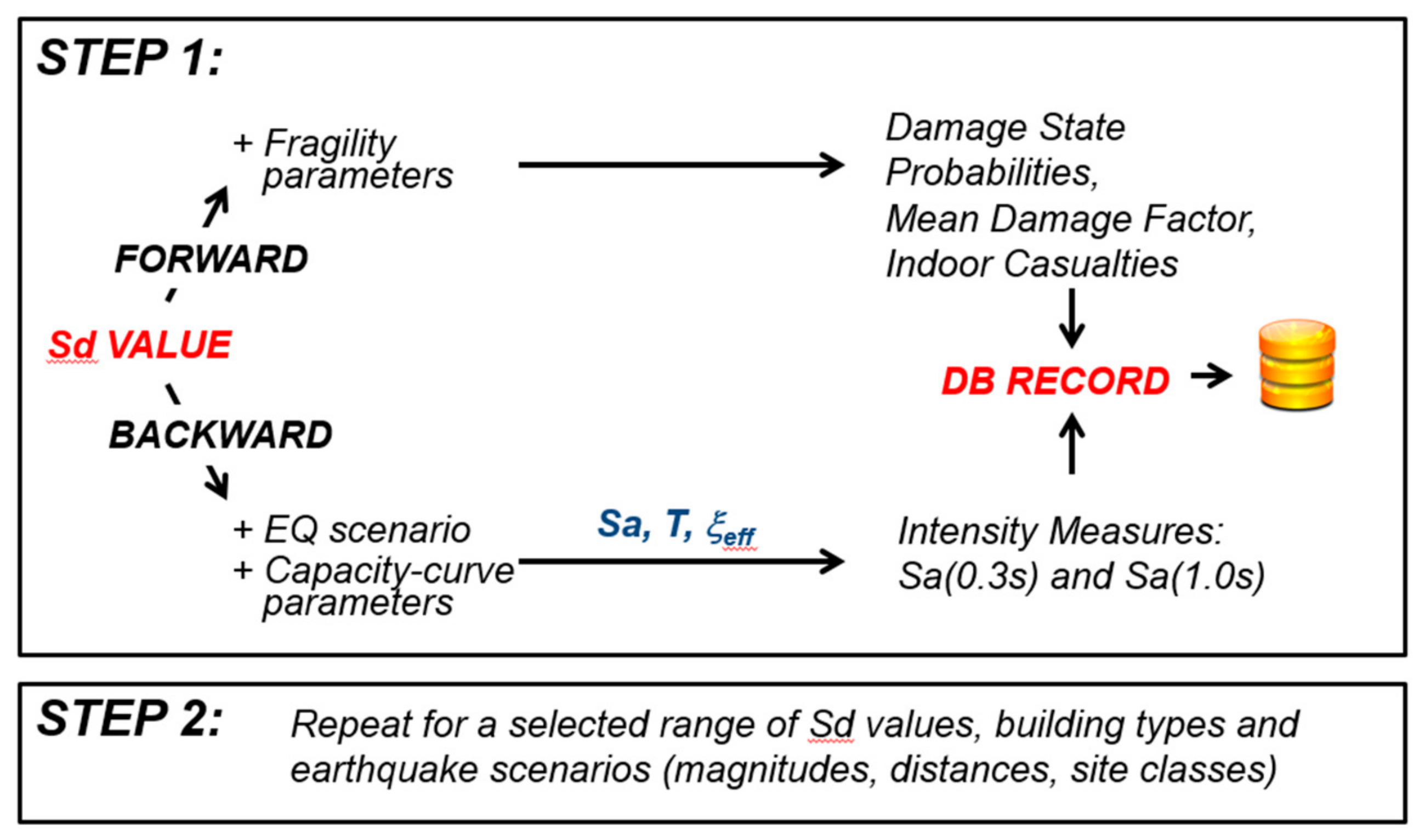
2.1. Background of the Methodology

The seismic risk assessment procedure in ER² includes three major steps: (i) determination of the spatial distribution of the shaking IMs for the earthquake scenario in terms of magnitude, distance and local soil conditions; (ii) inventory of building classes in the study area; and (iii) vulnerability modeling applying seismic hazard-compatible fragility functions. The inventory of the existing buildings in ER² uses the same categories and dynamic parameters as those applied in Hazus-MH [23]. From the structural point of view, there are 16 basic structural types depending on the dominant construction material (wood, steel, concrete, masonry and manufactured housing) and lateral force resisting system (bearing wall, shear wall, frame, etc.). Three general height categories reflect the variation of the fundamental period of building: low: 1–3 storeys, medium: 4–7 storeys, and high-rise: 8 + storeys, for a total of 36 building types as listed in

Table A1. Building types as defined by Hazus-MH [23].

Material	Description/Lateral Force Resisting System	Label	No.	Height Subclasses 1
Wood buildings	Light wood frame single- or multiple-family dwellings of one or more stories in height	W1	1	W1
	Wood frame commercial and industrial buildings with a floor area larger than 5000 square feet	W2	2	W2
Steel buildings	Steel moment frame	S1	3	S1L
			4	S1M
			5	S1H
	Steel braced frame	S2	6	S2L
			7	S2M
			8	S2H
	Steel light frame	S3	9	S3
	Steel frame with cast in place concrete shear walls	S4	10	S4L
			11	S4M
			12	S4H
	Steel frame with unreinforced masonry infill walls	S5	13	S5L
			14	S5M
			15	S5H
Concrete Buildings	Concrete moment frame	C1	16	C1L
			17	C1M
			18	C1H
	Concrete shear walls	C2	19	C2L
			20	C2M
			21	C2H
	Concrete frame with unreinforced masonry infill walls	C3	22	C3L
			23	C3M
			24	C3H
Precast concrete buildings	Precast concrete tilt-up walls	PC1	25	PC1
	Precast concrete frames with concrete shear walls	PC2	26	PC2L
			27	PC2M
			28	PC2H
Reinforced masonry buildings	Reinforced masonry bearing walls with wood or metal deck diaphragms	RM1	29	RM1L
			30	RM1M
	Reinforced masonry bearing walls with precast concrete diaphragms	RM2	31	RM2L
			32	RM2M
			33	RM2H
Unreinforced masonry buildings	Unreinforced masonry bearing walls	URM	34	URML
			35	URMM
Mobil homes	Mobil homes	MH	36	MH

¹ L (low: 1–3 storeys); M (medium: 4–7 storeys); H (high-rise: 8+ storeys).

in Appendix A. The apparent resistance to seismic loads for each building type is assigned with one of the design categories: pre-code, low-code, moderate-code, and high-code, which are functions of the quality of the construction determined by the construction practices, year of construction and regional seismic settings resulting in standard 128 generic building classes.

It has been shown that building classification schemes in Canada and in the US are similar [24,25,26]. It is also known that the building classification can be done differently under different construction and seismic settings. For example, masonry buildings in Europe are separated depending on the structural material (stone, brick, concrete block), floor diaphragm type (flexible wood or rigid concrete) and the quality of material and construction [8,9,16,27,28]. Conducted building inventories in Eastern Canada identified two main types of unreinforced masonry (URM): stone masonry [15] and brick masonry [17] which, as the most frequent ones, were retained for this study. The later matches the description for URM buildings in Hazus-MH, which combines all types of floor diaphragms including wood or cast-in-place concrete floor. This approach is considered reasonable in the context of a regional seismic risk study.

The vulnerability modeling in ER² is inspired by the standard framework for performance-based earthquake engineering [21,29,30]. The method relies on the two ground motion IMs, where the spectral acceleration Sa(0.3s) is generally associated with the dynamic response of stiffer low-rise buildings in the short period range, and Sa(1.0s) reflects the dynamic response of taller, more flexible buildings in the longer period range. Both IMs fully define the simplified 5%-damped ‘input response spectrum’ for a given seismic scenario. The maximal structural response of the considered building class, referred to as the ‘performance point’, is obtained using the CSM [20,31]. The performance point is determined by the intersection between its structural capacity curve and the input response spectrum adjusted for the inelastic structural damping ratio, ξ_eff, associated with cyclic degradation considered through a degradation factor K function of the duration of shaking and the building class, i.e., the demand spectrum [7]. To avoid the time consuming iterative process usually involved in the determination of the performance point, fragility functions in ER² are expressed as explicit functions of the earthquake magnitude and the input IMs [15,21,22]. They provide the probability of a given damage state (none, slight, moderate, extensive, complete) for the building structural and non-structural components, respective economic losses and indoor casualties.

The procedure starts with the assumption of the performance point with respective spectral displacement Sd, spectral acceleration Sa, and effective damping ratio ξ_eff on the intersection of the capacity curve and the demand spectrum. The demand spectrum is then correlated to the standard 5% damped input response spectrum defined with the two structure-independent IMs, Sa(0.3s) and Sa(1.0s), from the seismic scenario. Their values are obtained using the spectral reduction factor relationship proposed by Porter [21]. The equations and related tables were implemented in the ER² computation model [22]. Next, the Sd of the performance point is combined with a set of displacement based fragility functions for the considered building class to obtain the probability of being in each of the five potential damage states. The full set of fragility data was developed based on the Canadian seismic hazard settings. The spectral accelerations were generated for earthquake scenarios using the AA13 ground motion prediction equation (GMPE) currently used in NBCC 2015 [13], whereas the capacity parameters and damage state thresholds were those for the 128 generic building classes as defined in Hazus-MH [23].

The last step consists in correlating the obtained probabilistic damage states to the IM closest to the performance point and computation of the other IM. This allows for a direct evaluation of the expected structural, non-structural and content damage given a ground motion scenario. Based on these probabilities, indoor casualties and economic losses sustained by the building structure and contents are calculated using inventory information on occupancy class, replacement cost and number of occupants and results are stored in a database. The flow chart of the procedure is shown on Figure 1.

2.2. Database of Damage State Probabilities

A database of pre-computed damage estimates for IMs of the magnitude-distance-site condition scenarios was generated for each of the 128 generic building classes by gradually increasing the shaking intensity. The process starts with low IMs yielding response spectral displacement Sd close to zero and the successively for Sd values equally spaced on the logarithmic scale ranging from 10⁻² to 10³ inches (0.025 cm to 2500 cm) until the ultimate point on the capacity curve is attained. The corresponding earthquake scenarios were generated by permutations of four magnitudes (M5, M6, M7, M8), five distances (10, 20, 30, 40 and 60 km) and five site classes (A, B, C, D, E), for a total of 100 earthquake scenarios. The generated vulnerability functions were then tabulated in a database giving performance points, respective probabilistic damage states and associated IMs. The complete database includes three tables created for different GMPEs, two for Eastern North America (ENA) and one for Western North America (WNA) [12,13,14], for a total of 38,400 tests or ≈2 million vulnerability results. Once developed, the database of damage state probabilities conditioned to the input IMs could readily be used for assessing the expected building damage and corresponding economic and social losses for any potential level of seismic shaking (magnitude-distance-site condition scenarios).

2.3. Optimization of Building Inventories

2.3.1. Inventory Scheme with 53 Most Frequent Building Classes

The optimization of near-real time post-earthquake damage computation done by simplifying the earthquake magnitude-distance-site class scenarios considered in the development of the fragility functions and by reducing the building classification scheme is discussed in this section. To reduce the number of building classes, only the 53 most common construction types representing the construction practices in Eastern Canada was retained, while excluding the remaining 75 less frequent building classes from the further analyses (see Table A1).

Table 1. The 53 most frequent building classes.

Material	Description/Lateral Force Resisting System	Label	Height	Code Level
Wood buildings	Light wood frame single- or multiple-family dwellings of one or more stories in height	W1	Low-rise	Pre-code Low-code Medium-code
	Wood frame commercial and industrial buildings with a floor area larger than 5000 square feet	W2	Low-rise	Pre-code Low-code Medium-code
Steel buildings	Steel moment frame	S1	Low-rise Medium-rise High-rise	Pre-code Low-code
	Steel braced frame	S2	Low-rise Medium-rise High-rise	Pre-code Low-code
	Steel light frame	S3	Low-rise	Pre-code Low-code
	Steel frame with cast in place concrete shear walls	S4	Low-rise Medium-rise High-rise	Pre-code Low-code
	Steel frame with unreinforced masonry infill walls	S5	Low-rise Medium-rise High-rise 1	Pre-code Low-code
Concrete Buildings	Concrete moment frame	C1	Low-rise Medium-rise High-rise	Pre-code Low-code
	Concrete shear walls	C2	Low-rise Medium-rise High-rise	Pre-code Low-code
	Concrete frame with unreinforced masonry infill walls	C3	Low-rise Medium-rise High-rise	Pre-code Low-code
Unreinforced masonry buildings	Unreinforced masonry bearing walls	URM	Low-rise Medium-rise	Pre-code Low-code

¹ High-rise pre-code S5 is not considered.

lists the retained building classes defined as combination of material and lateral resisting system: light wood frame structures (W1, W2), steel (S1, S2, S3, S4, S5), concrete (C1, C2, C3), and URM. Depending on the height these buildings can be low-rise (L), medium-rise (M) or high-rise (H) and designed with low-code (l), pre-code (p) or moderate code (m). As a consequence, the comprehensive ER² database of pre-computed IMs and respective damage estimates was significantly reduced based on 75 earthquake scenarios applying the AA13 GMPE [13] for 3 magnitudes (M5, M6, M7); 5 distances (10 km, 20 km, 30 km, 40 km, 60 km); and 5 NEHRP/NBC site classes (A, B, C, D, E). With this, the access to the smaller database was accelerated and the unessential computations for the infrequent building classes were avoided.

2.3.2. Reduced Inventory Scheme with 24 Combined Building Classes

The visual screening of existing buildings and identification of the pertinent building class during the inventory process involves significant uncertainties in particular for a large inventory of buildings. Whereas the year of construction, number of stories, occupancy and footprint area of a given building can be obtained from the information stored in municipal property assessment database, identification of the structural system is more complicated. In many cases, the visual screening is insufficient and the identification of the structural system would require detailed checking and consultation of as built drawings (e.g., concrete shear-wall, concrete frame, etc.). This makes the building inventory relatively uncertain, tedious and time-consuming process. To reduce the epistemic uncertainties, a simplified building classification scheme was introduced next. Regrouping different structural systems into a single combined class does not imply that their seismic behavior would be similar. It provides implicit fragility functions for aggregated damage to a population of buildings only applicable to regional scales and not for a specific building.

Namely, the number of retained 53 building classes was further reduced to 24 combined classes by grouping together building types with similar structural parameters (e.g., construction material, height, design code level) and, what is most important, that are expected to have similar vulnerability to earthquake motion. The latter condition was validated by measuring the differences and spread of the damage state probabilities.

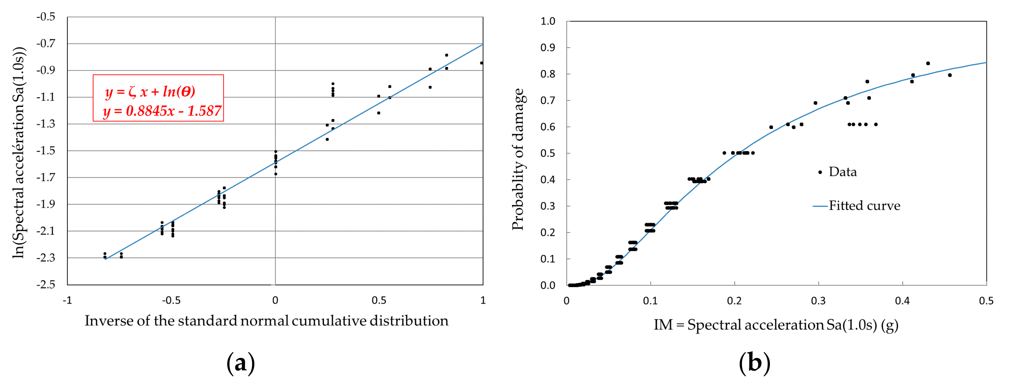
2.4. Fitting Implicit Fragility Curves for Single IM

The next optimization step was the selection of single IM, Sa(1.0s), against which the vulnerability of structural and non-structural components is determined. Two sets of fragility functions were generated for the 53 and then for the 24 building classes by fitting a standard lognormal curve with own median and a standard deviation through a cloud of points representing the probabilities of damage for a given level of the IM (earthquake scenarios as combination of magnitudes/distances/site classes). Each of the data points can be associated with ‘individual scenario’, i.e., one building class and one IM corresponding to one magnitude-distance-site class scenario.

An example of the fitting procedure applied to generate the fragility functions is given in Figure 2 to illustrate the applied methodology. It can be observed in this figure that close but different IMs (scenarios) correspond to the same probability of the considered damage state. Fragility curves developed in this way, referred herein as implicit building fragility functions, are functions of the magnitude and the selected IM only while integrating implicitly the variability in the epicentral distance and site class. Cumulative damage probabilities to reach slight damage were extracted from the global ER² database for low- and medium-code light wood frame building class, W1-l and W1-m. In this example, twenty-five earthquake scenarios were generated for magnitude M6 by permutations of five distances (10, 20, 30, 40 and 60 km) and five NEHRP/NBCC site classes (A, B, C, D, E) scaled in increasing levels of Sa(1.0s). Cumulative probability for the slight damage state is given in terms of Sa(1.0s) as IM. A total of 2550 points, for 50 individual scenarios, are shown in the same graph for W1-l and W1-m and all permutations of magnitudes-distances-site class scenarios. The natural logarithm of the IM is then depicted against the inverse of the standard normal cumulative distribution (Figure 2a). The two parameters a and b of the linear approximation (y = ax + b) on Figure 2a correspond, respectively, to the standard deviation (ζ) and the natural logarithm of the median (ln(θ)) of the lognormal distribution. These parameters obtained from the linear approximation define the implicit fragility function illustrated in Figure 2b.

To improve the fitting accuracy, the median and standard deviation of the implicit fragility curve were used as tuning parameters and were gradually adjusted during the iterative procedure implemented in a Matlab code (MathWorks Inc., Natick, MA, USA).

3. Results

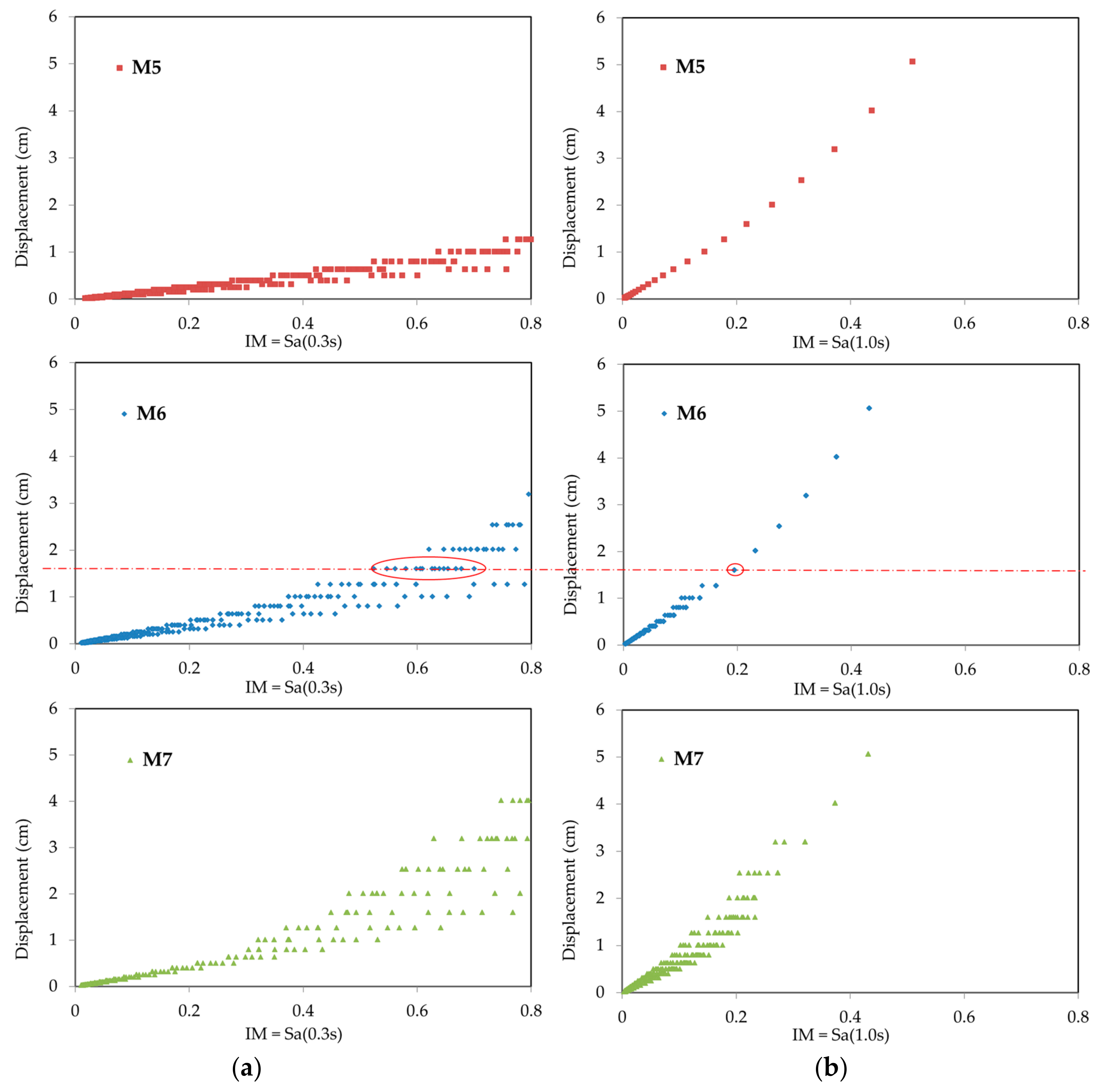
3.1. Selecting Single Intensity Measure

For simplified damage assessment at regional scale, fragility functions are typically conditioned on a single IM such as peak ground acceleration (PGA), peak ground velocity (PGV), spectral acceleration at specific periods (e.g., Sa(0.3s) or Sa(1.0s)). These IMs are referred to as structure-independent, which means that they can be obtained directly from the GMPE without the need to quantify the fundamental period for each building. The most widely used IM for regional risk studies is PGA [6,9]. However, considerable scatter in the damage probabilities were observed when correlating to PGA [28]. In order to reduce the scatter, spectral acceleration near the fundamental period of buildings is recommended such as the Sa(0.3s) for short period and the Sa(1.0s) for intermediate to long building periods. On the other hand, recent studies have shown that even for short period buildings such as URM, the Sa(1.0s) can be the preferred IM since it correlates better with observed damage [32]. Porter [21] indicated that the preferred IM should correlate to the seismic displacement demand, or the location of the performance point on the spectrum, i.e., Sa(0.3s) for the constant acceleration portion and Sa(1.0s) for the constant velocity portion. To the author’s knowledge, literature on comparative studies on the scatter of the seismic demand in correlation to the two IMs for regional scale studies is scarce. Before generating implicit fragility functions, comparative analyses were conducted to determine which IM represents better the seismic scenario in terms of risk assessment and exhibits less scatter to the magnitude-distance-site class scenarios for a given building class. Examples of the displacement demands at the performance point in terms of Sa(0.3s) and Sa(1.0s) for low-rise pre-code URM buildings are given in Figure 3 for the same magnitude (M5, M6, M7), distance (10, 20, 30, 40 and 60 km) and site class (A, B, C, D, E) seismic scenarios extracted from the ER² global database. Each graph on Figure 3 contains 1275 data points.

A given displacement demand can be associated with more than one earthquake scenario, and therefore several possible combinations of values of Sa(0.3s) and Sa(1.0s). For example, considering magnitude M6 it can be observed that a displacement demand of 1.6 cm can be associated with several distance-site class scenarios (data points) identified by Sa(0.3s) in Figure 3a or by Sa(1.0s) in Figure 3b. These scenarios correspond to data points scattered between 0.5 g to 0.7 g when using Sa(0.3s) as IM, and at the same time they correspond to a single value of Sa(1.0s) equal to 0.2g. In general, data points of the considered scenarios show considerably less scatter with Sa(1.0s) when compared to that with Sa(0.3s).

It can also be observed in Figure 3a that when correlated to Sa(0.3s), lower variability of the displacement demand corresponds to low intensity of shaking (Sa(0.3s) < 0.2 g). This is explained by the fact that for low shaking levels, damage to buildings is minimal and the performance point typically intercepts the constant acceleration portion of the input spectrum, making Sa(0.3s) the preferred IM for low intensity of shaking. On the other hand, for higher intensity of shaking there is less variability in the displacement demand when correlated to Sa(1.0s) as shown on Figure 3b. In such cases, buildings are more likely to be damaged and the performance point typically intercepts the constant velocity portion of the input spectrum and corresponds to a building response with effective period larger than the fundamental period due to increased nonlinear behavior, making Sa(1.0s) the better predictor IM for higher intensities of shaking. These observations are valid for all considered building classes. Based on the above observations and in order to simplify the damage assessment procedure, Sa(1.0s) was selected as the single IM used to generate the sets of implicit building fragility functions. The generated fragility functions are only applicable to buildings subjected to a ground motion of a single event. For already damaged buildings subjected to series of aftershocks, special considerations on the damage accumulation should be considered [33,34,35], which is outside the scope of this study.

3.2. Sensitivity of Implicit Fragility Functions to Epicentral Distance and Site Class

Having selected Sa(1.0s) as the intensity measure, a Matlab code was developed to compute the median and standard deviation of the fitted implicit fragility functions for each of the 53 building classes. Only the estimates of the structural damage are discussed herein. Sensitivity analysis was conducted next with a twofold objective: to analyze the potential error of damage probabilities to epicentral distance and site class, and to evaluate the deviation between the best fit implicit fragility function and the data points for M5, M6 and M7 earthquake scenarios (combining all distances and all site classes), for a total of 3975 tests. It was also observed during the fitting process that a better fit was obtained when the range Sa(1.0s) ≥ 0.1 g was considered, i.e., scenarios corresponding to the lower Sa(1.0s) values were ignored. This resulted in negligible additional errors in damage prediction for Sa(1.0s) < 0.1 g (average absolute deviation of less than 3.5%) while significantly improving the approximation for larger values of IM.

For all 53 building classes, for M5 scenarios, the results showed very low scatter to the epicentral distance and site class as data points of the damage probabilities almost coincide for all distance-site classes scenarios. This is also observed for M6 and M7 scenarios for reinforced concrete (C1, C2, C3) and steel building classes (S1, S2, S3, S4, S5). This is illustrated in Figure 4a where the final implicit fragility functions are shown for high-rise low-code steel braced frame (S2H-l), for each structural damage state and for M5, M6 and M7 scenarios, respectively. For URM and wood frame (W1 and W2) buildings, certain dispersion can be observed in data points for damage probabilities for Sa(1.0s) < 0.25 g and Sa(1.0s) > 0.4 g. This is illustrated in Figure 4b where the final implicit fragility functions are shown for low-rise pre-code unreinforced masonry building (URML-p), for each structural damage state and for M5, M6 and M7 scenarios, respectively.

To estimate the margin of error between the implicit fragility function and the data points, the Average Absolute Deviation is calculated for each considered IM value along the curve, and the overall mean was calculated as a single parameter for each fragility function, referred to as MAAD parameter. The MAAD parameter is calculated in terms of damage probability.

Table 2. Building classes with maximum deviation between damage probability data points and implicit fragility function observed for 53 building classes—MAAD parameter (mean of the average absolute deviation).

Earthquake Scenarios	Damage State	Maximum MAAD	Building Class
M5, all distances and all site classes	Slight	2.91%	S3-p
	Moderate	1.77%	S3-p
	Extensive	0.78%	S3-p
	Complete	0.28%	S3-p
M6, all distances and all site classes	Slight	3.17%	S3-p
	Moderate	1.96%	S3-p
	Extensive	0.86%	S3-p
	Complete	0.33%	S3-p
M7, all distances and all site classes	Slight	3.43%	URML-p
	Moderate	1.96%	S3-p
	Extensive	0.86%	S3-p
	Complete	0.33%	S3-p

gives a summary of building classes with maximum deviation between damage probability data points and implicit fragility functions obtained with MAAD for all scenarios and damage states.

Table 2 indicates that for all 53 buildings classes the maximum MAAD parameter is below 1% for extensive and complete damage states and below 2% for moderate damage state. For slight damage state, the MAAD parameter remains below 3.0% for most building classes while it reaches 3.2% for S3-p for M6 scenarios and 3.5% for URML-p for M7 scenarios. The MAAD parameter provides an absolute value of the deviation regardless if it represents an overestimation or underestimation. The degree of over- or underestimation of the implicit fragility functions depends on the value of the IM and the damage state. For example, in Figure 4b, the URML-p fragility functions for slight and moderate damage underestimate the damage up to Sa(1.0s) = 0.05 g. On the other hand, for Sa(1.0s) ranging from 0.05 g to 0.25 g, they overestimate the damage probability. For Sa(1.0s) higher than 0.25 g, the implicit fragility functions nearly coincide with the discrete damage state probability points.

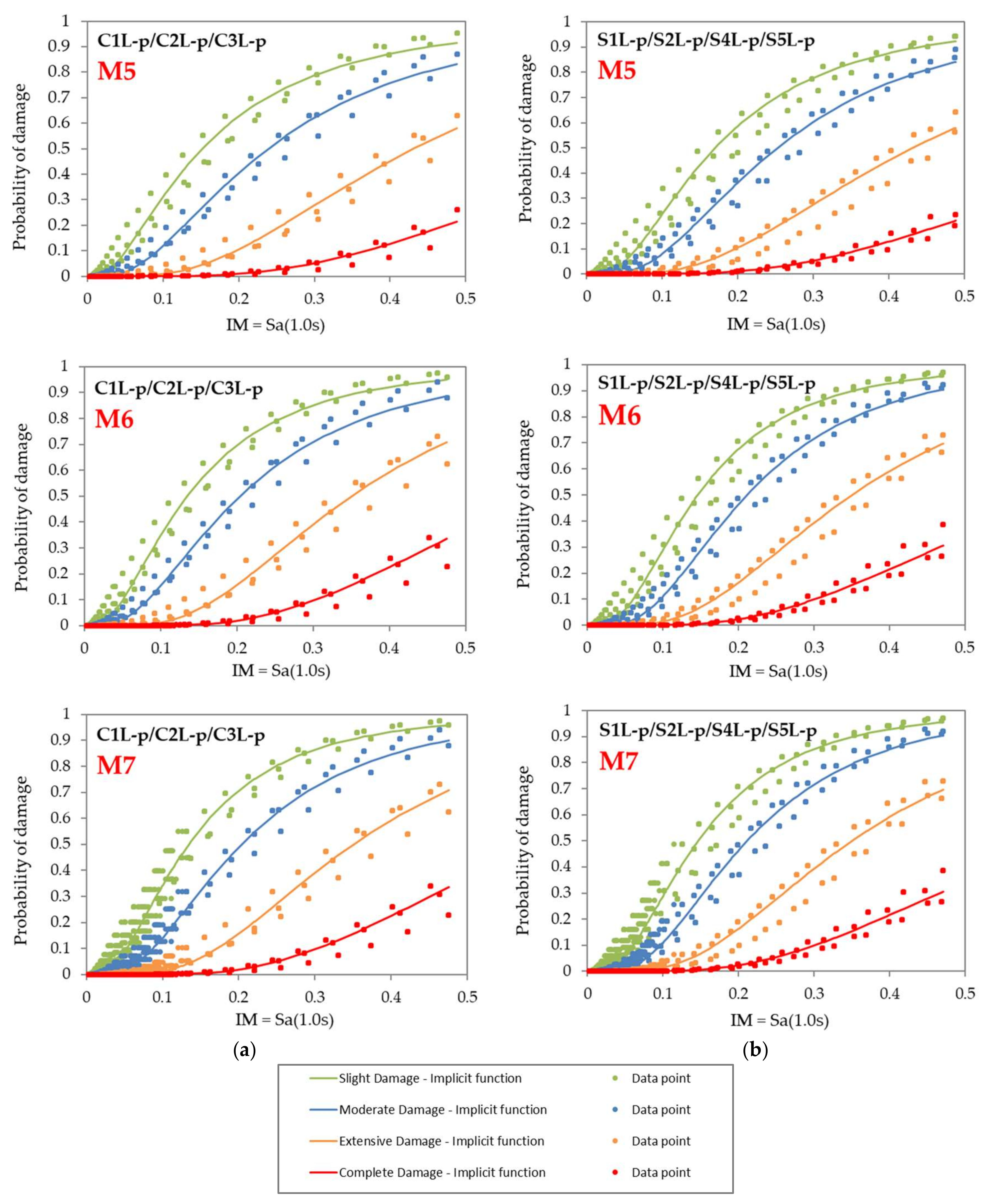
3.3. Implicit Fragility Fucntions for Simplified Building Classification

Considering the epistemic uncertainty in the inventory procedure resulting from the difficulties in the assignment of the appropriate building class, the use of a simplified building classification is judged more suitable in the context of rapid risk assessment immediately following a strong earthquake event. The following criteria were adopted to reduce the number of building classes from 53 (Table 1) to 24:

• group building classes with similar material, same height range and same code level;
• group building classes for which the lateral force resisting system is difficult to identify with visual screening;
• keep separate the building classes of the same structural system that can be easily identified knowing the height, year of construction or occupancy, information available in municipal property assessment database.

Table 3. Proposed simplified building classes.

Material	Description/Lateral Force Resisting System	Label	Height	Code Level 1
Wood buildings	Light wood frame single- or multiple-family dwellings of one or more stories in height	W1	Low-rise	Pre-code Low-code Medium-code
	Wood frame commercial and industrial buildings with a floor area larger than 5000 square feet	W2	Low-rise	Pre-code Low-code Medium-code
Steel buildings	Steel moment frame (S1), Steel braced frame (S2), Steel frame with cast in place concrete shear walls (S4), Steel frame with unreinforced masonry infill walls (S5)	S	Low-rise Medium-rise High-rise	Pre-code Low-code
	Steel light frame	S3	Low-rise	Pre-code Low-code
Concrete Buildings	Concrete moment frame (C1), Concrete shear walls (C2), Concrete frame with unreinforced masonry infill walls (C3)	C	Low-rise Medium-rise High-rise	Pre-code Low-code
Unreinforced masonry buildings	Unreinforced masonry bearing walls	URM	Low-rise Medium-rise	Pre-code Low-code

¹ Design code level as defined in Section 2.1.

presents the proposed simplified building classification, where the combination of the height and design code level produces 24 classes compared to the most frequent 53 building classes given in Table 1. Building descriptions and definition of the lateral force resisting systems used in Table 3 are according to the visual screening procedure described in [36].

Implicit fragility functions are provided for the concrete building class (C) regrouping all lateral force resisting systems (C1, C2 and C3) and for steel building class (S) regrouping most of the lateral force resisting systems (S1, S2, S4 and S5). The lateral force resisting system of these buildings is generally hidden behind the façade and the internal walls, making difficult the distinction between frame, wall or braced frame buildings. The authors acknowledge that grouping these different structural systems under a single building category does not imply that the seismic behavior of, for example, concrete frame building would be similar to that of a shear wall building. Knowing that the time necessary for the computation was more important factor than the accuracy of the damage estimates, the objective was to provide implicit fragility functions for damage of aggregated population of concrete buildings with different lateral load resisting systems that are only applicable to rapid urban and regional scale seismic risk studies.

Implicit fragility functions are provided for the following separate building classes which can be easily identified from visual screening or their occupancy:

• S3: these light frames low rise are mostly used for agricultural structures, industrial factories, and warehouses and can be easily identified from occupancy and height.
• W1 and W2: these wood building classes can be identified by the occupancy as W1 are light wood frame single- or multiple-family dwellings of one or more stories in height and W2 are wood frame commercial and industrial buildings with a floor area larger than 5000 square feet.
• URM: unreinforced masonry building class can be easily identified by visual screening.

Figure 5 shows data points of damage probabilities for magnitudes M5, M6 and M7 and four damage states for two groups of specific building classes, as defined in Table 1: low-rise pre-code C1, C2 and C3 (Figure 5a) and low-rise pre-code S1, S2, S4 and S5 (Figure 5b). It also shows the corresponding implicit fragility functions for the simplified reinforced concrete building class C and simplified steel building class S.

Table 4. Building groups with maximum deviation between damage probability data points and implicit fragility function observed for 24 building classes—MAAD parameter.

Earthquake Scenarios	Damage State	Maximum MAAD	Building Group
M5 all distances and all site classes	Slight	3.58%	C1L-l + C2L-l + C3L-l
	Moderate	2.30%	S1L-l + S2L-l+ S4L-l + S5L-l
	Extensive	1.71%	C1L-l + C2L-l + C3L-l
	Complete	0.62%	C1H-p + C2H-p + C3H-p
M6 all distances and all site classes	Slight	3.33%	C1L-p + C2L-p + C3L-p
	Moderate	2.37%	C1H-p + C2H-p + C3H-p
	Extensive	1.88%	C1H-p + C2H-p + C3H-p
	Complete	0.93%	C1H-p + C2H-p + C3H-p
M7 all distances and all site classes	Slight	3.12%	C1L-p + C2L-p + C3L-p
	Moderate	2.37%	C1H-p + C2H-p + C3H-p
	Extensive	1.88%	C1H-p + C2H-p + C3H-p
	Complete	0.93%	C1H-p + C2H-p + C3H-p

gives a summary of the building groups with maximum deviation between damage probability data points and implicit fragility functions obtained with MAAD. For reinforced concrete building class C and simplified steel building class S, maximum values of MAAD are below 2% for extensive and complete damage states and below 2.5% for moderate damage state. For slight damage state, MAAD parameter remains below 3.6%.

Figure 5 shows almost no difference between the damage probabilities and the implicit fragility functions conditioned on magnitude M6 or M7. This similarity is related to the simplification inherent to the capacity spectrum method. The effect of magnitude is mainly considered through the idealized degradation factor K which reduces the energy dissipation capacity according to the strong motion duration (short, medium, long). In the CSM, the magnitude M < 5.5 is considered to generates short duration, 5.5 < M < 7.5 range generates medium duration and M > 7.5 generates long duration. Therefore, degradation factors are the same for M6 and M7 resulting in similar displacement responses and damage probabilities provided that the IMs are the same. Therefore, the implicit fragility functions in this study are presented in terms of the magnitude ranges M < 5.5 and 5.5 < M < 7.5. The median and standard deviation for these implicit damage fragility functions for simplified reinforced concrete building class C and simplified steel building class S are given in

Table A2. Median and standard deviation for simplified reinforced concrete (C) and simplified steel buildings (S) for short strong motion duration (M ≤ 5.5).

Building Class	Slight Damage		Moderate Damage		Extensive Damage		Complete Damage
	Median	St. Dev.	Median	St. Dev.	Median	St. Dev.	Median	St. Dev.
C1L_p + C2L_p + C3L_p	0.15	0.85	0.24	0.74	0.43	0.61	0.77	0.58
C1M_p + C2M_p + C3M_p	0.17	0.68	0.27	0.63	0.50	0.58	0.90	0.61
C1H_p + C2H_p + C3H_p	0.13	0.69	0.21	0.68	0.48	0.80	0.96	0.79
C1L_l + C2L_l + C3L_l	0.21	0.82	0.33	0.73	0.59	0.57	1.07	0.61
C1M_l + C2M_l + C3M_l	0.23	0.69	0.35	0.63	0.67	0.59	1.40	0.72
C1H_l + C2H_l + C3H_l	0.17	0.67	0.29	0.72	0.60	0.74	1.33	0.82
S1L_p + S2L_p + S4L_p + S5L_p	0.17	0.74	0.25	0.66	0.43	0.61	0.79	0.59
S1M_p + S2M_p + S4M_P + S5M_p	0.17	0.66	0.26	0.60	0.50	0.66	0.97	0.70
S1H_p + S2H_p + S4H_p	0.14	0.73	0.22	0.70	0.54	0.86	1.29	0.86
S1L_l + S2L_l + S4L_l + S5L_l	0.23	0.74	0.32	0.67	0.52	0.53	0.89	0.53
S1M_l + S2M_l + S4M_l + S5M_l	0.24	0.65	0.34	0.63	0.60	0.56	1.44	0.79
S1H_l + S2H_l + S4H_l + S5H_l	0.18	0.72	0.29	0.70	0.66	0.78	1.37	0.84

and

Table A3. Median and standard deviation for simplified reinforced concrete (C) and simplified steel buildings (S) for medium strong motion duration (5.5 < M ≤ 7.5).

Building Class	Slight Damage		Moderate Damage		Extensive Damage		Complete Damage
	Median	St. Dev.	Median	St. Dev.	Median	St. Dev.	Median	St. Dev.
C1L_p + C2L_p + C3L_p	0.13	0.77	0.20	0.70	0.35	0.56	0.60	0.53
C1M_p + C2M_p + C3M_p	0.15	0.64	0.23	0.60	0.41	0.53	0.73	0.59
C1H_p + C2H_p + C3H_p	0.12	0.63	0.19	0.62	0.37	0.65	0.73	0.68
C1L_l + C2L_l + C3L_l	0.18	0.71	0.26	0.66	0.44	0.53	0.74	0.53
C1M_l + C2M_l + C3M_l	0.19	0.60	0.29	0.56	0.51	0.53	1.09	0.69
C1H_l + C2H_l + C3H_l	0.16	0.60	0.25	0.67	0.51	0.74	1.06	0.78
S1L_p + S2L_p + S4L_p + S5L_p	0.15	0.69	0.21	0.61	0.35	0.57	0.63	0.58
S1M_p + S2M_p + S4M_P + S5M_p	0.16	0.58	0.22	0.56	0.39	0.57	0.68	0.61
S1H_p + S2H_p + S4H_p	0.13	0.68	0.20	0.63	0.41	0.68	0.77	0.64
S1L_l + S2L_l + S4L_l + S5L_l	0.18	0.65	0.27	0.59	0.42	0.49	0.79	0.57
S1M_l + S2M_l + S4M_l + S5M_l	0.19	0.58	0.28	0.56	0.49	0.54	0.81	0.56
S1H_l + S2H_l + S4H_l + S5H_l	0.17	0.63	0.26	0.65	0.52	0.67	1.11	0.77

in the Appendix.

Table A4. Median and standard deviation for buildings classes for short strong motion duration (M ≤ 5.5).

Building Class	Slight Damage		Moderate Damage		Extensive Damage		Complete Damage
	Median	St. Dev.	Median	St. Dev.	Median	St. Dev.	Median	St. Dev.
S3-l	0.14	0.85	0.21	0.73	0.40	0.65	0.70	0.50
S3-p	0.11	0.95	0.17	0.79	0.32	0.72	0.59	0.53
URML-l	0.14	0.97	0.27	0.96	0.60	0.95	1.42	0.96
URML-p	0.11	1.15	0.22	1.12	0.46	1.00	1.08	1.02
URMM-l	0.16	0.89	0.28	0.75	0.56	0.62	1.21	0.71
URMM-p	0.12	0.95	0.22	0.79	0.44	0.64	0.81	0.60
W1-l	0.21	0.95	0.53	1.00	1.68	1.04	4.24	1.01
W1-m	0.21	0.93	0.59	0.96	2.06	0.99	5.69	1.16
W1-p	0.16	1.00	0.38	0.98	1.08	1.00	2.20	0.93
W2-l	0.27	0.83	0.55	0.72	1.26	0.66	2.43	0.74
W2-m	0.33	0.92	0.84	0.99	2.36	0.92	4.67	0.83
W2-p	0.20	0.84	0.40	0.74	0.89	0.64	1.53	0.66

and

Table A5. Median and standard deviation for building classes for medium strong motion duration (5.5 < M ≤ 7.5).

Building Class	Slight Damage		Moderate Damage		Extensive Damage		Complete Damage
	Median	St. Dev.	Median	St. Dev.	Median	St. Dev.	Median	St. Dev.
S3-l	0.13	0.76	0.18	0.72	0.33	0.61	0.60	0.51
S3-p	0.10	0.84	0.14	0.74	0.26	0.64	0.48	0.54
URML-l	0.13	0.92	0.24	0.87	0.50	0.86	1.01	0.81
URML-p	0.10	1.05	0.19	0.98	0.38	0.87	0.80	0.90
URMM-l	0.14	0.77	0.25	0.69	0.48	0.58	0.82	0.58
URMM-p	0.11	0.87	0.20	0.72	0.36	0.55	0.65	0.56
W1-l	0.19	0.89	0.44	0.88	1.21	0.92	2.39	0.83
W1-m	0.21	0.87	0.54	0.90	1.73	0.93	4.49	1.09
W1-p	0.16	0.97	0.34	0.89	0.82	0.85	1.91	0.90
W2-l	0.22	0.75	0.43	0.65	0.91	0.60	1.51	0.62
W2-m	0.28	0.78	0.62	0.84	1.68	0.84	2.75	0.70
W2-p	0.18	0.76	0.34	0.66	0.68	0.57	1.26	0.63

present the median and standard deviation for the implicit fragility functions for specific building classes S3, W1, W2 and URM.

4. Discussion

The implicit fragility functions presented in this paper were developed for implementation in ER², a user-friendly regional and urban scale seismic risk assessment tool. The main objective was to accelerate the computation process for near real-time risk analyses in minutes following a major earthquake event. The final functions were generated for a reduced number of combined building classes, 24 instead of 53 building classes common for construction practice in Eastern Canada. The earthquake scenarios used in their development were based on magnitude (M5, M6 and M7) and incorporate five epicentral distances (10, 20, 30, 40 and 60 km) and five NEHRP/NBC site classes (A, B, C, D, E). In terms of the nonlinear structural response and the respective effective damping, the implicit fragility functions for the combined 24 buildings classification scheme were developed for short strong motion duration, magnitude range of M < 5.5, and for medium duration, magnitude range of 5.5 < M < 7.5. To avoid any computational incongruity by applying such wide magnitude ranges, it is recommended to develop continuous correlation between the degradation factor and the magnitude. Such correlation would replace the current discrete degradation factors defined in terms of earthquake duration conditioned on the magnitude.

Instead of the standard approach using two IMs the use of a single IM, Sa(1.0s), is recommended as it provides a simplified approach for damage estimation with satisfactory accuracy. In the presented analyses, both the displacement demand and the corresponding damage probabilities exhibited less scattered when correlated to Sa(1.0s) compared to Sa(0.3s). In terms of damage estimates, the range of the shaking intensity of interest was 0.1 g ≤ Sa(1.0s) ≤ 0.5 g. The implicit fragility functions are lognormal curves representing earthquake scenarios in terms of magnitude and Sa(1.0s) which incorporates the variation in distance and site class. The margin of error between the proposed implicit fragility function and the damage probabilities data points is estimated from the MAAD. This parameter provides an absolute value of the deviation and the degree of over- or underestimation of the implicit fragility functions depends on the value of the IM and the damage state. The maximum value of this parameter is less than 3.5% for slight damage, 2% for moderate damage and as low as 1% for extensive and complete damages. This is acceptable in the context of rapid risk assessment using earthquake scenarios.

A simplified building classification combining together the reinforced concrete building classes and the steel building classes (except S3) was proposed to reduce effort in producing inventories and computing damages. Regrouping different structural systems does not imply that their seismic behavior would be similar. It provides implicit fragility functions for aggregated damage to a population of buildings with different lateral load resisting systems that are only applicable to regional scale risk studies and not for a specific building. The margin of error between the proposed implicit fragility function for the simplified building classes and damage probabilities data points for the specific building classes is estimated from the MAAD. The maximum value of this parameter is less than 3.6% for slight damage, 2.5% for moderate damage and as low as 3% for extensive and complete damages. This deviation is slightly higher than the one obtained using the implicit fragility functions for specific building classes and is acceptable in the context of rapid risk assessment using simplified building classification and earthquake scenarios. It is believed that the errors generated in this way are lower or in the same order of magnitude as are the uncertainties generated during the inventory of the building structural parameters. Hence, using these implicit functions implies accepting an additional degree of uncertainties in damage prediction to the benefit of simplifying the inventory process and increasing efficiency and reduced computation effort needed for rapid risk assessment.

References

1. GEM (Global Earthquake Model). Openquake Platform. Pavia, Italy. Available online: https://github.com/gem/oq-platform (accessed on 9 November 2017).
2. NORSAR. Risk Analysis Software—The SELENA-RISe Open Risk Package. Kjeller, Norway. Available online: selena.sourceforge.net (accessed on 8 January 2018).
3. FEMA-NIBS. HAZUS-MH 2.1: Multi-Hazard Loss Estimation Methodology Earthquake Model; User Manual; Federal Emergency Management Agency, National Institute of Building Science: Washington, DC, USA, 2012; 863p. [Google Scholar]
4. GFDRR (Global Facility for Disaster Reduction and Recovery). Understanding Risk—Review of Open Source and Open Access Software Packages Available to Quantify Risk from Natural Hazards; International Bank for Reconstruction and Development/International Development Association of The World Bank: Washington, DC, USA, 2014; 67p. [Google Scholar]
5. Wald, D.J.; Jaiswal, K.S.; Marano, K.D.; Bausch, D.B.; Hearne, M.G. PAGER—Rapid Assessment of an Earthquake’s Impact; Fact Sheet 2010–3036; U.S. Geological Survey: Reston, VA, USA, 2011; 4p. [Google Scholar]
6. Coburn, A.W.; Spence, R.J.S. Earthquake Protection, 2nd ed.; John Wiley & Sons: Chichester, UK, 2002. [Google Scholar]
7. Kircher, C.A.; Nassar, A.A.; Kustu, O.; Holmes, W.T. Development of building damage functions for earthquake loss estimation. Earthq. Spectra 1997, 13, 663–682. [Google Scholar] [CrossRef]
8. Mouroux, P.; Le Brun, B. Presentation of RISK-UE project. Bull. Earthq. Eng. 2006, 4, 323–339. [Google Scholar] [CrossRef]
9. Rota, M.; Penna, A.; Strobbia, C.L. Processing Italian damage data to derive typological fragility curves. Soil Dyn. Earthq. Eng. 2008, 28, 933–947. [Google Scholar] [CrossRef]
10. Nastev, N.; Nollet, M.-J.; Abo El Ezz, A.; Smirnoff, A.; Ploeger, S.K.; McGrath, H.; Sawada, M.; Stefanakis, E.; Parent, M. Methods and tools for natural hazard risk analysis in Eastern Canada—Use of knowledge to understand vulnerability and implement mitigation measures. ASCE Nat. Hazards Rev. 2015, 18, B4015002. [Google Scholar] [CrossRef]
11. NRC (National Research Council). National Building Code of Canada 2015; Associate Committee on the National Building Code, National Research Council: Ottawa, ON, Canada, 2017. [Google Scholar]
12. Atkinson, G.M.; Boore, D.M. Earthquake ground-motion prediction equations for eastern North America. Bull. Seismol. Soc. Am. 2006, 96, 2181–2205. [Google Scholar] [CrossRef]
13. Atkinson, G.M.; Adams, J. Ground motion prediction equations for application to the 2015 Canadian national seismic hazard maps. Can. J. Civ. Eng. 2013, 40, 988–998. [Google Scholar] [CrossRef]
14. Boore, D.M.; Joyner, W.B.; Fumal, T.E. Equations for estimating horizontal response spectra and peak acceleration from Western North American earthquakes: A summary of recent work. Seismol. Res. Lett. 1997, 68, 128–153. [Google Scholar] [CrossRef]
15. Abo El Ezz, A.; Nollet, M.-J.; Nastev, M. Seismic fragility assessment of low-rise stone masonry buildings. Earthq. Eng. Eng. Vib. 2013, 12, 87–97. [Google Scholar] [CrossRef]
16. Lagomarsino, S.; Giovinazzi, S. Macroseismic and mechanical models for the vulnerability and damage assessment of current buildings. Bull. Earthq. Eng. 2006, 4, 415–443. [Google Scholar] [CrossRef]
17. Karbassi, A.; Nollet, M.J. Performance-based seismic vulnerability evaluation of masonry buildings using Applied Element Method in a nonlinear dynamic-based analytical procedure. Earthq. Spectra 2013, 29, 399–426. [Google Scholar] [CrossRef]
18. Freeman, S.A. The Capacity Spectrum Method as a Tool for Seismic Design. In Proceedings of the 11th European Conference on Earthquake Engineering, Paris, France, 6–11 September 1998. [Google Scholar]
19. Freeman, S.A. Review of the development of the capacity spectrum method. ISET J. Earthq. Technol. 2004, 41, 1–13. [Google Scholar]
20. Mahaney, A.; Paret, T.F.; Kehoe, B.E.; Freeman, S.A. The Capacity Spectrum Method for Evaluating Structural Response during the Loma Prieta Earthquake. In Proceedings of the 1993 United States National Earthquake Conference, Memphis, TN, USA, 2–5 May 1993; Volume 2, pp. 501–510. [Google Scholar]
21. Porter, K.A. Cracking an open safe: HAZUS vulnerability functions in terms of structure-independent spectral acceleration. Earthq. Spectra 2009, 25, 361–378. [Google Scholar] [CrossRef]
22. Abo El Ezz, A.; Nollet, M.-J.; Nastev, M. Methodology for Rapid Assessment of Seismic Damage to Buildings in Canadian Settings; Open File 7450; Geological Survey of Canada: Ottawa, ON, Canada, 2014; 41p. [Google Scholar]
23. FEMA-NIBS. HAZUS-MH 2.1: Multi-Hazard Loss Estimation Methodology Earthquake Model; Technical Manual; Federal Emergency Management Agency, National Institute of Building Science: Washington, DC, USA, 2012; 718p. [Google Scholar]
24. NRC. Manual for Screening of Buildings for Seismic Investigation; Institute for Research in Construction, National Research Council: Ottawa, ON, Canada, 1992. [Google Scholar]
25. Ventura, C.E.; Finn, W.L.; Onur, T.; Blanquera, A.; Rezai, M. Regional seismic risk in British Columbia—classification of buildings and development of damage probability functions. Can. J. Civil. Eng. 2005, 32, 372–387. [Google Scholar] [CrossRef]
26. Nollet, M.J.; Désilets, C.; Abo-El-Ezz, A.; Nastev, M. Approche Méthodologique D’inventaire de Bâtiments Pour les Études de Risque Sismique en Milieu Urbain: Ville de Québec, Arrondissement La Cité-Limoilou; Open File 7260; Geological Survey of Canada: Ottawa, ON, Canada, 2013; 93p. [Google Scholar]
27. Uva, G.; Sanjust, C.A.; Casolo, S.; Mezzina, M. ANTAEUS Project for the Regional Vulnerability Assessment of the Current Building Stock in Historical Centers. Int. J. Arch. Heritage 2016, 10, 20–43. [Google Scholar] [CrossRef]
28. Rossetto, T.; Elnashai, A. Derivation of vulnerability functions for European-type RC structures based on observational data. Eng. Struct. 2003, 25, 1241–1263. [Google Scholar] [CrossRef]
29. Moehle, J.; Deierlein, G.G. A framework methodology for performance-based earthquake engineering. In Proceedings of the 13th World Conference on Earthquake Engineering, Vancouver, BC, Canada, 1–6 August 2004. [Google Scholar]
30. Kircher, C.A.; Whitman, R.; Holmes, W.T. Hazus earthquake loss estimation methods. Nat. Hazards Rev. 2006, 7, 45–59. [Google Scholar] [CrossRef]
31. ATC. Seismic Evaluation and Retrofit of Concrete Buildings: ATC-40; Applied Technology Council: Redwood City, CA, USA, 1996. [Google Scholar]
32. Paxton, B.; Elwood, K.J.; Ingham, J.M. Empirical Damage Relationships and Benefit-Cost Analysis for the Seismic Retrofit of URM Buildings. Earthq. Spectra 2017, 33, 1053–1074. [Google Scholar] [CrossRef]
33. Di Sarno, L. Effects of multiple earthquakes on inelastic structural response. Eng. Struct. 2013, 56, 673–681. [Google Scholar] [CrossRef]
34. Goda, K.; Taylor, C.A. Effects of aftershocks on peak ductility demand due to strong ground motion records from shallow crustal earthquakes. Earthq. Eng. Struct. Dyn. 2012, 41, 2311–2330. [Google Scholar] [CrossRef]
35. Li, Q.; Ellingwood, B.R. Performance evaluation and damage assessment of steel frame buildings under main shock-aftershock earthquake sequences. Earthq. Eng. Struct. Dyn. 2007, 36, 405–427. [Google Scholar] [CrossRef]
36. Applied Technology Council (ATC). Rapid Visual Screening of Buildings for Potential Seismic Hazards: A Handbook (FEMA P-154), 3rd ed.; Applied Technology Council: Redwood City, CA, USA, 2015. [Google Scholar]
Figure 1. Flow chart of the development of ER2. Sd: spectral displacement; DB: data base; Sa: spectral acceleration; T: natural period; ξeff: effective damping ratio.
Geosciences 08 00016 g001
Figure 2. Fitting procedure for implicit fragility function for light wood frame building classes W1-l and W1-m experiencing slight damage for the magnitude M6: (a) Linear approximation; (b) Curve fitting.
Geosciences 08 00016 g002
Figure 3. Variation of the displacement demand at the performance point for low-rise pre-code unreinforced masonry building (URML-p) for M5, M6 and M7 and all distances and site classes applying (a) Sa(0.3s) as intensity measure and (b) Sa(1.0s) as intensity measure.
Geosciences 08 00016 g003
Figure 4. Implicit fragility functions for magnitudes M5, M6 and M7: (a) Steel braced frame (S2H-l); (b) Unreinforced masonry (URML-p). Continuous lines are relative to the building classes given in Table 3.
Geosciences 08 00016 g004
Figure 5. Implicit fragility functions for magnitudes M5, M6 and M7: (a) Reinforced concrete building class C (C1 + C2 + C3); (b) Steel building class S (S1 + S2 + S4 + S5). Continuous lines are relative to the building classes given in Table 3.
Geosciences 08 00016 g005