A Bathymetry- and Reflectivity-Based Approach for Seafloor Segmentation


Center for Coastal and Ocean Mapping/National Oceanic and Atmospheric Administration (NOAA) Joint Hydrographic Center, University of New Hampshire, Durham, NH 03824, USA
*
Author to whom correspondence should be addressed.
Geosciences 2018, 8(1), 14; https://doi.org/10.3390/geosciences8010014
Submission received: 13 November 2017
/
Revised: 29 December 2017
/
Accepted: 5 January 2018
/
Published: 8 January 2018
(This article belongs to the Special Issue Marine Geomorphometry)
Abstract
:A robust and flexible technique to segment seafloor acoustic mapping data by analyzing co-located bathymetric digital elevation models and acoustic backscatter mosaics is presented. The algorithm first uses principles of topographic openness, pattern recognition, and texture classification to identify geomorphic elements of the seafloor or “area kernels”, and then derives the final seafloor segmentation by merging or splitting the kernels based on principles of similarity and multi-modality. The output is a collection of homogeneous, non-overlapping seafloor segments of consistent morphology and acoustic backscatter texture. Each labeled segment is enriched by a list of derived, physically-meaningful attributes that can be used for subsequent task-specific analysis.
1. Introduction
Numerous studies have described approaches to seafloor segmentation and classification using acoustic backscatter data from multibeam sonar [1,2,3,4,5,6,7,8,9] or, alternatively, seafloor bathymetry [10,11,12,13,14,15]. However, there are few studies that have offered general methods for using a machine-focused approach to combine and use the information found in co-located bathymetric digital elevation models (DEMs) and acoustic mosaics [16,17,18,19,20,21,22]. Modern multibeam sonars and processing software now typically produce geo-located bathymetry and backscatter mosaic products, thus offering the opportunity to treat both data sets together [21,23]. This paper explores a methodology to combine both bathymetry and backscatter data to automatically segment the seafloor.
The proposed method attempts to mimic the approach taken by a skilled analyst assuming that, when called upon to manually segment a seafloor area, the analyst initially evaluates the context surrounding the area and attempts to take full advantage of both bathymetric and reflectivity products rather than focusing on small-scale geomorphometric variability (e.g., local rugosity). The result is a bathymetry- and reflectivity-based estimator for seafloor segmentation (BRESS) that mimics the positive aspects of the segmentation process as performed by a skilled analyst (e.g., the use of context and multiple inputs) but avoids the inherent deficiencies (subjectivity, processing time, lack of reproducibility). The initial phase of the algorithm performs a segmentation of the DEM surface through the identification of its seafloor “geoform” elements (i.e., contiguous regions of similar morphology, e.g., valleys or edges). These elements represent “area kernels” (regions of consistent morphological type) whose backscatter is then analyzed to derive final seafloor segments by merging or splitting the kernels based on the principles of similarity and multi-modality. The output of BRESS is a collection of homogeneous, non-overlapping seafloor segments. Each labeled segment is enriched by a list of derived, physically-meaningful attributes that can be used for task-specific analysis (e.g., habitat mapping, backscatter model inversion, or change detection).
2. Methods
2.1. Area Kernels Based on Landform Classification
The BRESS algorithm starts by performing a preliminary bathymetry-derived segmentation, that is, a segmentation of the DEM surface through the identification of its seafloor geomorphological (geoform) elements. From the perspective of the final task of the algorithm (a collection of homogeneous, non-overlapping seafloor segments based on both morphology and backscatter), this preliminary step usually provides a general over-segmentation of the area (i.e., a homogenous area is split into more than one segment), although localized cases of under-segmentation (a single segment covers a non-homogenous area) are also possible since only the bathymetry is analyzed in the first step.
Common methods to segment the seafloor into geoform elements use differential geometry and geo-morphometric proxies that are derived locally from the DEM by calculating a variable combination of first and second derivatives [24]. These methods offer several approaches for how the geo-morphometric variables are used (mainly, cell-based or object-based), with respect to the selected units of classification (landforms, landform elements, and physiographic units), and the adopted classifier (based on expert knowledge or driven by a machine learning algorithm) [25,26]. However, well-known limitations (particularly the sensitivity to the selected scale) of these methods have impact on the stability of the overall segmentation algorithm [27,28,29]. Due to this scale-dependent limitation, we have taken a different approach that uses the principles of topographic openness, pattern recognition and texture classification to create ‘area kernels’ (regions of consistent morphological type), evolving this approach from the innovative concepts introduced by [30,31].
To derive geoform elements, we have adapted the concepts of Local Ternary Pattern (LTP) [32] and texton [33] to trigger the preliminary bathymetry-derived segmentation. In image processing, the LTP represents an evolution of the Local Binary Pattern (LBP) texture descriptor introduced by [34]. LBP labels the pixels of an image by thresholding the neighborhood of each pixel and characterizing it with a binary indicator (i.e., a “+” or a “-” that describes the relative value of the pixel with respect to its neighborhood). Despite its simplicity, LBP has been applied successfully to tasks such as texture classification, face recognition, and background modeling [32]. LTP adds a third (neutral) level to the original two possible LBP levels of contrast variation against the central cell. Thus, each direction of evaluation of LTP has three possible states: “+”, “0”, and “-”.
Together with LTP, the BRESS algorithm borrows concepts from texton theory. This theory proposes a model of how humans perceive texture [35]. Based on this theory, the human brain, when in the pre-attentive mode, does not process complex forms and yet in parallel, without effort or scrutiny, can easily recognize differences in a few local conspicuous features (i.e., the textons) over the entire human visual field [33]. Following a similar approach, we apply a preliminary segmentation that is obtained by extracting bathymetric features (directly derived from LTP evaluation for each DEM node) and then apply a seafloor geoform classification scheme to identify the constituent regions of connected nodes with homogeneous bathymorphologic characteristics. These regions represent preliminary, bathymetry-only derived segments and, based on the fact that they will be used to derive the final segments, we call them “area kernels”. In this context, we have created a bathymorphologic texton. For similarity with the blend word of “geomorphon” adopted in [31], we use the term of “bathymorphon” as the bathymorphologic archetype to label the nodes of a bathymetric DEM.
The bathymorphon is derived from the LTP to capture the local morphologic context of each DEM node. In the bathymorphological realm, the neutral level of the LTP (a “flat”) identifies the application-specific absence of meaningful slope variation in comparison to “shoal” and “deep” levels (for positive and negative slopes, respectively). In principle it is possible to identify more than just these three levels (i.e., “flat”, “shoal”, and “deep”), however, our observations support those of [31,34] in concluding that a ternary solution is able to capture enough of the data structure to appropriately describe the morphologic variation while keeping the overall approach relatively simple.
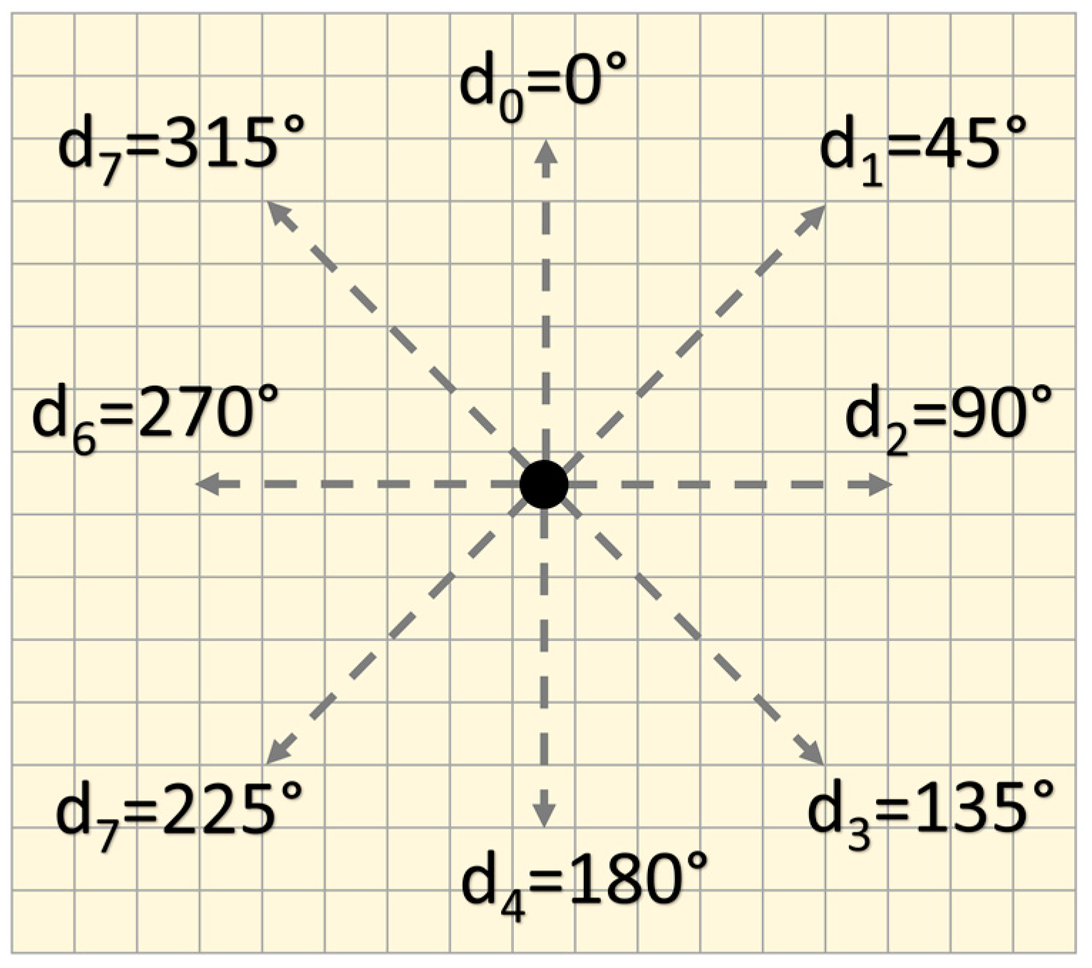
In order to capture bathymorphologic elements at the desired scales, the algorithm supports the definition of a search annulus contained between an internal radius () acting like a low-pass filter, and an external radius () that limits the extent of the spatial analysis. Although the node neighborhood may be potentially evaluated in any range of directions, exploratory tests have shown that limiting the analysis to eight directions () (the four cardinal directions and the four main inter-cardinal directions) provides a good working tradeoff between computation efficiency and stability of the retrieved information (Figure 1).
Adopting the described analytic schema, bathymorphons can only fall into a finite number of configurations based on the ternary nature of the LTP and the eight selected neighbor directions (Figure 2). Having three possible states for each of the eight directions, the number of possible LTP values is 6561 (). However, given the symmetry of many of these configurations, the actual number of unique bathymorphon classes, after having evaluated all the possible rotations and mirroring operations, is 498 [31]. Based on evidence from preliminary tests, some of these morphological seafloor types are very common, while others describe quite rare forms (an example of bathymorphon distribution is presented in Figure 3).
The evaluation on the assigned ternary level () per direction is based on the line-of-sight principle: two straight lines are passed connecting each DEM node to the “visible” highest and lowest node in each of the eight directions identified in Figure 1. The line-of-sight principle is implemented by using a user-defined parametric angular flatness threshold () and the difference between the zenith () and the nadir () angles (Figure 4) as defined in Equation (1):
Using and the described angular difference, each node is assigned to a bathymorphon class that expresses the degree of dominance or enclosure of a node location on an irregular surface (i.e., the openness) [30], at the user-identified scale (i.e., the search annulus). This line-of-sight approach has the advantage of reducing complications derived from having to manage the range of spatial scales that is often a limitation in approaches based on differential geometry.
As demonstrated in [31], the bathymorphons can be grouped into a relatively small (ten) number of landform classes that capture most the relevant morphologic relationships related to landform description. In our case we believe that the majority of the information can be captured by mapping the generated bathymorphons into six possible seafloor geoform classes, each representing a common bathymorphologic element, using the lookup table provided in Table 1. These six classes thus represent a simplification of the lookup table proposed in [31]. Pits and peaks present in [31] have been merged with valleys and ridges, respectively; and, the concave- and convex-slope cases describe in [34] redistributed among the slope, shoulder, and footslope classes provided in Table 1.
The lookup table step usually greatly reduces the complexity of the segmentation by at least one order of magnitude. The next step is the creation of area kernels, i.e., connected regions of common bathymorphon class. The area kernels are created by applying the connected components labeling algorithm (specifically, the Block Based with Decision Trees algorithm described in [36]) to the seafloor form-classified grid creating a bathy-morphometric map. This step of the algorithm scans the created map with bathymorphon classes, and groups its nodes into components based on node connectivity: all nodes in a connected component share same bathymorphon class and are connected with each other. Once all groups have been determined, each node is labeled according to the component it was assigned to.
The algorithm adopted for the definition of the area kernels can be summarized in the following four main steps applied to each node of the grid:
- Calculation of the ternary value based on neighborhood and search annulus.
- Reduction (by mirroring and rotating) of the ternary value to one of the 498 bathymorphon classes.
- Assignment of each bathymorphon to one of the six seafloor geoform classes through a user-modifiable lookup table (Table 1).
- Creation of the area kernels by clustering all the connected nodes within the same geoform class.
After preliminary tests, the described approach highlighted two possible distortions in the classification: nodes close to the edge of the surface, and in case of the selection of a large external radius for the search annulus. Two optional corrections have thus been identified and introduced: a “Node-on-the-Edge” correction that classifies only nodes that have a minimum number of valid ternary levels (default value adopted for this parameter is 6); and, an “extended-form” correction that stops, after a given distance, the effects of the angular flatness threshold on the resulting calculated elevation used to identify a “flat”.
2.2. Derivation of Seafloor Segments
In the second and final phase, the algorithm then evaluates each area kernel within the context of the backscatter mosaic much as an experienced analyst would use the backscatter to understand the context of given morphological regions. The region of each area kernel in the bathy-morphometric map is evaluated using only the co-located pixels in the acoustic backscatter mosaic. This evaluation is performed both in isolation (to assess the requirement subdividing into smaller area kernels), and by pairwise comparison to other area kernels of the same seafloor form type (to cluster area kernels with similar characteristics). Thus, the area kernels identified in the bathymetric realm are split or merged based on the intensity-level distribution of the pixels in the corresponding region in the mosaic. To maximize the robustness of this operation and avoid the introduction of biases, the acoustic backscatter mosaic has to be created using the best practices for radiometric and geometric corrections (e.g., the effect of local slope) and for normalization to minimize the angular dependency and possible artifacts in the collected reflectivity data [5,23].
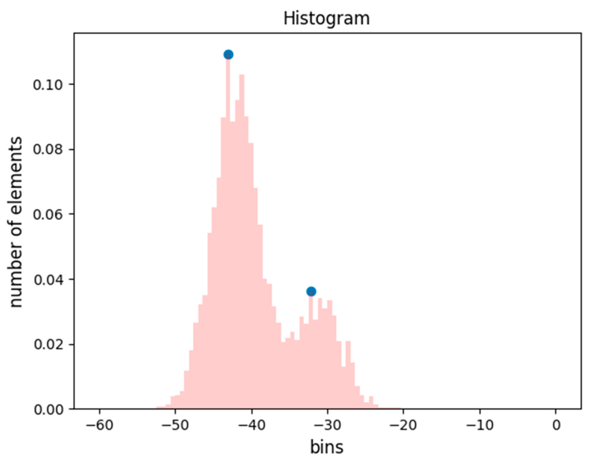
A normalized (45°), slope-corrected (by deriving the true incidence angle from DEM) intensity-level histogram for each individual area kernel is created and then analyzed to identify the possible presence of multiple modes (Figure 5). The process first identifies the index of the bin of the peak by taking the first order differences, then enhances the resolution of the peak detection by using Gaussian fitting, centroid computation [37,38]. The multi-modal detection is tailored by adopting two customizable parameters: is the amplitude threshold given as percentage of the total number of elements (that is, the peaks with amplitude lower than the given threshold are ignored) and represents the minimum distance between peaks. These parameters can be used to improve the algorithm robustness in case of the presence of small artifacts in the acoustic mosaic. The identification of more than one peak triggers the execution of a simple k-means algorithm [39], an unsupervised learning algorithm commonly used to solve the well-known clustering problem. This algorithm is used here to split the nodes belonging to a specific area kernel into a number of clusters defined by the identified peaks.
The evaluation in the pairwise comparison is performed through a simplified histogram comparison approach [40,41]. The percentage of intersection () between a pair of histograms is adopted as a criterion to evaluate whether the area kernel belonging to the same seafloor form type (e.g., a valley) has the same textural characteristics in the mosaic to be judged as representative of the same seafloor segment (Figure 6). The value used as the merging threshold varies based on the specific task that the algorithm is adopted for; however, initial tests have identified a validity range between 50% and 80%.
As a rule of thumb, backscatter data collected with modern multibeam echo sounders, typically produces a mosaic with resolution of 2–3 times the resolution of the corresponding bathymetric DEM. In order to apply the two described steps to area kernels with statistics that are stable, only area kernels of at least 10 nodes (corresponding at about 40 pixels on the mosaic) are evaluated. Area kernels smaller than this size are currently staged as unclassified.
3. Results
In order to test the described bathymetric and reflectivity-based estimation method for seafloor segmentation, we applied it to a well-studied bedform field in the mouth of the Piscataqua River, a well-mixed estuary between New Hampshire and Maine, USA. The area was selected because it has been the subject of numerous previous mapping efforts including studies of bedform migration [42], automated segmentation [10], and seafloor scattering models [43,44]. The study area is centered on a shallow, sandy sediment region, determined by multiple means (sonars, divers, and video observations) to be a rippled sand-wave field composed of largely medium to coarse sand and fine shell hash, surrounded by bedrock and gravelly channel sediments [10,42,44,45]. The bedform field is a persistent, elongated feature with its major axis oriented north-south along the main channel axis of the lowermost part of the Piscataqua River estuary [42].
The bathymetric DEM and the acoustic backscatter mosaic was constructed using data collected with a dual-head Kongsberg (Kongsberg, Norway) EM3002D multibeam echosounder (operating at 300-kHz central frequency and installed on the University of New Hampshire’s R/V Coastal Surveyor). Positioning and attitude data were collected from an Applanix (Richmond Hill, Ontario, Canada) POS/MV system with integrated real-time kinematic GPS. The bathymetric data were processed and gridded at a 0.5-m resolution using QPS Qimera (version 1.5.5) processing software (Quality Positioning Services BV, Zeist, The Netherland), while the backscatter mosaic was generated using Center for Coastal and Ocean Mapping (Durham, NH, USA)’s in-house research code [5,46] at 0.13-m resolution (Figure 7); backscatter is presented normalized to a 45 degree angle of incidence. Both products were created using a UTM 18N/WGS84 cartographic projection and stored in a portable ASCII grid format.
The BRESS algorithm is implemented mainly in C++11, with a graphical user interface created in Python. The implementation creates all the outputs (the final products and several optional intermediate layers) with the same shape and projection of the original bathymetric DEM. Although not required by the adopted set of input data, the code implementation is able to identify inputs with different projections and re-project the mosaic input to match the projection of the bathymetric input.
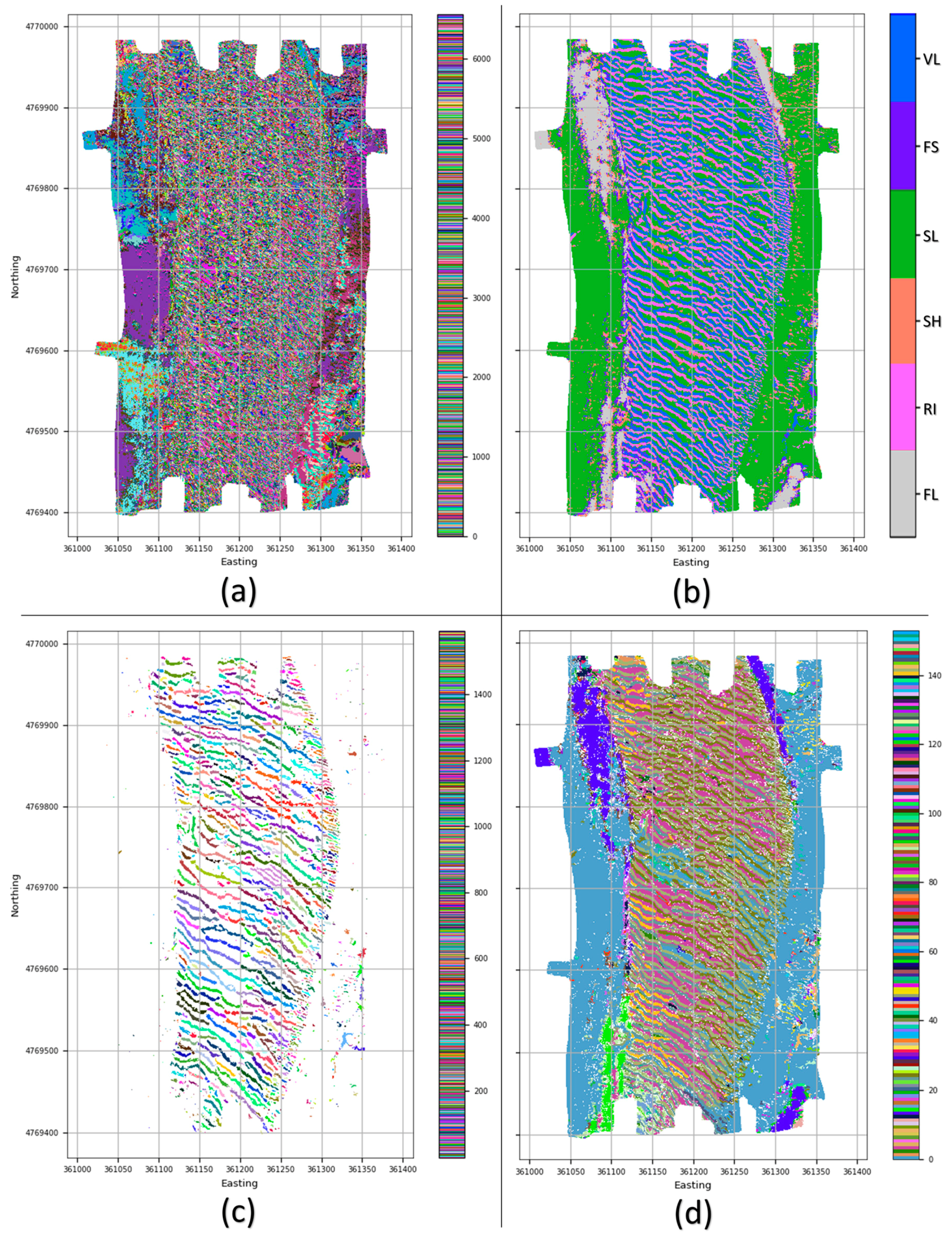
An example of the processing steps is shown in Figure 8. Figure 8a shows the initial LTP values calculated for each node in the DEM (with: , and ). Using this parameter set, the length scale of detectable features is between 1.5 and 5 m. Figure 8b shows the reduction of the original 6561 LPT values to the six seafloor geoform classes described in Table 1. All six of the geoform types are present in the dataset, and this representation shows a clear differentiation between the central rippled sand-wave field and the surrounding regions that matches nicely the manually-derived delineation of physiographic differences in the area [47,48]. For some applications, this simple segmentation based on bathymetry alone may be adequate. However, if an application requires information on sediment type (e.g., grain size), the bathymetrically-derived segmentation may not suffice. For instance, a flat seafloor that has various sediment types will likely end in a single seafloor geoform.
To bring in the context of the backscatter mosaic, the area kernels are then generated by clustering all the connected nodes within the same geoform class (valleys are shown in Figure 8c). Finally, each area kernel is analyzed in isolation to assess the need for sub-division into smaller area kernels (, ), and by pairwise comparison to other area kernels of the same seafloor form type () to generate the final segmentation in Figure 8d. The final segmentation provides the advantage of also capturing the effects of areas of different seafloor reflectivity (i.e., it shows whether the connected geoform segments (valleys in our example) are homogenous or segmented with respect to backscatter). By analyzing the different labels assigned within the same type of geoforms, it is now possible to identify detailed patterns of variability. By stopping the analysis at the area kernels in Figure 8b, the presence of these patterns would have been otherwise ignored.
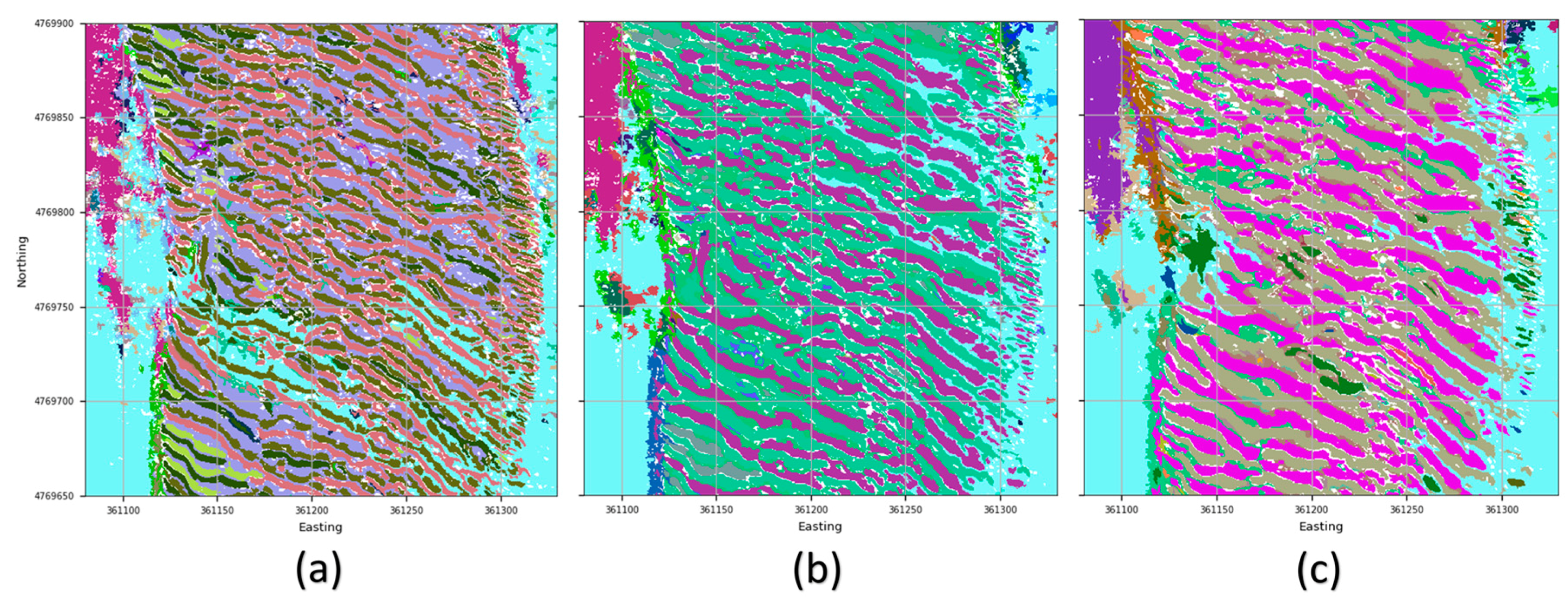
Figure 9 shows the impact of using different values for the search annulus for a portion of the study area presented in Figure 8. The portion area in Figure 9a presents a larger number of segments when compared to Figure 9b as the result of increasing the range of the search annulus (from , to , ), thus, by capturing only geoforms at a scale larger than 3 m. Although decreased, the effect of reduction in output complexity by increasing the search annulus is also present in Figure 9c. By changing the search parameters, the BRESS algorithm can be tuned for different usages and scenarios.
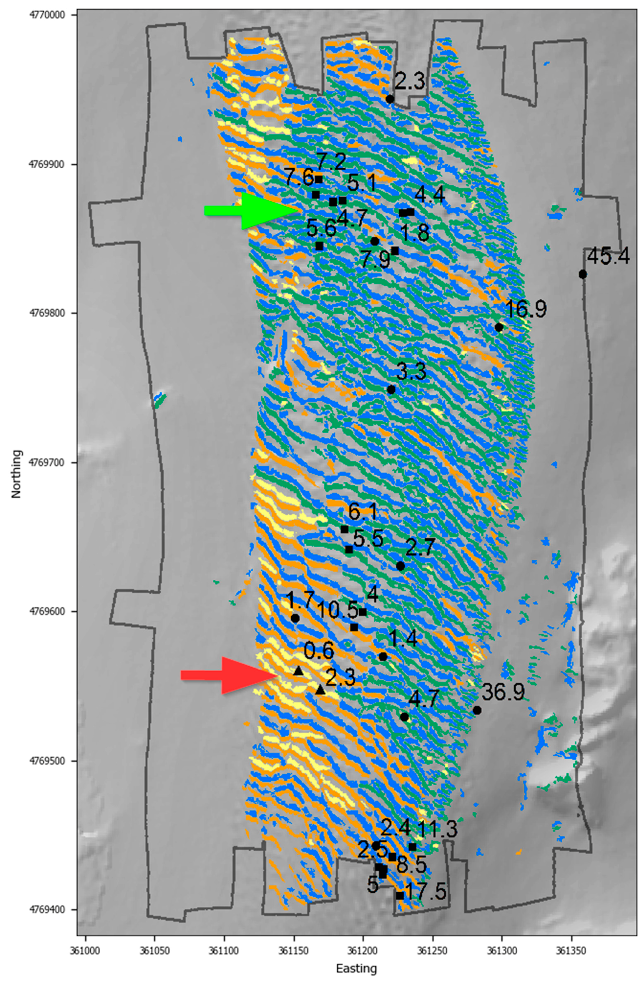
Finally, an exploratory evaluation of the advanced discrimination capabilities of the algorithm is presented in Figure 10. The region shown in Figure 10 is the rippled sand-wave field who’s central region is generally characterized as medium sand and that has been shown to be stable over the years [42,47]. Figure 10 shows just the “valley” and “ridge” bathymorphons in the area, in this case, the troughs and crests of the sand waves. The analysis of the backscatter of the valleys and the ridges shows that they vary in their reflectivity behavior in a spatially-consistent manner. For instance, the cluster of yellow (for valleys) and orange (for ridges) segments present in Figure 10 in the south-west region of the sand wave area (pointed by the red arrow) versus the cluster of blues (for valleys) and dark green (for ridges) segments in the central region (light green arrow). These clusters appear to correlate with the variations in the percentage of gravel and shells based on the limited ground-truth datasets available (Figure 10).
Although this correlation is promising, it is based on limited data collected for other purposes. With this new analysis, we can now (and will) test the discrimination capabilities of the algorithm by carefully designing a sampling plan to ground-truth the different segment types or test the fit-for-purpose for field-specific applications (e.g., the evaluation of seabed habitat maps presented in [49]). In fact, the collection of additional ground-truth values will provide means to evaluate the efficacy of the BRESS method in comparison with other available methods: for example, the Object Based Image Analysis applied to both MBES bathymetry and acoustic backscatter [19,20] or the combined use of the terrain attributes obtained with Benthic Terrain Modeler [14,50], and a parallel classification of the acoustic backscatter.
From a theoretical point of view, the BRESS method presents the key advantage of having both physically meaningful and statistically intuitive (intermediate and final) steps. In other words, the processing steps can be translated into relatively simple questions (e.g., what geoform class does this DEM node belong to? Which range of scales is the target of the analysis? By looking at the reflectivity content, is a specific pair of area kernels similar?). This intuitiveness should facilitate its adoption and proper use, while other existing methods often require quite abstract evaluations (e.g., the tuning of “magic numbers” used as parameters) or deep statistical insights on the study area. The amount of local, specific knowledge often required by methods like [19] and [50] makes them difficult to be ported, with a consistent success classification rate, to different study areas. The evaluation of the BRESS method in comparison with those methods should also consider such factors.
4. Conclusions
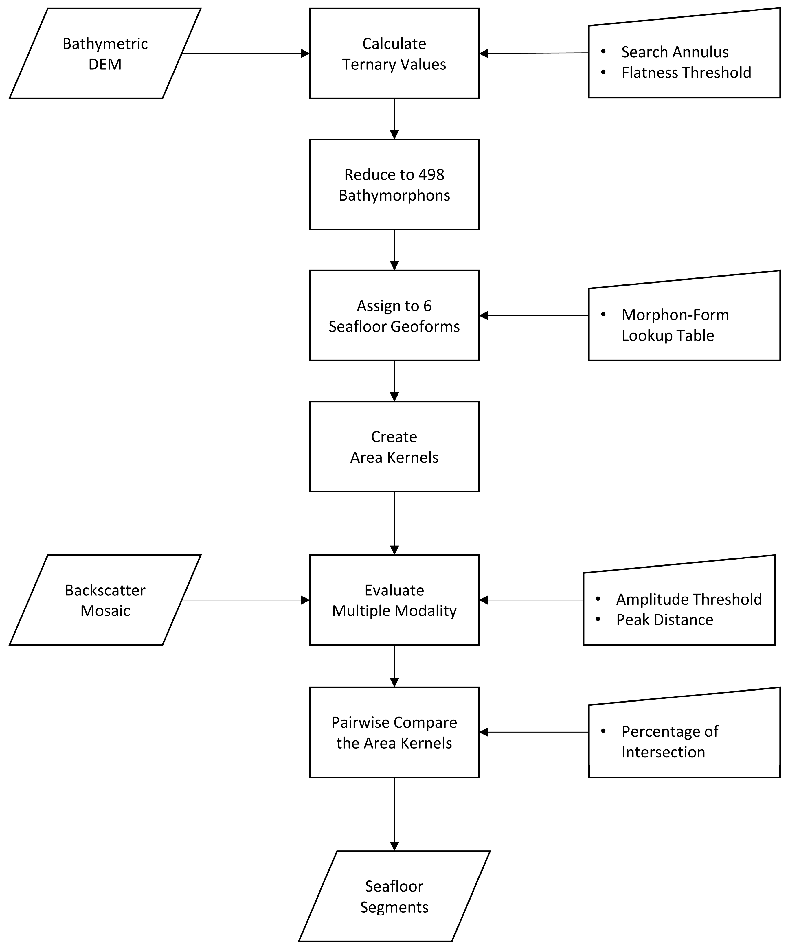
BRESS offers a novel approach for the quantitative analysis of ocean mapping data. The incentive for developing this method was a desire to create an automated, scale-independent, robust and computationally efficient technique to segment the seafloor for a range of research applications. The method differs from standard approaches that tend to use either bathymetry or backscatter data independently in that it attempts to emulate the approach of a skilled analyst by using the full context of both the bathymetry and the backscatter (Figure 11 summarizes the algorithm workflow).
From a bathymetric perspective, the adoption of the concept of grid openness (using thresholds of flatness) makes the algorithm self-adaptive within the identified search annulus, with a clear gain in computational efficiency [31]. On the acoustic reflectivity side, the derivation of the seafloor segments based on local normalized histograms makes the method robust in the presence of the many possible artifacts that could be present in an acoustic backscatter mosaic [46,51]. The optional corrections, “Node-on-the-Edge” and “Extended-Form”, improve the overall algorithm robustness for cases in which the general approach was shown to have possible weaknesses.
The output of BRESS is a collection of homogeneous, non-overlapping seafloor segments. Each labeled segment is enriched by a list of derived, physically-meaningful attributes that can be used for subsequent task-specific analysis. The ability to natively perform a multi-scale analysis through a prescribed search annulus mitigates the risk of mismatch of spatial scales between measurements and their interpretation. Although the method cannot overcome the limitations that result from the inherent resolution of the system used for data collection [52], recent developments in acoustic mapping systems are currently achieving an unprecedented high-resolution view of the seafloor at a broad range of spatial scales. In particular, modern multibeam echosounders may produce continuous coverage depth measurements and co-located, high-quality reflectivity measurements that reveal well-defined texture patterns.
The described method is able to identify patterns of seafloor topography representing areas of homogenous geomorphological feature types and seafloor textures remotely sensed by acoustic devices. Given the relevance of this information to the spatial distributions of habitats, we believe that the method has a potential application for habitat mapping. Although habitat delineations can be done manually, robust automated procedures, like the BRESS method, offer increased speed, efficiency, more objectivity, and reproducible map products. Another possible application is to improve the understanding of seafloor stability, particularly important in the coastal environment [53]. In fact, the quality of the identification of valleys and ridges within a defined range of scales makes BRESS outputs a good candidate for use in the calculation of bedform migration rates. Finally, another potential application is its adoption as a source of acoustic themes for seafloor characterization by backscatter model inversion [54].
Acknowledgments
This work was supported by the NOAA grant NA15NOS4000200.
Author Contributions
Giuseppe Masetti and Larry Alan Mayer conceived and designed the algorithm; and Larry Guy Ward contributed to its improvement and to the analysis of the results.
Conflicts of Interest
The authors declare no conflict of interest. The founding sponsors had no role in the design of the study; in the collection, analyses, or interpretation of data; in the writing of the manuscript; or in the decision to publish the results.
References
- De Moustier, C.; Alexandrou, D. Angular dependence of 12-khz seafloor acoustic backscatter. J. Acoust. Soc. Am. 1991, 90, 522–531. [Google Scholar] [CrossRef]
- Hughes Clarke, J.E.; Mayer, L.A.; Wells, D.E. Shallow-water imaging multibeam sonars: A new tool for investigating seafloor processes in the coastal zone and on the continental shelf. Mar. Geophys. Res. 1996, 18, 607–629. [Google Scholar] [CrossRef]
- Augustin, J.; Dugelay, S.; Lurton, X.; Voisset, M. Applications of an image segmentation technique to multibeam echo-sounder data. In Proceedings of the OCEANS’97, MTS/IEEE Conference Proceedings, Halifax, NS, Canada, 6–9 October 1997; pp. 1365–1369. [Google Scholar]
- Rzhanov, Y.; Fonseca, L.; Mayer, L. Construction of seafloor thematic maps from multibeam acoustic backscatter angular response data. Comput. Geosci. 2012, 41, 181–187. [Google Scholar] [CrossRef]
- Fonseca, L.; Mayer, L. Remote estimation of surficial seafloor properties through the application angular range analysis to multibeam sonar data. Mar. Geophys. Res. 2007, 28, 119–126. [Google Scholar] [CrossRef]
- Lamarche, G.; Lurton, X.; Verdier, A.L.; Augustin, J.M. Quantitative characterisation of seafloor substrate and bedforms using advanced processing of multibeam backscatter—Application to cook strait, New Zealand. Cont. Shelf Res. 2011, 31, S93–S109. [Google Scholar] [CrossRef]
- De, C.; Chakraborty, B. Model-based acoustic remote sensing of seafloor characteristics. IEEE Trans. Geosci. Remote Sens. 2011, 49, 3868–3877. [Google Scholar] [CrossRef]
- Kloser, R.J.; Penrose, J.D.; Butler, A.J. Multi-beam backscatter measurements used to infer seabed habitats. Cont. Shelf Res. 2010, 30, 1772–1782. [Google Scholar] [CrossRef]
- Masetti, G.; Calder, B. Remote identification of a shipwreck site from mbes backscatter. J. Environ. Manag. 2012, 111, 44–52. [Google Scholar] [CrossRef] [PubMed]
- Cutter, G.R.; Rzhanov, Y.; Mayer, L.A. Automated segmentation of seafloor bathymetry from multibeam echosounder data using local fourier histogram texture features. J. Exp. Mar. Biol. Ecol. 2003, 285, 355–370. [Google Scholar] [CrossRef]
- Malinverno, A. Segmentation of topographic profiles of the seafloor based on a self-affine model. IEEE J. Ocean. Eng. 1989, 14, 348–359. [Google Scholar] [CrossRef]
- Wilson, M.F.J.; O’Connell, B.; Brown, C.; Guinan, J.C.; Grehan, A.J. Multiscale terrain analysis of multibeam bathymetry data for habitat mapping on the continental slope. Mar. Geod. 2007, 30, 3–35. [Google Scholar] [CrossRef]
- Dolan, M.; Thorsnes, T.; Leth, J.; Al-Hamdani, Z.; Guinan, J.; Van Lancker, V. Terrain Characterization from Bathymetry Data at Various Resolutions in European Waters—Experiences and Recommendations. Available online: https://www.ngu.no/en/publikasjon/terrain-characterization-bathymetry-data-various-resolutions-european-waters-experiences (accessed on 4 January 2018).
- Lundblad, E.R.; Wright, D.J.; Miller, J.; Larkin, E.M.; Rinehart, R.; Naar, D.F.; Donahue, B.T.; Anderson, S.M.; Battista, T. A benthic terrain classification scheme for american samoa. Mar. Geod. 2006, 29, 89–111. [Google Scholar] [CrossRef]
- Zarai, M.; Boudraa, A.O.; Garlan, T.; Thibaud, R.; Ray, C. Seafloor characterization by bathymetric image segmentation. In Proceedings of the OCEANS, Shanghai, China, 10–13 April 2016; pp. 1–4. [Google Scholar]
- Pirtle, J.L.; Weber, T.C.; Wilson, C.D.; Rooper, C.N. Assessment of trawlable and untrawlable seafloor using multibeam-derived metrics. Methods Oceanogr. 2015, 12, 18–35. [Google Scholar] [CrossRef]
- Lawrence, E.; Hayes, K.R.; Lucieer, V.L.; Nichol, S.L.; Dambacher, J.M.; Hill, N.A.; Barrett, N.; Kool, J.; Siwabessy, J. Mapping habitats and developing baselines in offshore marine reserves with little prior knowledge: A critical evaluation of a new approach. PLoS ONE 2015, 10, e0141051. [Google Scholar] [CrossRef] [PubMed]
- Chakraborty, B.; Menezes, A.; Dandapath, S.; Fernandes, W.A.; Karisiddaiah, S.; Haris, K.; Gokul, G. Application of hybrid techniques (self-organizing map and fuzzy algorithm) using backscatter data for segmentation and fine-scale roughness characterization of seepage-related seafloor along the western continental margin of india. IEEE J. Ocean. Eng. 2015, 40, 3–14. [Google Scholar] [CrossRef]
- Lucieer, V.; Lamarche, G. Unsupervised fuzzy classification and object-based image analysis of multibeam data to map deep water substrates, cook strait, new zealand. Cont. Shelf Res. 2011, 31, 1236–1247. [Google Scholar] [CrossRef]
- Lacharité, M.; Brown, C.J.; Gazzola, V. Multisource multibeam backscatter data: Developing a strategy for the production of benthic habitat maps using semi-automated seafloor classification methods. Mar. Geophys. Res. 2017, 1–16. [Google Scholar] [CrossRef]
- Brown, C.J.; Blondel, P. Developments in the application of multibeam sonar backscatter for seafloor habitat mapping. Appl. Acoust. 2009, 70, 1242–1247. [Google Scholar] [CrossRef]
- Tang, Q.H.; Zhou, X.H.; Liu, Z.C.; Du, D.-W. Processing multibeam backscatter data. Mar. Geod. 2005, 28, 251–258. [Google Scholar] [CrossRef]
- Lurton, X.; Lamarche, G.; Brown, C.; Lucieer, V.; Rice, G.; Schimel, A.; Weber, T. Backscatter Measurements by Seafloor-Mapping Sonars: Guidelines and Recommendations; A collective report by members of the GeoHab Backscatter Working Group; GeoHab Backscatter Working Group: Salvador da Bahia, Brazil, May 2015. [Google Scholar]
- Lecours, V.; Dolan, M.F.; Micallef, A.; Lucieer, V.L. A review of marine geomorphometry, the quantitative study of the seafloor. Hydrol. Earth Syst. Sci 2016, 20, 3207–3244. [Google Scholar] [CrossRef]
- Saadat, H.; Bonnell, R.; Sharifi, F.; Mehuys, G.; Namdar, M.; Ale-Ebrahim, S. Landform classification from a digital elevation model and satellite imagery. Geomorphology 2008, 100, 453–464. [Google Scholar] [CrossRef]
- Bishop, M.P.; James, L.A.; Shroder, J.F.; Walsh, S.J. Geospatial technologies and digital geomorphological mapping: Concepts, issues and research. Geomorphology 2012, 137, 5–26. [Google Scholar] [CrossRef]
- Lecours, V.; Devillers, R.; Schneider, D.C.; Lucieer, V.L.; Brown, C.J.; Edinger, E.N. Spatial scale and geographic context in benthic habitat mapping: Review and future directions. Mar. Ecol. Prog. Ser. 2015, 535, 259–284. [Google Scholar] [CrossRef]
- Grohmann, C.H.; Smith, M.J.; Riccomini, C. Multiscale analysis of topographic surface roughness in the midland valley, Scotland. IEEE Trans. Geosci. Remote Sens. 2011, 49, 1200–1213. [Google Scholar] [CrossRef]
- Wu, J. Effects of changing scale on landscape pattern analysis: Scaling relations. Landsc. Ecol. 2004, 19, 125–138. [Google Scholar] [CrossRef]
- Yokoyama, R.; Shirasawa, M.; Pike, R.J. Visualizing topography by openness: A new application of image processing to digital elevation models. Photogramm. Eng. Remote Sens. 2002, 68, 257–266. [Google Scholar]
- Jasiewicz, J.; Stepinski, T.F. Geomorphons—a pattern recognition approach to classification and mapping of landforms. Geomorphology 2013, 182, 147–156. [Google Scholar] [CrossRef]
- Liao, W.H. Region description using extended local ternary patterns. In Proceedings of the 2010 20th International Conference on Pattern Recognition (ICPR), Istanbul, Turkey, 23–26 August 2010; pp. 1003–1006. [Google Scholar]
- Julesz, B. A brief outline of the texton theory of human-vision. Trends Neurosci. 1984, 7, 41–45. [Google Scholar] [CrossRef]
- Ojala, T.; Pietikäinen, M.; Mäenpää, T. Gray scale and rotation invariant texture classification with local binary patterns. In Proceedings of the 6th European Conference on Computer Vision Dublin, Dublin, Ireland, 26 June–1 July 2000; pp. 404–420. [Google Scholar]
- Alvarez, S.; Vanrell, M. Texton theory revisited: A bag-of-words approach to combine textons. Pattern Recognit. 2012, 45, 4312–4325. [Google Scholar] [CrossRef]
- Grana, C.; Borghesani, D.; Cucchiara, R. Optimized block-based connected components labeling with decision trees. IEEE Trans. Image Process. 2010, 19, 1596–1609. [Google Scholar] [CrossRef] [PubMed]
- Sezan, M.I. A peak detection algorithm and its application to histogram-based image data reduction. Comput. Vis. Graph. Image Process. 1990, 49, 36–51. [Google Scholar] [CrossRef]
- Abdel-Aal, R.E. Comparison of algorithmic and machine learning approaches for the automatic fitting of gaussian peaks. Neural Comput. Appl. 2002, 11, 17–29. [Google Scholar] [CrossRef]
- MacQueen, J. Some methods for classification and analysis of multivariate observations. In Proceedings of the fifth Berkeley Symposium on Mathematical Statistics and Probability, Oakland, CA, USA, 21 June–18 July 1965; pp. 281–297. [Google Scholar]
- Barla, A.; Odone, F.; Verri, A. Histogram intersection kernel for image classification. In Proceedings of the 2003 International Conference on Image Processing—ICIP 2003, Barcelona, Spain, 14–17 September 2003; p. III-513. [Google Scholar]
- Boughorbel, S.; Tarel, J.-P.; Boujemaa, N. Generalized histogram intersection kernel for image recognition. Proceeding of the 2005 12th IEEE International Conference on Image Processing (ICIP 2005), Genova, Italy, 11–14 September 2005; p. III-161. [Google Scholar]
- Felzenberg, J.A. Detecting Bedform Migration from Gigh-Resolution Multibeam Bathymetry in Portsmouth Harbor, New Hampshire, USA. Master’s Thesis, University of New Hampshire, Durham, NH, USA, September 2009. [Google Scholar]
- Weber, T.C.; Ward, L.G. Observations of backscatter from sand and gravel seafloors between 170 and 250 khz. J. Acoust. Soc. Am. 2015, 138, 2169–2180. [Google Scholar] [CrossRef] [PubMed]
- Weber, T.C.; Ward, L. High-frequency seafloor scattering in a dynamic harbor environment: Observations of change over time scales of seconds to seasons. J. Acoust. Soc. Am. 2016, 140, 3348–3349. [Google Scholar] [CrossRef]
- Nifong, K.L. Sedimentary Environments and Depositional History of a Paraglacial, Estuarine Embayment and Adjacent Inner Continental Shelf: Portshmouth Harbor, New Hampshire, USA. Master’s Thesis, University of New Hampshire, Durham, NH, USA, December 2016. [Google Scholar]
- Masetti, G.; Calder, B.R.; Hughes Clarke, J.E. Methods for artifact identification and reduction in acoustic backscatter mosaicking. In Proceedings of the U.S. Hydro 2017 Conference, Galveston, TX, USA, 20–23 March 2017. [Google Scholar]
- Ward, L.G. Sedimentology of the Lower Great Bay/Piscataqua River Estuary; Final Report, Revision 1; Jackson Estuarine Laboratory, University of New Hampshire: Durham, NH, USA, 1995. [Google Scholar]
- Ward, L.G.; Zaprowski, B.J.; Trainer, K.D.; Davis, P.T. Stratigraphy, pollen history and geochronology of tidal marshes in a gulf of maine estuarine system: Climatic and relative sea level impacts. Mar. Geol. 2008, 256, 1–17. [Google Scholar] [CrossRef]
- Diesing, M.; Green, S.L.; Stephens, D.; Lark, R.M.; Stewart, H.A.; Dove, D. Mapping seabed sediments: Comparison of manual, geostatistical, object-based image analysis and machine learning approaches. Cont. Shelf Res. 2014, 84, 107–119. [Google Scholar] [CrossRef] [Green Version]
- Arcgis Benthic Terrain Modeler (BTM); version 5.1; NOAA Office for Coastal Management: Charleston, SC, USA, 2012.
- Hughes Clarke, J.E.; Li, M.Z.; Sherwood, C.R.; Hill, P.R. Optimal use of multibeam technology in the study of shelf morphodynamics. In Sediments, Morphology and Sedimentary Processes on Continental Shelves: Advances in Technologies, Research and Applications, 1st ed.; International Association of Sedimentologists: Gent, Belgium, 2013; pp. 3–28. [Google Scholar]
- Lurton, X.; Eleftherakis, D.; Augustin, J.M. Analysis of seafloor backscatter strength dependence on the survey azimuth using multibeam echosounder data. Mar. Geophys. Res. 2017. [Google Scholar] [CrossRef]
- Nittrouer, J.A.; Allison, M.A.; Campanella, R. Bedform transport rates for the lowermost Mississippi River. J. Geophys. Res. Earth Surf. 2008, 113, 1–16. [Google Scholar] [CrossRef]
- Fonseca, L.; Brown, C.; Calder, B.; Mayer, L.; Rzhanov, Y. Angular range analysis of acoustic themes from stanton banks ireland: A link between visual interpretation and multibeam echosounder angular signatures. Appl. Acoust. 2009, 70, 1298–1304. [Google Scholar] [CrossRef]
Figure 1.
Selected eight directions () surrounding a DEM node in solid black. Each direction is evaluated independently by only taking into account the neighborhood nodes between the search annulus identified by the internal () and external radii ().
Figure 1.
Selected eight directions () surrounding a DEM node in solid black. Each direction is evaluated independently by only taking into account the neighborhood nodes between the search annulus identified by the internal () and external radii ().

Figure 2.
Example of LTP evaluation surrounding a DEM node whereas a “+” is used to identify a “shoal”, a “0” for “flat”, and a “-“ for “deep” configurations, respectively. Following the convention described in the text, those levels are translated in a ternary value: a ternary digit (“-” = 0, “0” = 1, “+” = 2) for each of the eight directions (the “22210011” code in the example provided). The ternary value will then be reduced to one of the possible 498 bathymorphon classes.
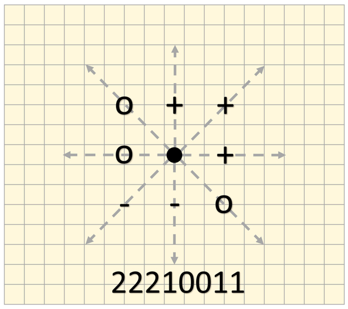
Figure 3.
Histogram providing the distribution of the bathymorphon classes for the testing dataset described in the Results section.
Figure 3.
Histogram providing the distribution of the bathymorphon classes for the testing dataset described in the Results section.
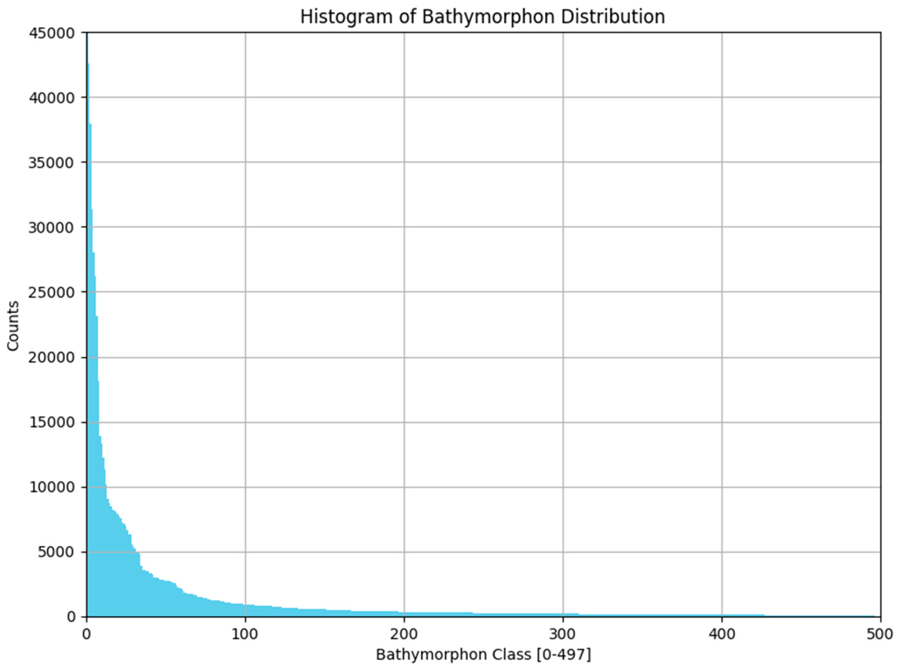
Figure 4.
A simplified, two-dimensional representation of DEM nodes (represented by black dots) and the underline the real surface (blue line). In particular, the large black dot represents the currently evaluated node, while the smaller dots are nodes in its surrounding, along the same direction. The line-of-sight principle is adopted to define the node openness in terms of zenith () and nadir () angles. Both angles are defined to be always positive, within a range from 0° to 180°. The difference among the two angles is used to define the ternary level in each node direction.

Figure 5.
Each individual area kernel is analyzed to detect the presence of multi-modal distribution. The figure shows an example with a bi-modal distribution (the two peaks are represented as blue dots). The bin values represent decibel values, but the same approach can be adopted by adapting the bins to dimensionless digital numbers. The number of elements is normalized.

Figure 6.
The histogram intersection is used as a criterion to compare pair of area kernels. The figure shows an example whereas the two normalized histograms overlap for more than 71% and are, thus, considered to come from seafloor with similar acoustic response.
Figure 6.
The histogram intersection is used as a criterion to compare pair of area kernels. The figure shows an example whereas the two normalized histograms overlap for more than 71% and are, thus, considered to come from seafloor with similar acoustic response.
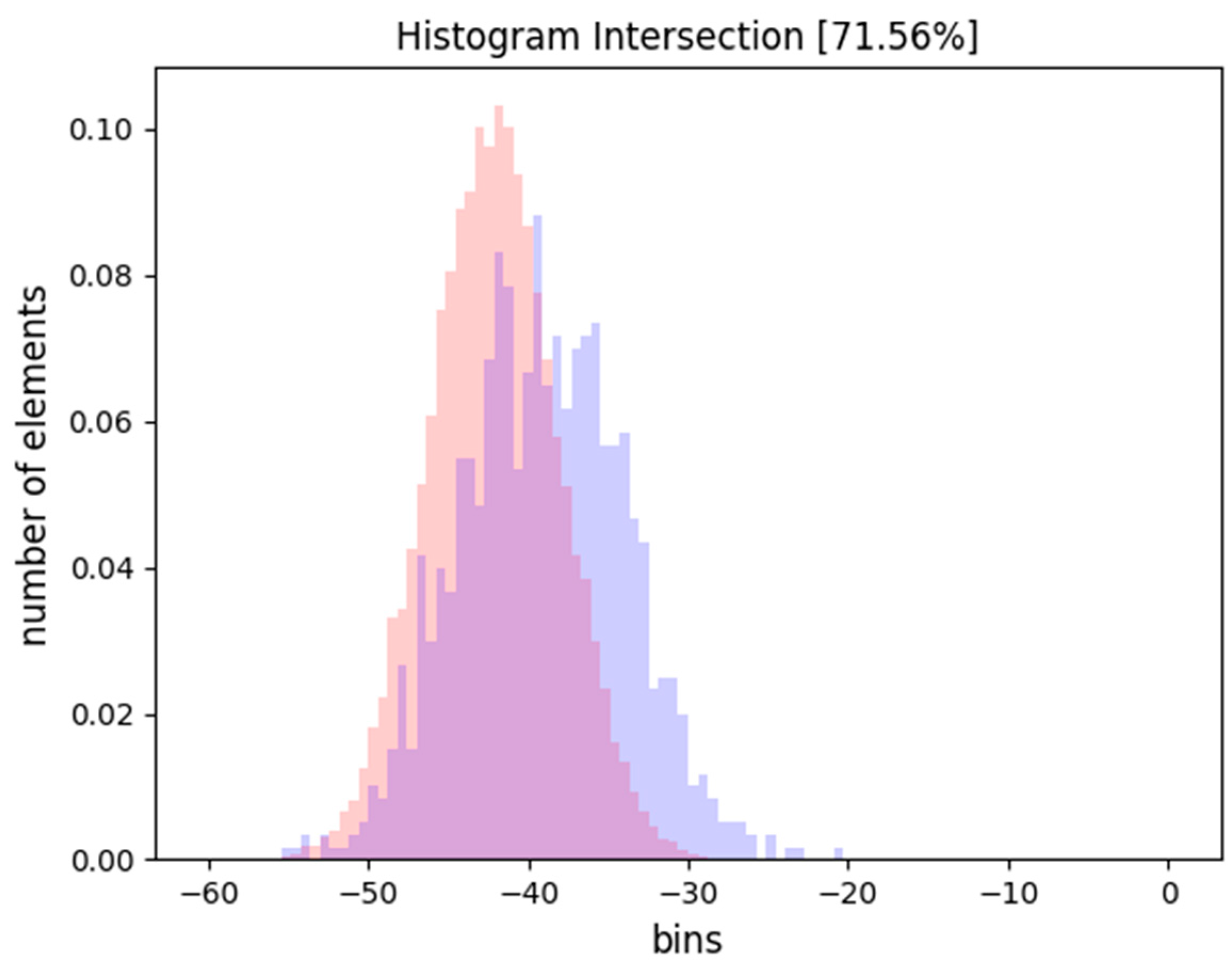
Figure 7.
Test data inputs collected over a bedform field located in the mouth of the Piscataqua River, USA. (a) Bathymetric DEM with a 50-cm resolution. (b) Acoustic backscatter mosaic assembled at 13-cm resolution.
Figure 7.
Test data inputs collected over a bedform field located in the mouth of the Piscataqua River, USA. (a) Bathymetric DEM with a 50-cm resolution. (b) Acoustic backscatter mosaic assembled at 13-cm resolution.
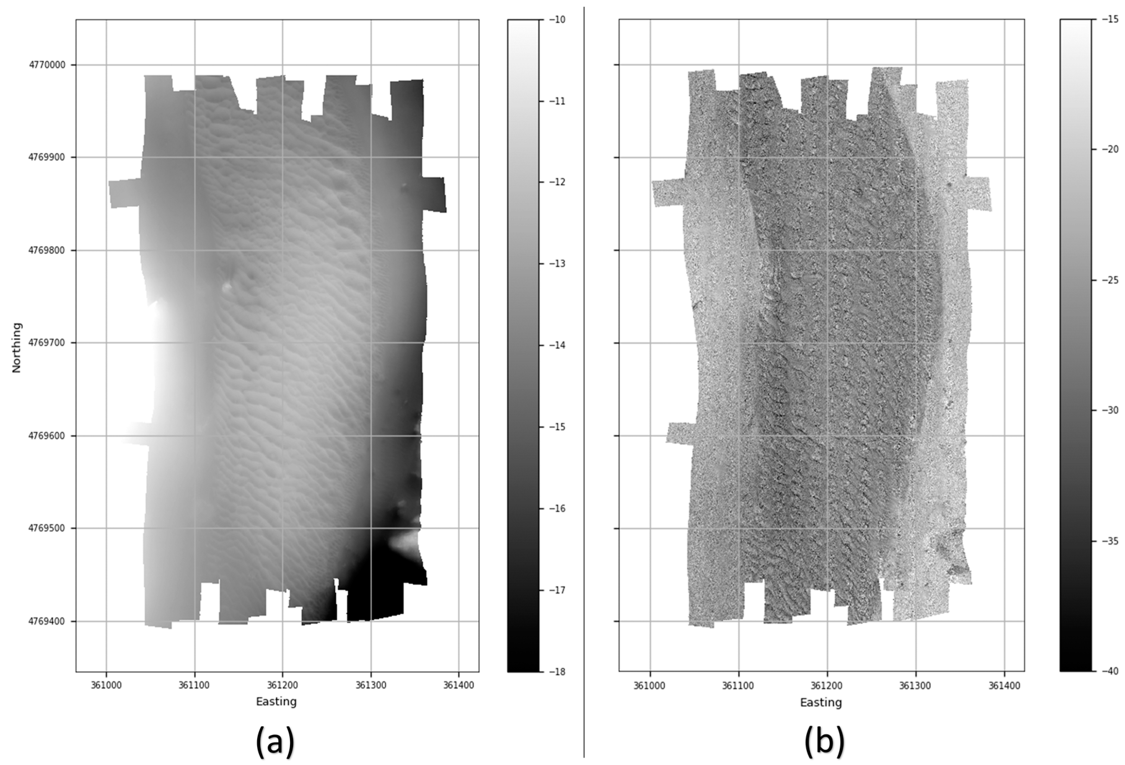
Figure 8.
The four major steps of the BRESS algorithm. (a) A ternary value is associated to each node of the DEM. (b) The 6561 (38) possible ternary values are first reduced to the 498 bathymorphons, then mapped to six geoform classes of interest (abbreviations defined in Table 1). (c) The area kernels are created by clustering all the connected nodes within the same geoform class (valley in the shown examples). Each area kernel has assigned a random color. (d) The output seafloor segments are generated by analyzing each area kernel in isolation, to assess the requirement of its sub-division in smaller area kernels, and by pairwise comparison to other area kernels of the same geoform type.

Figure 9.
The three insets show, on a central portion of the study area, the effects of adopting search annuli of increasing size: (a) , ; (b) , ; and (c) , . A direct effect of such variation is a reduction on the number of output segments for the whole study area: (a) 154, (b) 118, and (c) 96.
Figure 9.
The three insets show, on a central portion of the study area, the effects of adopting search annuli of increasing size: (a) , ; (b) , ; and (c) , . A direct effect of such variation is a reduction on the number of output segments for the whole study area: (a) 154, (b) 118, and (c) 96.

Figure 10.
Algorithm segmentation output for valley (in yellow and blue) and ridge (in orange and green) geoforms compared with collected samples. The numerical values shown represent the percentage of gravel in the retrieved sediments. The samples were collected by three different studies that are represented using different symbol shapes: the circles for [42]; the squares for [44]; and the triangles for [45]. Shaded bathymetric relief is shown as the background and the survey polygon of the whole test area is represented with a gray line. The light green arrow and the red arrow point to areas with relatively high and low percentages of gravel and shells, respectively.

Figure 11.
Flowchart identifying the main inputs, outputs, and processing steps of the BRESS algorithm.
Figure 11.
Flowchart identifying the main inputs, outputs, and processing steps of the BRESS algorithm.


Table 1.
Lookup table adopted to map the bathymorphons (listed on the left inset together with their abbreviations) to the six seafloor form classes of interest for this step of the segmentation. Given the possibility of having a neutral level (a “flat”), the number of “shoals” and “deeps” surrounding the node point may vary between zero and eight. The header row and column provide the total number of positive and negative levels (respectively) for the eight directions surrounding each node. FL = Flat, RI = Ridge, SH = Shoulder, SL = Slope, FS = Footslope, VL = Valley.
| + | 0 | 1 | 2 | 3 | 4 | 5 | 6 | 7 | 8 | |
|---|---|---|---|---|---|---|---|---|---|---|
| − | ||||||||||
| 0 | FL | FL | FL | FS | FS | VL | VL | VL | VL | |
| 1 | FL | FL | FS | FS | FS | VL | VL | VL | - | |
| 2 | FL | SH | SL | SL | SL | VL | VL | - | - | |
| 3 | SH | SH | SL | SL | SL | SL | - | - | - | |
| 4 | SH | SH | SH | SL | SL | - | - | - | - | |
| 5 | RI | RI | RI | SL | - | - | - | - | - | |
| 6 | RI | RI | RI | - | - | - | - | - | - | |
| 7 | RI | RI | - | - | - | - | - | - | - | |
| 8 | RI | - | - | - | - | - | - | - | - | |
© 2018 by the authors. Licensee MDPI, Basel, Switzerland. This article is an open access article distributed under the terms and conditions of the Creative Commons Attribution (CC BY) license (http://creativecommons.org/licenses/by/4.0/).
Share and Cite
MDPI and ACS Style
Masetti, G.; Mayer, L.A.; Ward, L.G. A Bathymetry- and Reflectivity-Based Approach for Seafloor Segmentation. Geosciences 2018, 8, 14. https://doi.org/10.3390/geosciences8010014
AMA Style
Masetti G, Mayer LA, Ward LG. A Bathymetry- and Reflectivity-Based Approach for Seafloor Segmentation. Geosciences. 2018; 8(1):14. https://doi.org/10.3390/geosciences8010014
Chicago/Turabian StyleMasetti, Giuseppe, Larry Alan Mayer, and Larry Guy Ward. 2018. "A Bathymetry- and Reflectivity-Based Approach for Seafloor Segmentation" Geosciences 8, no. 1: 14. https://doi.org/10.3390/geosciences8010014
Note that from the first issue of 2016, this journal uses article numbers instead of page numbers. See further details here.