Article

Automated Webcam Monitoring of Fractional Snow Cover in Northern Boreal Conditions

1
Finnish Meteorological Institute (FMI), Erik Palménin aukio 1, FI-00560 Helsinki, Finland
2
Finnish Environment Institute Finland (SYKE), Mechelininkatu 34a, FI-00251 Helsinki, Finland
3
Natural Resources Institute Finland (LUKE), Viikinkaari 4, FI-00790 Helsinki, Finland
*
Authors to whom correspondence should be addressed.
Geosciences 2017, 7(3), 55; https://doi.org/10.3390/geosciences7030055
Submission received: 31 May 2017 / Revised: 28 June 2017 / Accepted: 4 July 2017 / Published: 9 July 2017
(This article belongs to the Special Issue Cryosphere)

Abstract

:
Fractional snow cover (FSC) is an important parameter to estimate snow water equivalent (SWE) and surface albedo important to climatic and hydrological applications. The presence of forest creates challenges to retrieve FSC accurately from satellite data, as forest canopy can block the sensor’s view of snow cover. In addition to the challenge related to presence of forest, in situ data of FSC—necessary for algorithm development and validation—are very limited. This paper investigates the estimation of FSC using digital imagery to overcome the obstacle caused by forest canopy, and the possibility to use this imagery in the validation of FSC derived from satellite data. FSC is calculated here using an algorithm based on defining a threshold value according to the histogram of an image, to classify a pixel as snow-covered or snow-free. Images from the MONIMET camera network, producing a continuous image series in Finland, are used in the analysis of FSC. The results obtained from automated image analysis of snow cover are compared with reference data estimated by visual inspection of same images. The results show the applicability and usefulness of digital imagery in the estimation of fractional snow cover in forested areas, with a Root Mean Squared Error (RMSE) in the range of 0.1–0.3 (with the full range of 0–1).

1. Introduction

Snow cover is an essential climate variable directly affecting the Earth’s energy balance, due to its high albedo. Snow cover has a number of important physical properties that exert an influence on global and regional energy, water supply, and carbon cycles. Its quantification in a changing climate is thus important for various environmental and economic impact assessments. Proper description and assimilation of snow cover information into hydrological, land surface, meteorological, and climate models, are critical to address the impact of snow on various phenomena, to predict local snow water resources, and to warn about snow-related natural hazards.
Several methods for retrieving fractional snow cover (FSC) from remote sensing data have been developed [1,2,3,4,5,6,7]. Boreal forest occupies about 17 percent of the Earth’s land surface area in a circumpolar belt in the far northern hemisphere. The presence of forest in seasonally snow-covered regions, especially in the northern hemisphere, creates great challenges for the accurate FSC retrieval from satellites, as forest canopy can block sensor’s view of snow cover, either almost totally, or at least partially. Many studies have been conducted to overcome the presence of forest [8,9,10,11,12,13].
In addition to the challenges of retrieval methodologies of remote sensing over forested areas, in situ data of FSC is rarely available, or at least temporally very limited. Ground reference data feasible for evaluation of FSC retrievals is often relatively difficult to obtain. This is because FSC is typically registered by human observers. Also, the use of very high resolution satellite images is complicated, as there are no feasible algorithms available to create a reliable and accurate FSC map for forested areas [14]. Moreover, fractional snow cover typically varies rather widely in space and time, and therefore single point observations are not necessarily representative of the local spatial variation. This representation also depends on the landscape characteristics and other prevailing conditions. The observations should be conducted over an area corresponding to the pixel size of the applied satellite sensor, and the timing should match the satellite overpass, at least so that no major changes in snow cover occur.
Several webcam networks intended for scientific monitoring of ecosystems have been established lately. The European Phenology Camera Network (EUROPhen) is a collection of cameras used for phenology across Europe [15]. In a similar way, the PhenoCam Network has more than 80 cameras across the US [16]. Time-lapse digital camera images of Australian biomes for different locations are archived and distributed by the Australian Phenocam Network [17]. The Phenological Eyes Network (PEN) is another phenological camera network in Asia [18]. The MONIMET camera network is established to provide time series of field observations, and consists of 27 cameras over Finland, presently distributed at 14 sites [19]. Digital images and other phenological data from such camera networks are used in various studies [15,16,18,20,21,22]. The use of digital repeat photography at a daily resolution can aid the automatic identification of interannual variations in vegetation status, and capture of agricultural practices [15]. Digital photos can be used for detecting phenological patterns quantitatively in various types of vegetation over a longer period [20]. Digital repeat photography can be used to assess the link between vegetation phenology and CO2 exchange for two high-latitude ecosystems [22].
Detection of the amount of snow cover from digital imagery has been studied for other non-forested environments, e.g., mountains and glaciers [23,24,25,26].
For our study, we selected the algorithm which has been tested on images from different cameras looking over the mountains in the Alps and southern Italy [26]. The algorithm is based on blue channel histogram, and showed a good performance for detecting snow cover on ground. In this study, we test the performance of the suggested algorithm [26] in conditions typical of boreal regions, where open wetlands and sparse tree canopies are frequent, sun angles are low, and ground may contain lichen that could potentially be misclassified as snow.

2. Materials and Methods

2.1. Study Sites

We mounted four typical surveillance outdoor cameras at three different sites. These cameras are part of the phenological camera network deployed in the frame of the MONIMET project, to establish knowledge about how low-cost cameras function in the monitoring of seasonal development of different types of ecosystems. In this project, we made a feasibility study of how the entire network, which consists of 14 sites and 27 cameras over Finland [19], could serve snow detection purposes in Finland, by using cameras from three northern sites.
Deployed cameras were Stardot NetCam 5MP, with charge coupled device (CCD) sensors producing images in the visible range (IR filtered). All selected cameras are set to automatic exposure mode. Images produced by the cameras are in JPEG format at 2592 pixels by 1944 pixels resolution, and have 8 bits of information (values between 0–255) per channel. The cameras are connected to the internet either by ethernet cables through the infrastructure at the sites, or by cellular modems. The images are uploaded to a server by file transfer protocol (FTP) every 30 or 60 min, depending on the camera. Four cameras were selected for the analyses presented in this paper. Two of these cameras are located in Kenttärova, and the other two are in Sodankylä. Both sites are located in Northern Finland. In Kenttärova, the cameras view a mature Norway spruce (Picea abies) forest. Cameras are mounted on a mast at a height of 21 m. One of them looks over a large area of the canopy, with the horizon and two hills visible at distance. The other one faces down towards the ground, and some of the area overlaps with the other camera. At higher altitudes, also visible in camera views, forests become sparser, and mountains and higher hills are treeless. The canopy in Kenttärova is dominated by evergreen spruce trees (Figure 1).
In Sodankylä, one of the cameras is located in a Scots pine ecosystem, viewing towards the ground below the canopy. The camera is installed at 2 m elevation. The imaged area is small and flat, which results in a high spatial resolution of ground details, and lower relative rectification error. The other camera is located in the Sodankylä wetland site. The visible area is quite large and mostly open (Figure 2).

2.2. Regions and Times of Interest

Regions of interest (ROI) were selected for the analysis of snow cover at the camera sites. Examples are given for the Sodankylä wetland site and the Kenttärova forest site (Figure 3 and Figure 4), for which the union of the polygons (drawn by cyan lines) describes the ROI. Only images taken between 10:45 and 12:45 (local time) are used, in order to minimize the illumination change effects, to ensure sufficient available light for the camera, and to avoid direct light against the camera lens during summer.

2.3. Validation Data

Results of automated image analysis are evaluated with the subjective visual inspection of the same image. The data is also compared to the ground measurement snow depth data from the near-by weather station. We visually inspected all midday images, and the ground snow cover was subjectively classified to categories between 0 and 100%. Information obtained from image time series by visual inspection represent mean conditions in the camera view, and cannot be solely attributed to the defined ROI. The observer did not take into account the contamination of pure snow cover from forest litter, which reduces the reflectance of snow under canopies during the snowmelt period in spring. A set of selected images is analyzed by 7 interpreters, to give an idea of the subjective error (bias) introduced by the interpreters when the snow cover is partial. We have selected 33 images for 11 days representing 11 categories (0, 10%, 20%, 30%, 40%, 50%, 60%, 70%, 80%, 90%, and 100%). Each day had 3 images. We calculated RMSE values between interpretations by 3, 5, and 7 interpreters and the visual interpretation used in the paper. The RMSE values were 0.1 for 3, 5 and 7 interpreters.

2.4. Digital Elevation Model (DEM)

Digital elevation model (DEM) data used in the study is produced by the National Land Survey of Finland (2016). DEM data provided by the institute are DEM2 (2 m grid), based on airborne laser scanning, and DEM10 (10 m grid). The DEM2 data are available only for the camera at Sodankylä; the DEM10 data are used at Kenttärova.

2.5. Orthorectification Parameters

Measurement of the location of the camera target has a relatively larger error compared to the measurement of camera orientation parameters, because it is challenging to find the exact point that the camera is targeting, and the spatial accuracy of the GPS receivers is generally much lower than the size of that point. Thus, for the study, camera orientation parameters are obtained. These parameters can be obtained as one of the followings sets: (1) camera target approach parameters include the roll angle of the camera, the camera position, the camera target position in real world coordinates, the focal length of the camera, and the scaling factor of the projection; (2) camera position in real world coordinates, the roll angle, the yaw angle, and the pitch angle of the camera, the focal length of the camera, and the scaling factor of the projection.
The focal length of the camera is specific to the design of the camera. The scaling factor of the projection also depends on the design of the camera, but changes with the zoom, since it is relative to the spatial resolution of the image. The yaw angle of the camera is defined as the angle between the geographic north, and the projection of the axis of the image from the camera target to the camera on the ground. The pitch angle of the camera is defined as the angle between the horizontal, and the axis of the image from the camera target to the camera. The roll angle of the camera is defined as the angle between the horizontal, and the axis of the images from left to right. Camera position is defined as the position of the camera in real world coordinates, which are the latitude (Y axis), the longitude (X axis) and the height (Z axis). Camera target position is defined as the position of the point that the center of the camera image corresponds to in real world coordinates, which are the latitude (Y axis) and the longitude (X axis) (Figure 5).
The algorithm by [27] is used for generation of a viewshed, which is used for orthorectification. The algorithm uses reference planes to determine if a location is visible from another location. For the processing, along with the DEM data, the camera location is used as input.
The location and the orientation parameters are measured by the authors using measurements tape, inclinometer and GPS receiver, and compass. Focal length of the cameras, and scaling factor for the images, are found empirically by using the projection algorithm and measurements (Table 1).

2.6. Snow Detection Algorithm

We used an algorithm based on a threshold value, which is defined according to the histogram of an image to classify the pixels in the image as snow-covered or snow-free [26]. In the algorithm, a threshold value for the image is chosen by finding the first local minimum higher than digital number (DN) 127 in the histogram of the blue channel. This situation occurs ideally in the case of partial snow coverage. If no local minimum is found, DN 127 is selected as the threshold. This situation occurs ideally in cases of both full and zero snow coverage. If the blue channel value of a pixel is higher than the threshold obtained from the histogram of the image, it is considered as a snow-covered pixel (Figure 6). The histogram is extracted only for the ROI, and it is also smoothed by averaging the 5 nearest points to each data point.
The algorithm was developed and tested on images from various cameras in the mountains in the Alps and southern Italy. It has good performance at detecting snow cover on ground [26]. In this study, this algorithm is used to detect snow cover in conditions typical to boreal regions, where the monitored areas include wetlands and forests.
From the camera images, it is seen that the dominant distortion from the lenses is radial. Radial lens distortion causes the actual image point to be displaced radially in the image plane. The approximation for the distortion is used with a single coefficient to correct the radial distortion [28]. Coefficients are determined empirically by visually checking the objects and the horizon line in the field of view.
After classifying pixels as snow-covered or snow-free, the image can be orthorectified to a grid to obtain a snow cover map of the area [25,26,28,29]. This snow cover map can be used to count pixels with and without snow to obtain the scene-specific snow cover fraction (FSC). An algorithm is used for orthorectification [29]. This technique first converts the points in DEM with real world coordinates to the camera coordinate system. Then, by applying perspective projection, corresponding 2D coordinates for the perspective of the camera are calculated. Finally, the coordinates are scaled to fit to the size of the image.
The real world coordinates used in the orthorectification process are provided from the DEM data. Other than the DEM data, the unit vectors defining viewing geometry are needed for orthorectification. These unit vectors can be calculated using certain parameters.
An automatic digital image processing system for multiple camera networks was developed. The system is based on processing webcam images for environmental data from multiple camera networks in a user friendly and automated way. The toolbox for the system is called the Finnish Meteorological Institute Image Processing Tool (FMIPROT). For the study, the snow cover algorithm is implemented in the toolbox with georeferencing (orthorectification, viewshed, and automatic downloading and handling of DEM data for Finland). If lens distortion is present, correction is applied before snow detection, and after creating a ROI mask (Figure 7).
Using FMIPROT, the study can be applied for other cameras and camera networks. One can also add a newly established camera network or even a time series of images from a single camera to FMIPROT, to apply the algorithm used in the study. If the camera is located in Finland, DEM data will also be downloaded and handled automatically. The software is free to use, and available from the MONIMET website [30].

2.7. Statistical Analyses

Comparison of estimated FSC and the reference FSC was conducted using the original continuous values, and also by category, in order to present the success rate of the algorithm applied in classifying the images. For the continuous observations, we calculated root-mean-squared-errors (RMSE) between camera-estimated FSC and FSC estimated by an observer:
R M S E = 1 N ( F S C e s t i m a t e d F S C r e f e r e n c e ) 2
where FSCreference refers to observations made by a person who classified FSC of each image (ROI) in the 10% category, FSCestimated refers to the estimated FSCs from the digital image, and N refers to the total number of data pairs. Although the reference observations are made subjectively by an expert, we assume that they are most likely totally correct when there is full or no snow cover. Accuracy, however, is expected to be smaller during partial snow cover, but even in these cases, this visual observation is unlikely to give unrealistic or implausible information about the true snow cover. In order to estimate the start and end dates of early and melting seasons, we used visual observations. We defined the start dates of early and melting seasons as 3 days before the first snow, and the start of melting, respectively. We defined the end dates of early and melting seasons as 3 days after full snow cover (100%), and no snow, respectively. The definition of seasons varies between the sites and years (Table 2).
When using categorized data, as from weather stations, the FSC estimates are also categorized accordingly. We attributed the FSC observation to the following categories: 0–10 (Class A), 10–50 (Class B), 50–90 (Class C), 90–100 (Class D) (Table 3).
Producer’s accuracy for a class describes the proportion of correctly classified reference estimates to the all reference cases of that class. User’s accuracy for a class describes the proportion of cases correctly placed into that class to the all cases placed into that class. Commission error for a class describes the proportion of estimates incorrectly placed into the class to the total number of cases placed into that class (falsely committed). Omission error for a class describes the proportion of cases erroneously put into an incorrect class to the number of cases actually belonging to that class (falsely omitted).
For a class X,
a c c P X = n X X n X A + n X B + n X C + n X D
a c c U X = n X X n A X + n B X + n C X + n D X e r r O X = 1 a c c P X e r r C X = 1 a c c U X
The total accuracy is defined as the number of correct matches as a proportion of the total number of cases.
For overall:
a c c t o t = n A A + n B B + n C C + n D D n A A + n A B + n A C + n A D + n B A + n B B + n B C + n B D + n C A + n C B + n C C + n C D + n D A + n D B + n D C + n D D
e r r t o t = 1 a c c t o t

3. Results and Discussion

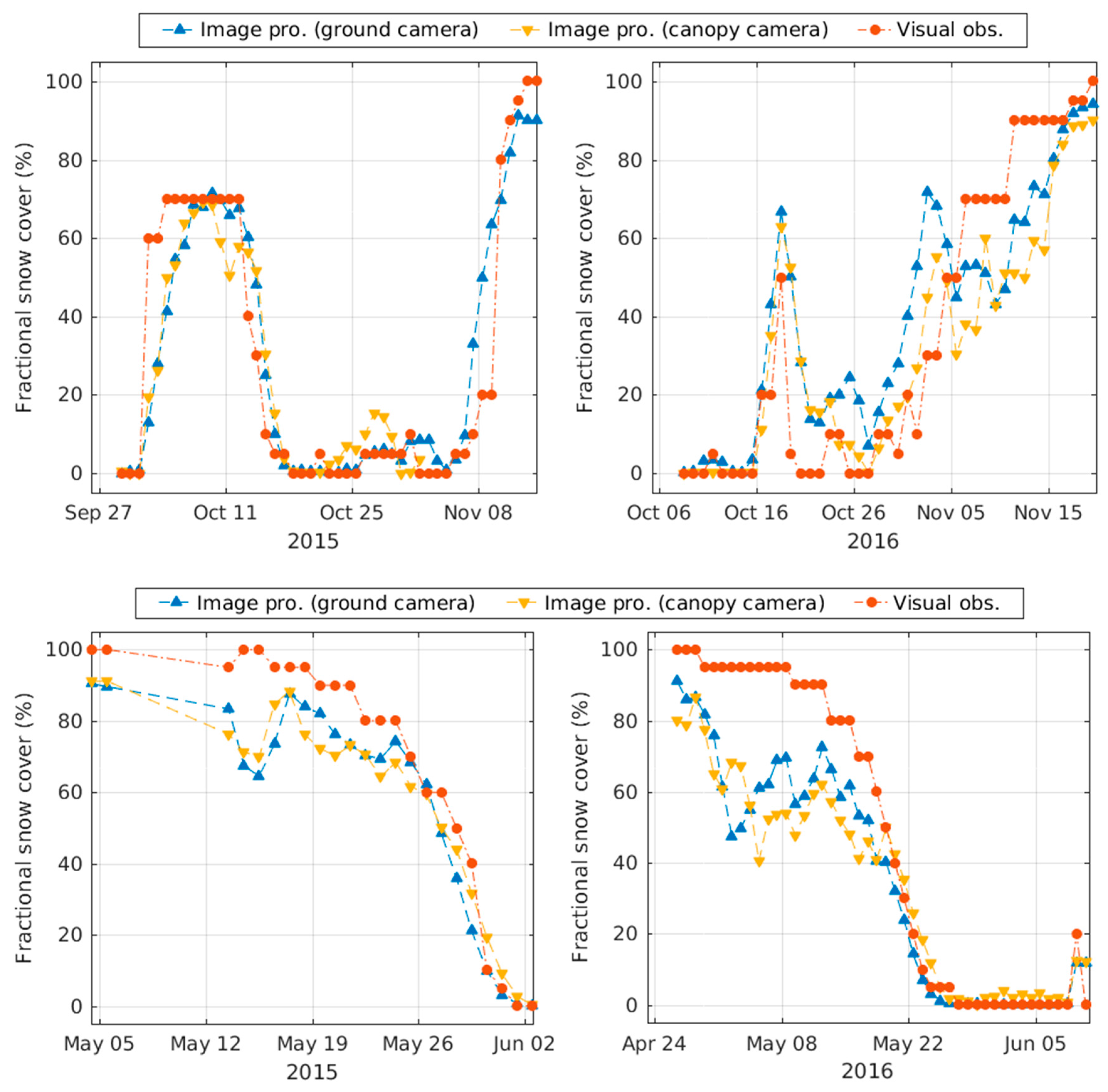
3.1. Snow Cover Analyzed as a Continuous Variable

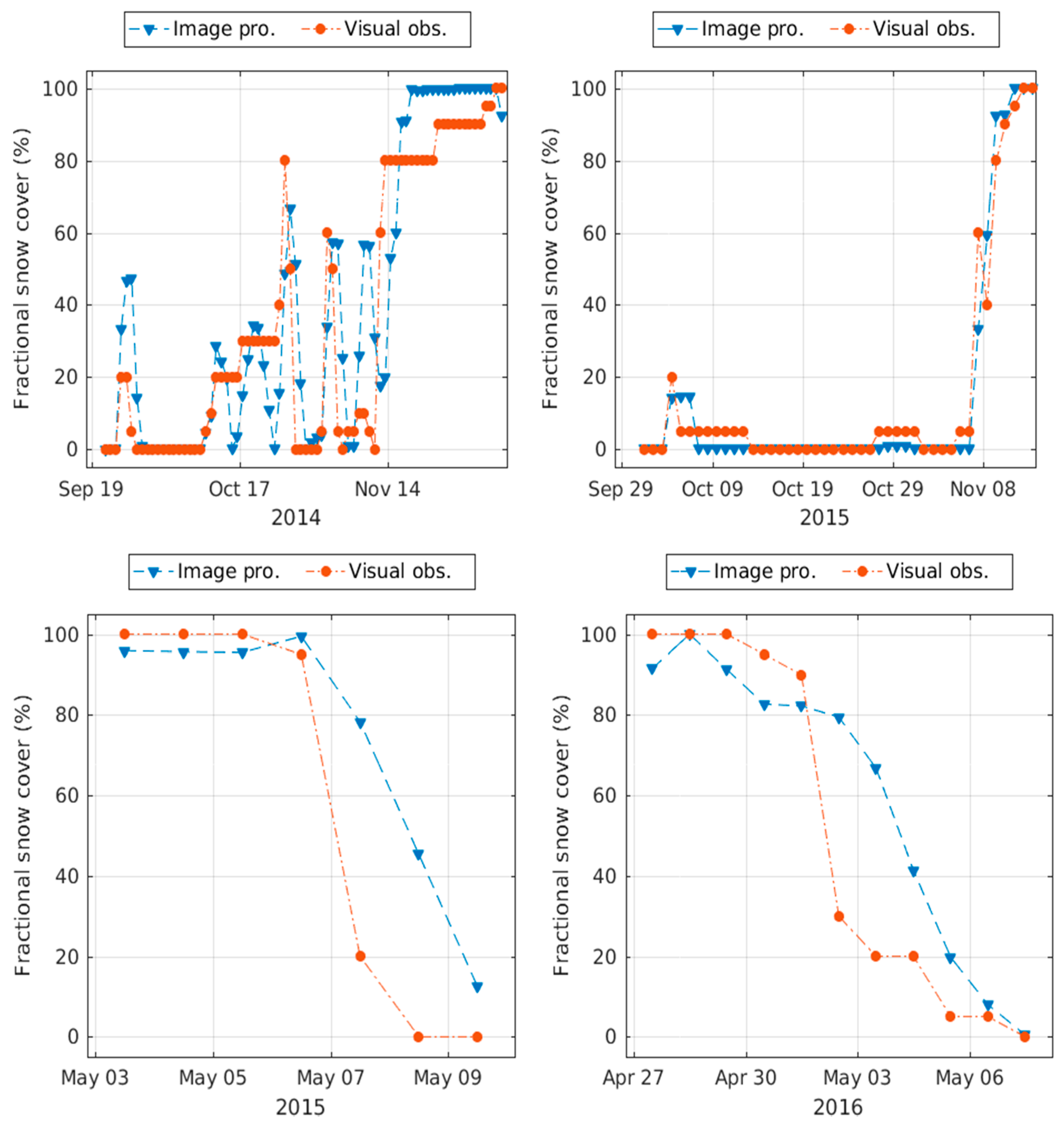
The two cameras at the Kenttärova site replicated similar FSC estimates for both early and melting seasons in 2015 and 2016 (Figure 8). Consequently, RMSE of the cameras were also very similar (
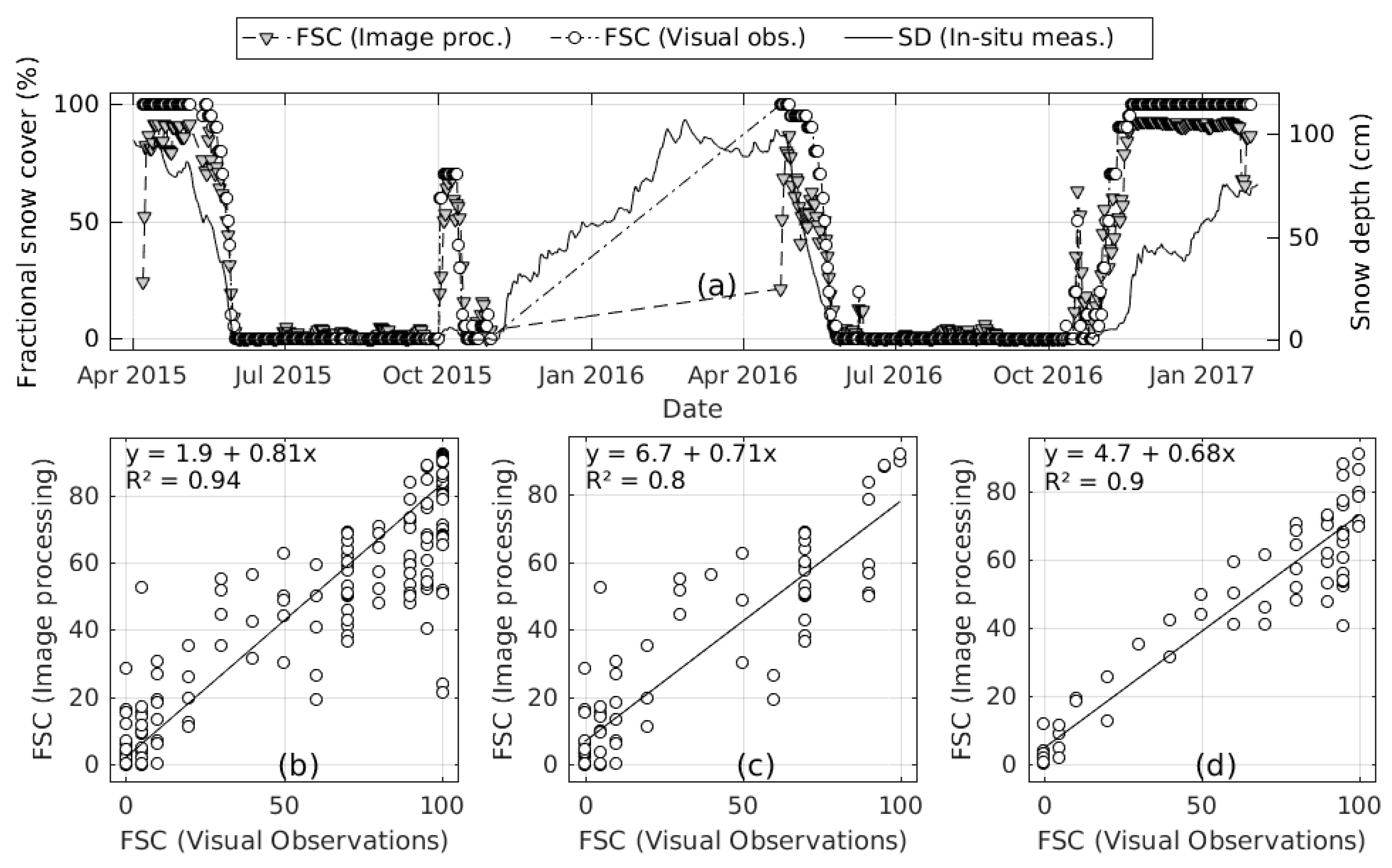
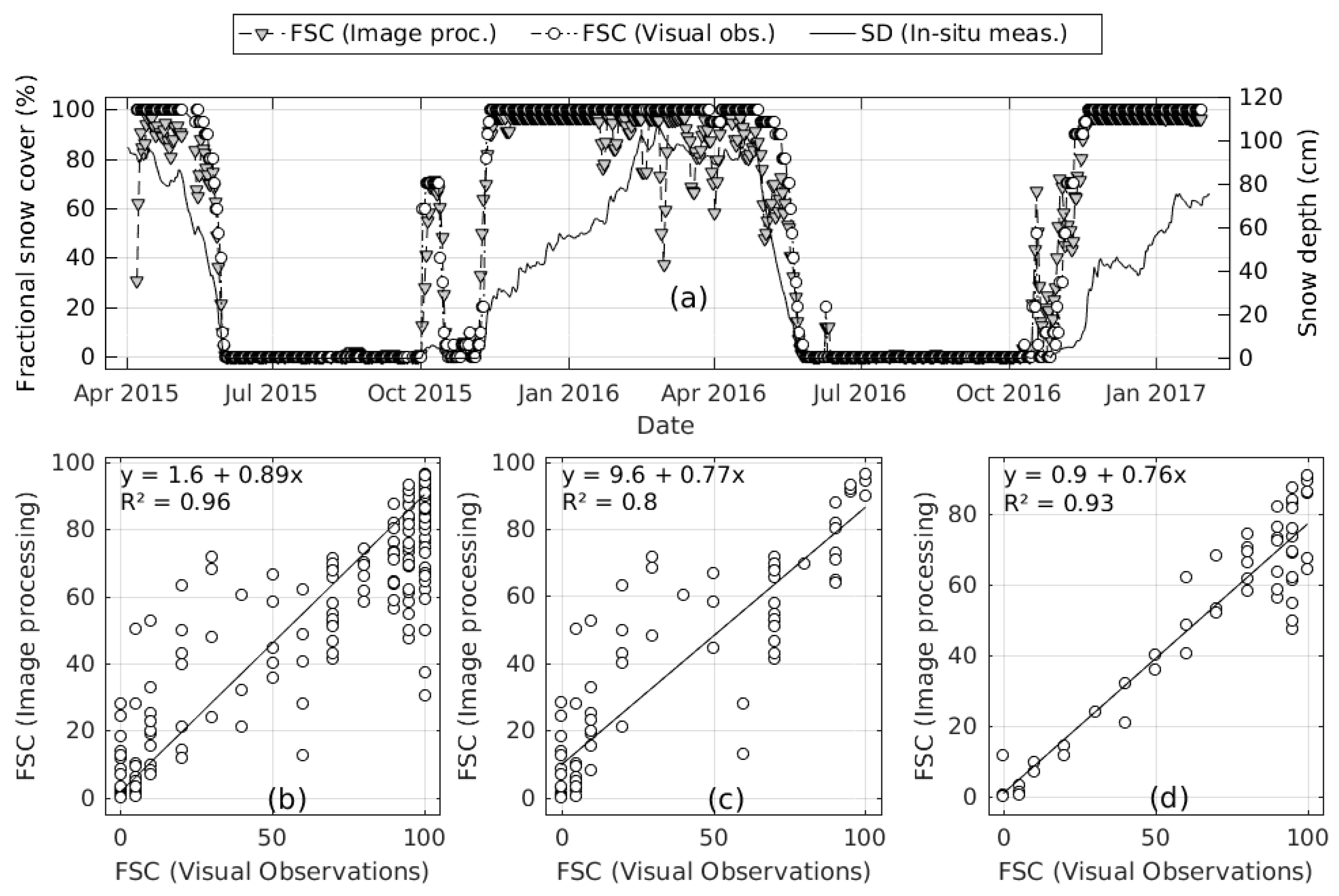
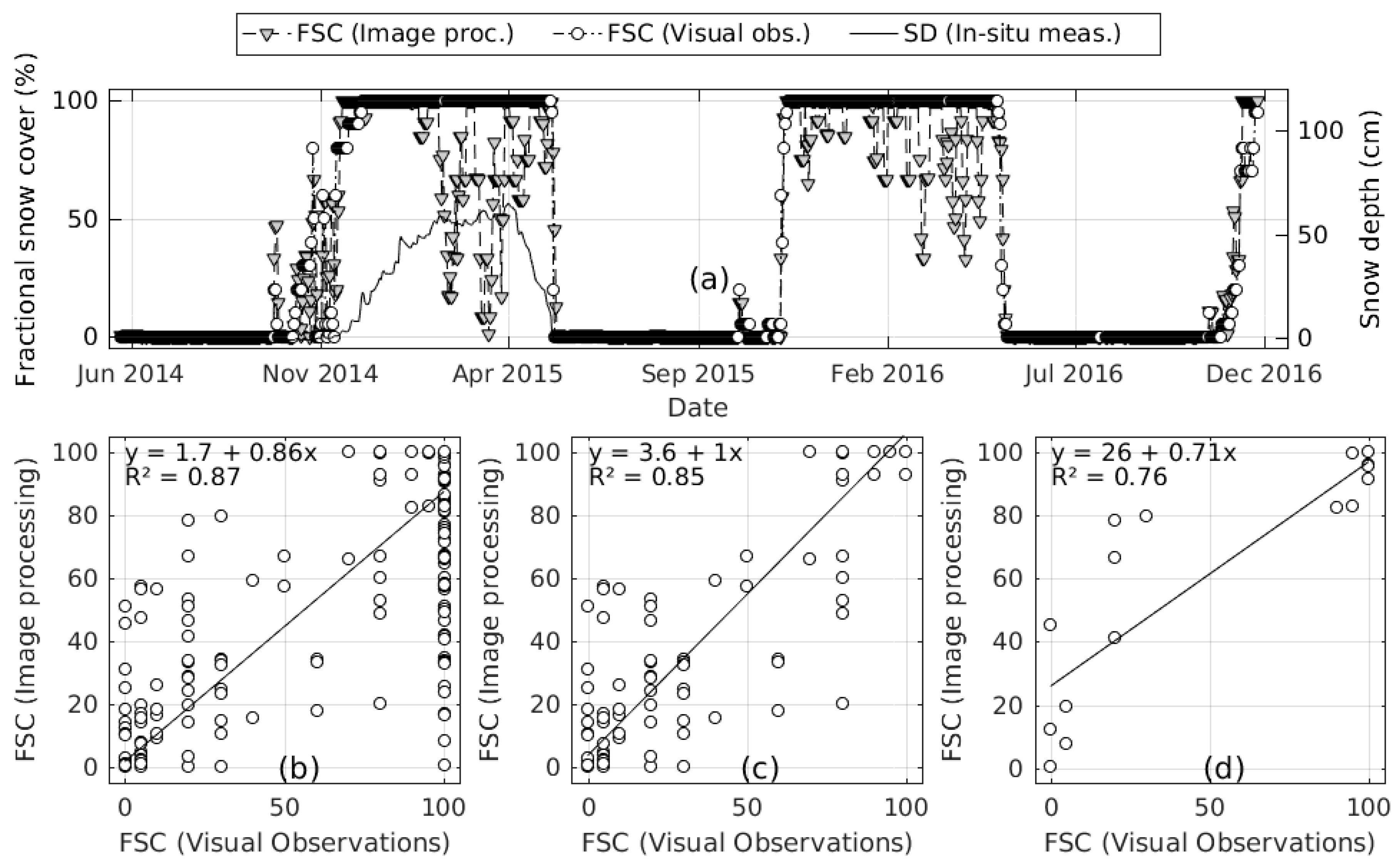
Table 4). The result also showed that FSC estimates gave good results in both early and melting seasons for both the Sodankylä ground and wetland cameras (Figure 9 and 
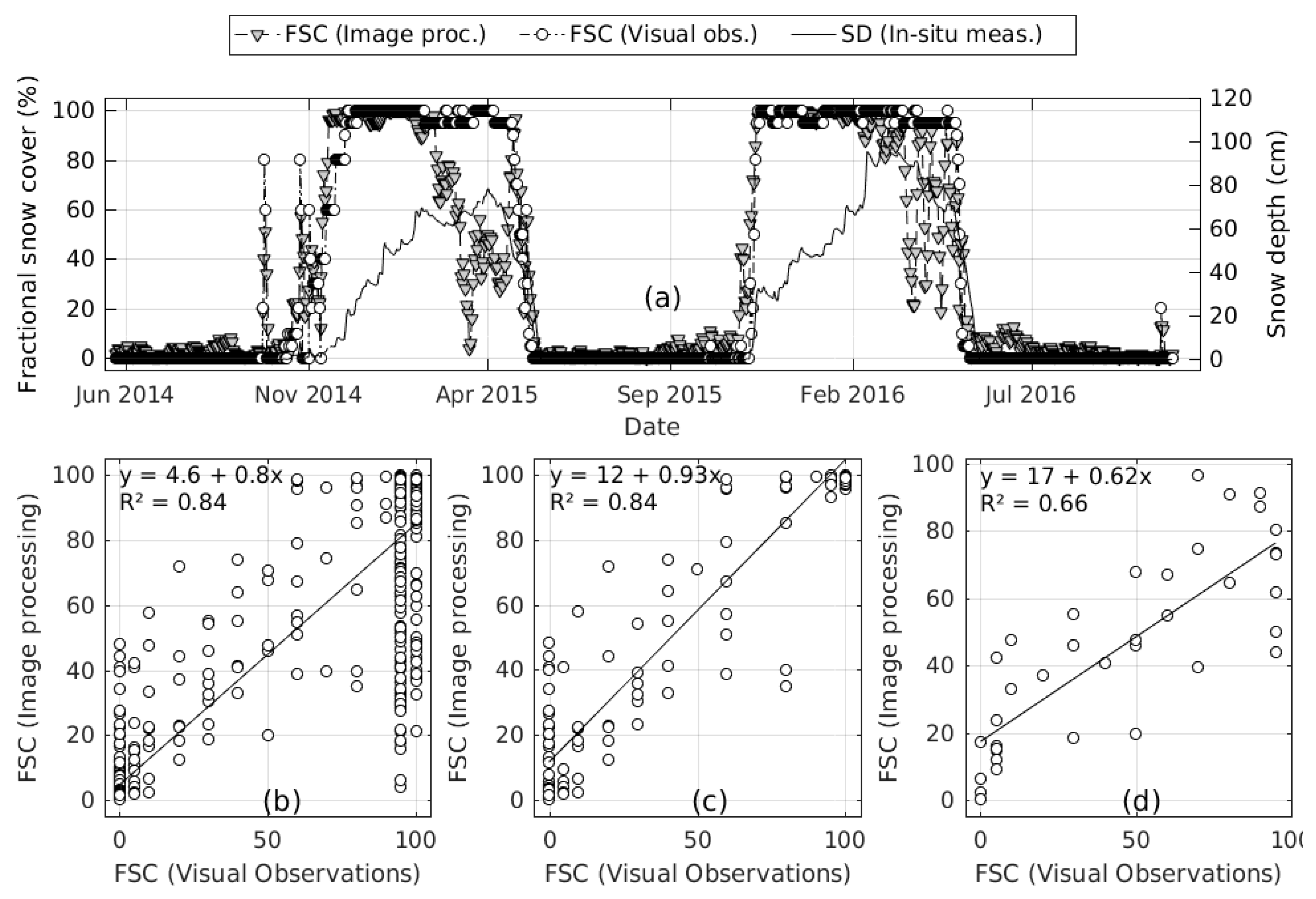
Figure 10). For all the sites, late winter results have a large number of days with high error. From the figures, it seems that these days cover a high portion of the data, but the number of days with low error are actually much more numerous throughout the year. Since the markers in the graphs are drawn on top of each other, the amount of data points is less visible (Figure 11, Figure 12, Figure 13 and Figure 14). RMSE results for seasons show that the errors of the results from the days in winters are still in a comparable range with others (Table 4). FSC estimates for all sites from image processing are in reasonably good agreement with visual observations, with R-squared values above 0.65. The slopes of all the graphs are mostly between 0.7 to 0.9, meaning the algorithm consistently underestimated the snow cover relative to the observer (Figure 11, Figure 12, Figure 13 and Figure 14).
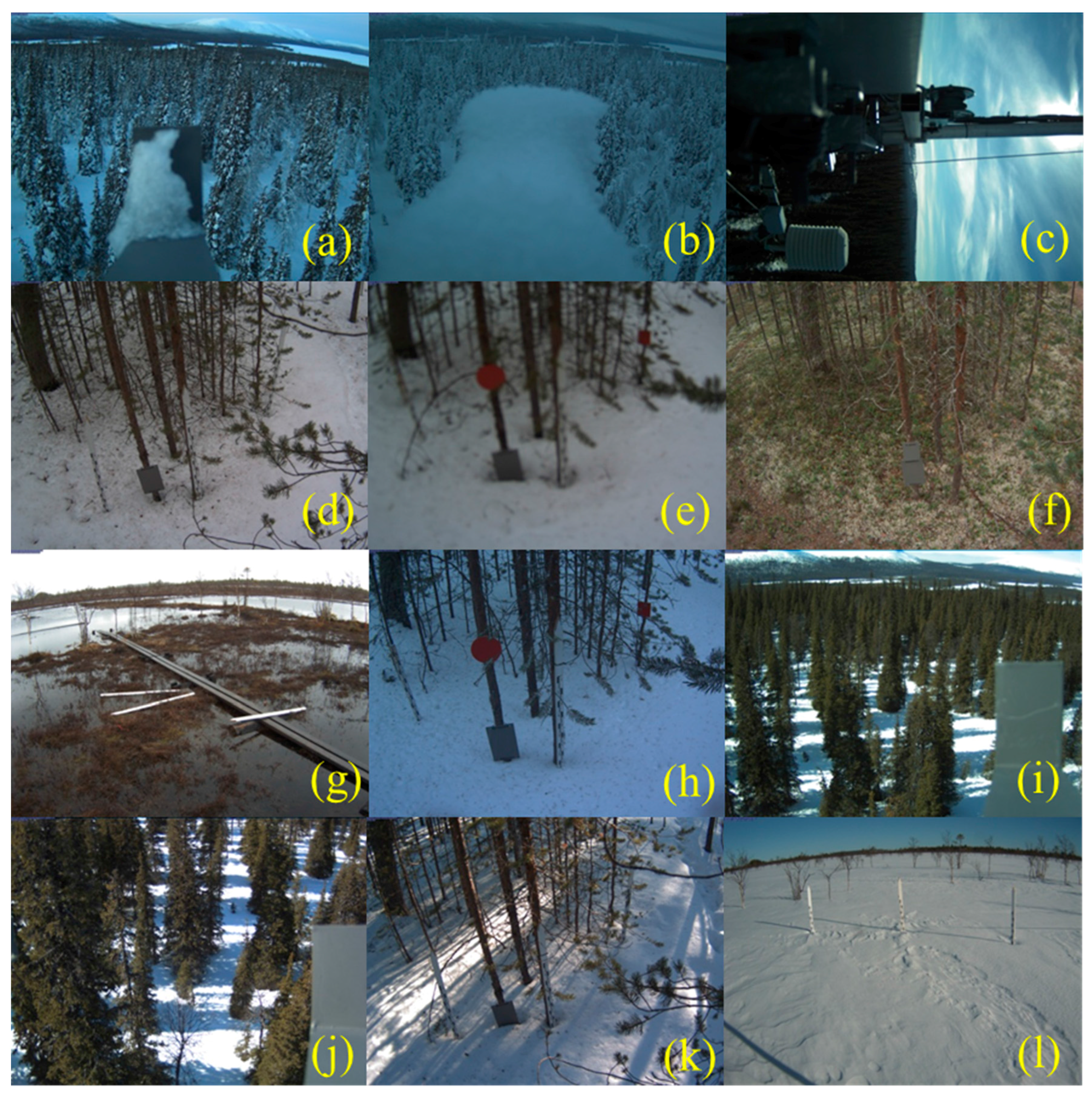
The images for which the fractional snow cover results have large error were further inspected to understand the reasons for the failure. The factors that cause failures were divided into four groups: (1) changes in the camera view, (2) environmental components that are classified as snow, (3) environmental components that hide the snow cover, and (4) phenomena that disturb the histogram. These factors occur in different circumstances, and their effects on the results are different.
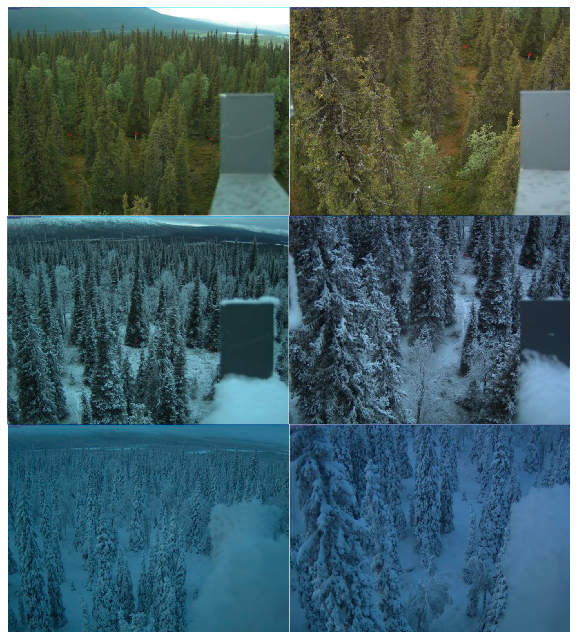
Changes in the camera view occurred on two of the four cameras. The view direction of the Kenttärova canopy camera moved to the right about 5–10 degrees in the winter of 2015–2016. The movement has not only changed the ROI, but also caused the reference plate in front of the camera to cover most of the ROI (Figure 15a). In addition, in late winter, the accumulation of the snow on the reference plate masked the field of view almost completely (Figure 15b). Later in the same winter, it is seen that the camera has moved again. The camera was also rotated 90 degrees to the right, like it has fallen down (Figure 15c). Movements on this camera change the ROI completely, thus the images from that situation were discarded from the analyses. Changes on the zoom level and focus occurred on the Sodankylä ground camera. This time, the ROI did not change as much and it covers the same area (Figure 15d,e). Thus, the images were not discarded from the analysis.
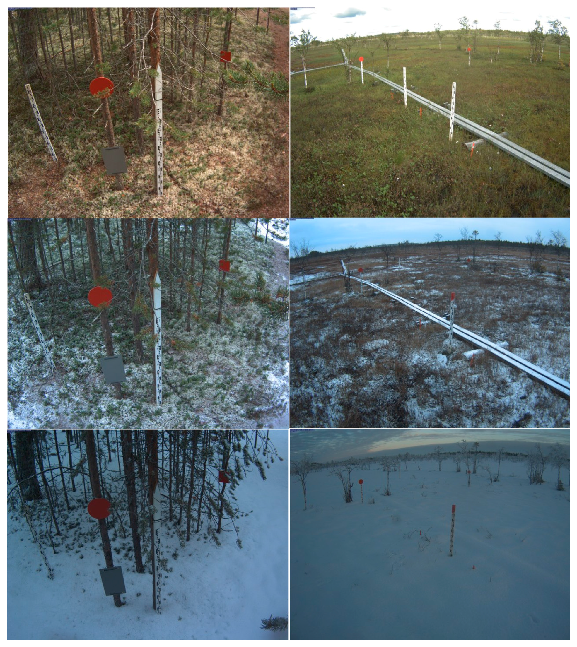
Environmental components that were classified as snow are the objects or vegetation that simply look like snow in the pixel level, even to the human eye. An example is the lichen on the ground, visible from Sodankylä ground camera in summer seasons (Figure 15f). High reflectance of lichen in the blue channel [31] near soil and green vegetation causes it to be detected as snow. Error in fractional snow cover caused by lichen is relatively low. RMSE in summer for Sodankylä is higher than other cameras, but still as low as 3.6% (Table 4). Another example is the water on the ground. High reflectance of accumulated water on bare soil in Kenttärova field of view after rain and wetland in the Sodankylä field of view in the melting season produces high values in the blue channel, depending on the direction of incoming light (Figure 15g). This effect causes the wet area to be classified as snow. Objects that had high blue channel reflectance (e.g., reference plates, snow sticks, masts, etc.) were also classified as snow (Figure 15g). Thus, such objects should not be included in ROIs, and should be stabilized so that they do not fall into ROIs when they become loose.
Environmental components that hide snow cover are objects and vegetation that block the field of view at the pixel level. The litter from trees and dirt are the most probable examples, and the effect is most visible when full snow cover is present (Figure 15h). Another example is the long branches, either from ground or trees. These branches change position due to the weight of the snow when snow accumulates on them. Even though ROIs are selected so that this situation does not disturb the analyses, some images have branches in the field of view, for example when a branch breaks and falls down on another branch.
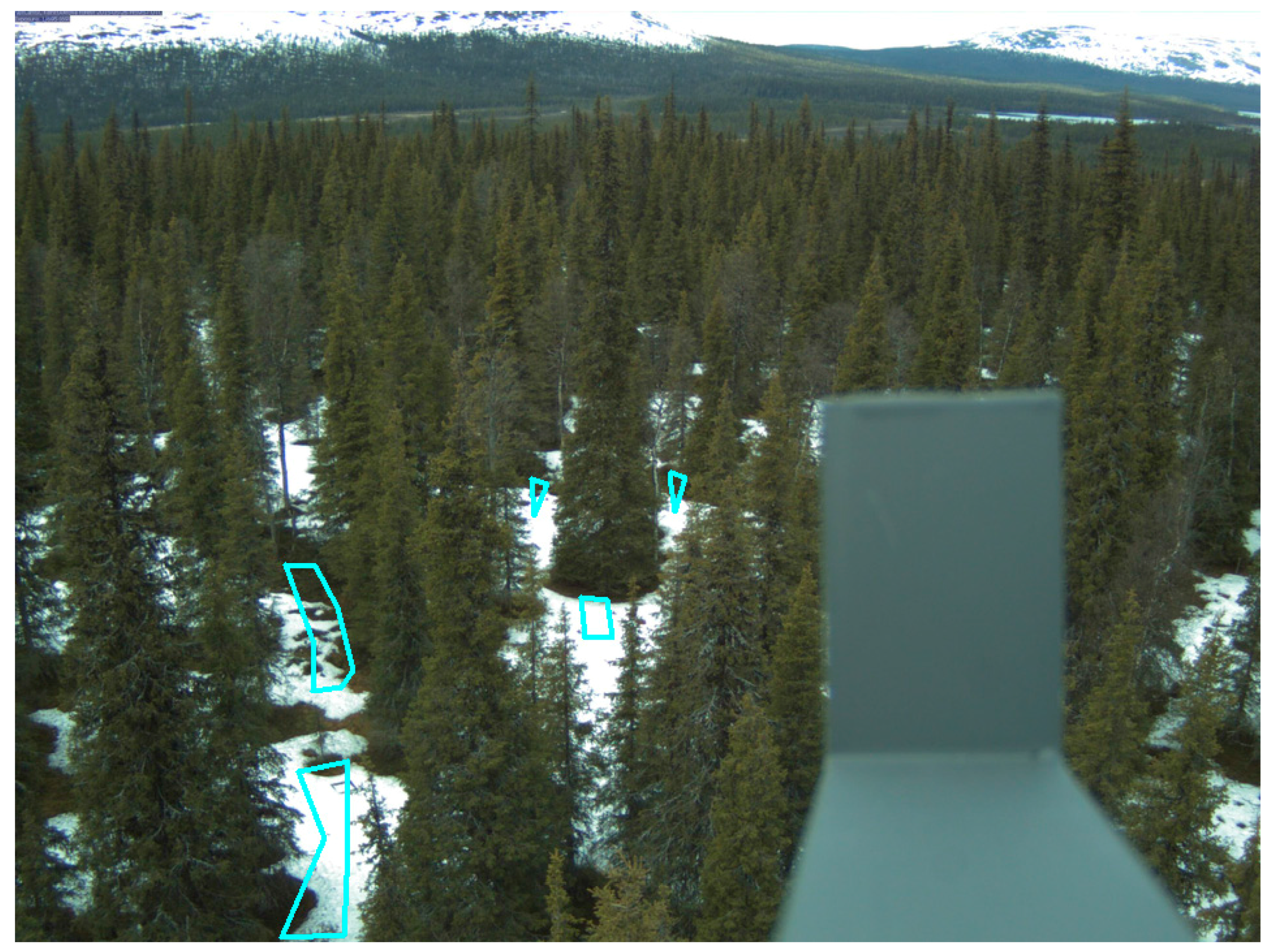
Phenomena that disturb the histogram include shades in the field of view from the objects, vegetation, clouds, and snow properties (e.g., roughness, irregularities) (
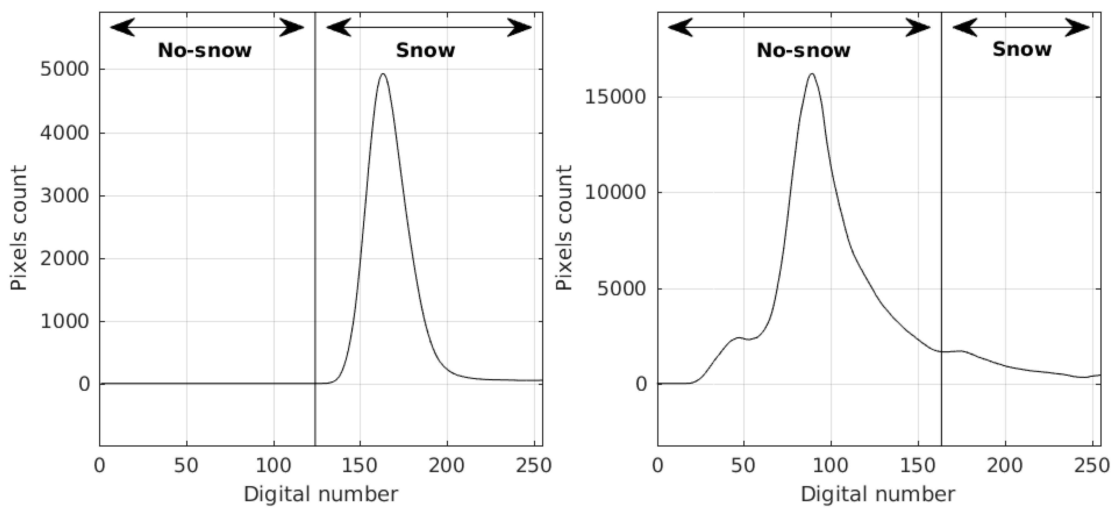
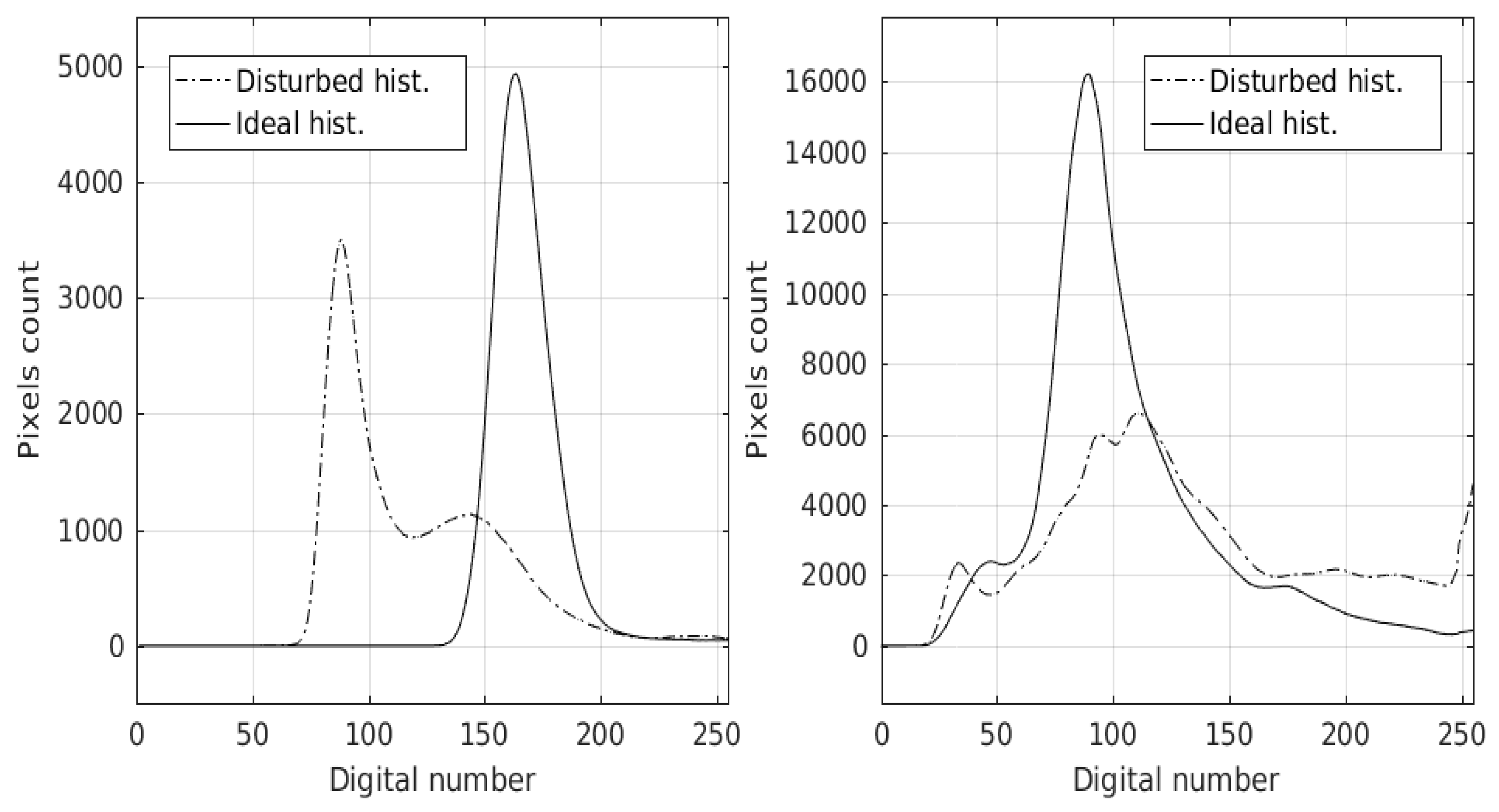
Figure 15i–l). In the situations with full cloud cover, illumination of the field of view is almost uniform. The same situation is valid when there is no cloud cover, and the ROI is selected as such that it does not include shades, either because there is no object to create a shade, or the direction of the incoming light casts the shadows in the other direction. Under uniform illumination, the histogram of the ROI can have two different signatures, as explained in the methods section. When this phenomenon occurs, different parts of the ROI have different levels of illumination. Parts in shadow are much darker than the others. That causes the number of distribution components (peaks) to be doubled (Figure 16). In that case, the automatic selection of threshold by the algorithm causes the shady areas to be classifed as snow-free and non-shady areas to be classified as snow-covered, regardless of whether the pixels correponded to snow cover. The error caused by this phenomenon can be up to 99%. This phenomenon is observed in almost all the images with an error larger than 50%.
Histogram disturbing by shade phenomenon is the most significant failure, as it causes the largest errors. Besides, failures by environmental components occurred mostly in summer, and can be discarded from the analyses or studies. Changes in camera view are also easier to spot because they generally cover an interval of time. But the shade phenomenon depends on the cloud cover, environment and sunlight direction, and this may change even within minutes. Thus, one should inspect all the images and list them in order to discard problematic ones, but such intervention would be further away to the idea of automatized processing, and also would mean losing a large amount of data. Instead, the algorithm should be developed or trained with the information about histograms under different light conditions, possibly by supervising the algorithm training with visual inspection and classification of sun/shade images.

3.2. Categorical Snow Cover Analysis

We prepared confusion matrices with accuracies and errors for all four selected regions (Table 5, Table 6, Table 7 and Table 8).The producer accuracy was highest in Class A (0–10%), around 0.92, and reasonably good in other Classes (B: 10–50, C, 50–90; D: 90–100), between 0.6 and 0.7 for all sites, except Class C, 0.21 and 0.32 in Sodankylä wetland and ground sites, respectively.

4. Conclusions

Estimation of fractional snow cover (FSC) is critical to water management, and important for meteorological, climatological, and hydrological applications. Retrieving of FSC, particularly over forested areas by satellite remote sensing, is challenging; furthermore, the development and validation of new algorithms, along with the new generation satellite sensors, sets a need for good quality data validation. However, both in situ FSC, and high resolution satellite data-based reference snow maps for the evaluation of moderate resolution FSC retrievals, are difficult to obtain. Particularly, no properly working algorithms for creating an accurate high resolution FSC reference maps for boreal forests are available. Our earlier studies show that validation results using high resolution FSC-maps as reference may give substantially different results, depending on the applied FSC-algorithm [14].
Due to the above-mentioned problems, we have applied a technique for retrieving temporally very frequent information on the local site-specific FSC, using a network of digital cameras. Based on our results, we conclude that snow cover could be analyzed with consumer grade cameras. The results showed that the tested snow algorithm is able to estimate fractional snow cover with high R-squared and low RMSE values. The gained RMSEs varied between 12% and 30% (FSC %-units), excluding the summer season, as it provided very low RMSEs, due to lack of snow. We analyzed the reasons for large estimation errors in the automatic snow cover classification in particular cases. The main error source was the occurrence of shaded areas in the region of interest. We showed that cameras could be used to monitor snow status with reasonable accuracy, and could thus be used to improve FSC retrieval algorithms from remote sensing data and/or to validate Earth-observed FSC. Therefore, camera-based algorithms should be further developed, especially for varying light conditions in the field of view, to obtain better accuracy in FSC retrieval. Another way of obtaining better accuracy in FSC retrieval, is to implement a balanced enhancement technique for improving the visual quality of both highlights and dark areas [32,33].

Acknowledgments

The work was funded by European Commission through EU Life+ project MONIMET Project (LIFE12ENV/FI/000409) during 2013–2017. We thank Juuso Rainne (FMI) for installing and maintaining the cameras. Esa Ek (LUKE) is acknowledged for making visual observations.

Author Contributions

A.N.A. and C.M.T. designed the study and implemented snow algorithm and conducted snow analyses, S.M. first inspired the way the accuracy analysis was made and also contributed in the considerations of satellite FSC retrievals, M.A., K.B., C.M.T., M.L. and M.P. worked on planning the camera set-up and installation of all the cameras, M.P. provided visual observation and A.N.A. and C.M.T. wrote the paper and others contributed to the text.

Conflicts of Interest

The authors declare no conflict of interest.

References

  1. Matikainen, L.; Kuittinen, R.; Vepsäläinen, J. Estimating drainage area-based snow cover percentages from NOAA/AVHRR images. Int. J. Remote Sens. 2002, 23, 2971–2988. [Google Scholar] [CrossRef]
  2. Metsämäki, S.; Vepsäläinen, J.; Pulliainen, J.; Sucksdorff, Y. Improved linear interpolation method for the estimation of snow-covered area from optical data. Remote Sens Environ. 2002, 82, 64–78. [Google Scholar] [CrossRef]
  3. Painter, T.H.; Dozier, J.; Roberts, D.A.; Davis, R.E.; Green, R.O. Retrieval of subpixel snow-covered area and grain size from imaging spectrometer data. Remote Sens Environ. 2003, 85, 64–77. [Google Scholar] [CrossRef]
  4. Salomonson, V.V.; Appel, I. Estimating fractional snow cover from MODIS using the normalized difference snow index. Remote Sens. Environ. 2004, 89, 351–360. [Google Scholar] [CrossRef]
  5. Salomonson, V.V.; Appel, I. Development of the Aqua MODIS NDSI fractional snow cover algorithm and validation results. IEEE Trans. Geosci. Remote Sens. 2006, 44, 1747–1756. [Google Scholar] [CrossRef]
  6. Painter, T.H.; Rittger, K.; McKenzie, C.; Slaughter, P.; Davis, R.E.; Dozier, J. Retrieval of subpixel snow covered area, grain size, and albedo from MODIS. Remote Sens Environ. 2009, 113, 868–879. [Google Scholar] [CrossRef]
  7. Dozier, J.; Green, R.O.; Nolin, A.W.; Painter, T.H. Interpretation of snow properties from imaging spectrometry. Remote Sens. Environ. 2009, 113, s25–s37. [Google Scholar] [CrossRef]
  8. Klein, A.G.; Hall, D.K.; Riggs, G.A. Improving snow-cover mapping in forests through the use of a canopy reflectance model. Hydrol. Process. 1998, 12, 1723–1744. [Google Scholar] [CrossRef]
  9. Vikhamar, D.; Solberg, R. Subpixel mapping of snow cover in forests by optical remote sensing. Remote Sens Environ. 2003, 84, 69–82. [Google Scholar] [CrossRef]
  10. Hall, D.K.; Riggs, G.A. Accuracy assessment of the MODIS snow products. Hydrol. Process. 2007, 21, 1534–1547. [Google Scholar] [CrossRef]
  11. Rittger, K.; Painter, T.H.; Dozier, J. Assessment of methods for mapping snow cover from MODIS. Adv. Water Resour. 2012, 51, 367–380. [Google Scholar] [CrossRef]
  12. Metsämäki, S.; Mattila, O.P.; Pulliainen, J.; Niemi, K.; Luojus, K.; Böttcher, K. An optical reflectance model-based method for fractional snow cover mapping applicable to continental scale. Remote Sens. Environ. 2012, 123, 508–521. [Google Scholar] [CrossRef]
  13. Wang, X.Y.; Wang, J.; Jiang, Z.Y.; Li, H.Y.; Hao, X.H. An effective method for snow-cover mapping of dense coniferous forests in the upper Heihe river basin using Landsat operational land imager data. Remote Sens. 2015, 7, 17246–17257. [Google Scholar] [CrossRef]
  14. Metsämäki, S.; Pulliainen, J.; Salminen, M.; Luojus, K.; Wiesmann, A.; Solberg, R.; Böttcher, K.; Hiltunen, M.; Ripper, E. Introduction to GlobSnow Snow Extent products with considerations for accuracy assessment. Remote Sens. Environ. 2015, 156, 96–108. [Google Scholar] [CrossRef]
  15. Wingate, L.; Ogée, J.; Cremonese, E.; Filippa, G.; Mizunuma, T.; Migliavacca, M.; Moisy, C.; Wilkinson, M.; Moureaux, C.; Wohlfahrt, G.; et al. Interpreting canopy development and physiology using a European phenology camera network at flux sites. Biogeosciences 2015, 12, 5995–6015. [Google Scholar] [CrossRef]
  16. Phenocam. Available online: https://phenocam.sr.unh.edu/webcam/ (accessed on 19 August 2016).
  17. Australian Phenocam Network. Available online: https://phenocam.org.au/ (accessed on 19 August 2016).
  18. Tsuchida, S.; Nishida, K.; Kawato, W.; Oguma, H.; Iwasaki, A. Phenological eyes network for validation of remote sensing data. J. Remote Sens. Soc. Jpn. 2005, 25, 282–288. [Google Scholar]
  19. Peltoniemi, M.; Böttcher, K.; Aurela, M.; Kolari, P.; Tanis, C.M.; Linkosalmi, M.; Loehr, J.; Metsämäki, S.; Arslan, A.N. Phenology cameras observing boreal ecosystems of Finland. In Proceedings of the European Geosciences Union General Assembly Conference, Vienna, Austria, 17–22 April 2016; Volume 18, p. 17185. [Google Scholar]
  20. Ide, R.; Oguma, H. Use of digital cameras for phenological observations. Ecol. Inform. 2010, 5, 339–347. [Google Scholar] [CrossRef]
  21. Filippa, G.; Cremonese, E.; Migliavacca, M.; Galvagno, M.; Forkel, M.; Wingate, L.; Tomelleri, E.; Morra di Cella, U.; Richardson, A.D. Phenopix: A R package for image-based vegetation phenology. Agric. For. Meteorol. 2016, 220, 141–150. [Google Scholar] [CrossRef]
  22. Linkosalmi, M.; Aurela, M.; Tuovinen, J.-P.; Peltoniemi, M.; Tanis, C.M.; Arslan, A.N.; Kolari, P.; Aalto, T.; Rainne, J.; Laurila, T. Digital photography for assessing vegetation phenology in two contrasting northern ecosystems. Geosci. Instrum. Methods Data Syst. 2016, 5, 417–426. [Google Scholar] [CrossRef]
  23. Bernard, E.; Friedt, J.M.; Tolle, F.; Griselin, M.; Martin, G.; Laffly, D.; Marlin, C. Monitoring seasonal snow dynamics using ground based high resolution photography (Austre Lovénbreen, Svalbard, 79°N). ISPRS J. Photogramm. Remote Sens. 2013, 75, 92–100. [Google Scholar] [CrossRef]
  24. Garvelmann, J.; Pohl, S.; Weiler, M. From observation to the quantification of snow processes with a time-lapse camera network. Hydrol. Earth Syst. Sci. 2013, 17, 1415–1429. [Google Scholar] [CrossRef]
  25. Härer, S.; Bernhardt, M.; Corripio, J.G.; Schulz, K. PRACTISE—Photo Rectification and ClassificaTIon SoftwarE (V.1.0). Geosci. Model Dev. 2013, 6, 837–848. [Google Scholar] [CrossRef]
  26. Salvatori, R.; Plini, P.; Giusto, M.; Valt, M.; Salzano, R.; Montagnoli, M.; Cagnati, A.; Crepaz, G.; Sigismondi, D. Snow cover monitoring with images from digital camera systems. Ital. J. Remote Sens. 2011, 137–145. [Google Scholar] [CrossRef]
  27. Wang, J.; Robinson, G.J.; White, K. Generating viewsheds without using sightlines. Photogramm. Eng. Remote Sens. 2000, 66, 87–90. [Google Scholar]
  28. Heikkila, J.; Silven, O. A four-step camera calibration procedure with implicit image correction. In Proceedings of the IEEE Computer Society Conference on Computer Vision and Pattern Recognition, San Juan, Puerto Rico, 17–19 June 1997; pp. 1106–1112. [Google Scholar]
  29. Corripio, J.G. Snow surface albedo estimation using terrestrial photography. Int. J. Remote Sens. 2004, 25, 5705–5729. [Google Scholar] [CrossRef]
  30. Monimet. Available online: http://monimet.fmi.fi?page=FMIPROT (accessed on 1 January 2014).
  31. Rees, W.; Tutubalina, O.; Golubeva, E. Reflectance spectra of subarctic lichens between 400 and 2400 nm. Remote Sens. Environ. 2004, 90, 281–292. [Google Scholar] [CrossRef]
  32. Wang, Y.; Luo, Y. Balanced color contrast enhancement for digital images. Opt. Eng. 2012, 51, 1–11. [Google Scholar] [CrossRef]
  33. Wang, S.; Zheng, J.; Hu, H.M.; Li, B. Naturalness preserved enhancement algorithm for non-uniform illumination images. IEEE Trans. Image Process. 2013, 22, 3538–3548. [Google Scholar] [CrossRef] [PubMed]
Figure 1. Example images from canopy (left panels) and ground cameras (right panels) of Kenttärova on 18 June 2016, 12:00 (top), 3 November 2016, 09:30 (center) and 25 November 2016, 11:00 (bottom).
Geosciences 07 00055 g001
Figure 2. Example images in both summer and winter conditions from ground (left panels) and wetland cameras (right panels) of Sodankylä on 18 June 2016, 12:01 (top), 3 November 2016, 09:31 (center) and 25 November 2016, 11:01 (bottom).
Geosciences 07 00055 g002
Figure 3. Sodankylä wetland camera region of interest (ROI).
Geosciences 07 00055 g003
Figure 4. Kenttärova canopy camera ROI.
Geosciences 07 00055 g004
Figure 5. Camera orientation parameters defining the viewing geometry.
Geosciences 07 00055 g005
Figure 6. Threshold selection for snow classification for two different types of histogram distributions. The histograms are extracted from real images and smoothed in the same way in the algorithm.
Geosciences 07 00055 g006
Figure 7. Main steps of calculating fractional snow cover for a single image: (a) Original image; (b) Corresponding y coordinates of the image on the spatial grid; (c) Corresponding x coordinates of the image on the spatial grid; (d) Georeferenced image on the spatial grid (for (bd), spatial area is cropped according to the ROI.); (e) The mask to be applied for the ROI; (f) Snow-covered and snow-free pixels in ROI; and (g) Weight of the surface area for each pixel in the ROI.
Geosciences 07 00055 g007
Figure 8. Kenttärova ground and canopy cameras early season (top) and melting season (bottom); comparisons of image processing results and visual observations.
Geosciences 07 00055 g008
Figure 9. Sodankylä ground camera early season (top) and melting season (bottom); comparisons of image processing results and visual observations.
Geosciences 07 00055 g009
Figure 10. Sodankylä wetland camera early season (top) and melting season (bottom) comparison of image processing results and visual observations.
Geosciences 07 00055 g010
Figure 11. Kenttärova canopy camera: (a) 3-day moving window averaged fractional snow cover over time from image processing and daily visual observations, daily averaged snow depth over time from automatic ground measurements. Distribution and regression of fractional snow cover from image processing versus visual observations for (b) all data; (c) early season; and (d) melting season.
Geosciences 07 00055 g011
Figure 12. Kenttärova ground camera: (a) 3-day moving window averaged fractional snow cover over time from image processing and daily visual observations, daily averaged snow depth over time from automatic ground measurements. Distribution and regression of fractional snow cover from image processing versus visual observations for (b) all data; (c) early season; and (d) melting season.
Geosciences 07 00055 g012
Figure 13. Sodankylä wetland camera: (a) 3-day moving window averaged fractional snow cover over time from image processing and daily visual observations, daily averaged snow depth over time from automatic ground measurements. Distribution and regression of fractional snow cover from image processing versus visual observations for (b) all data; (c) early season; and (d) melting season.
Geosciences 07 00055 g013
Figure 14. Sodankylä ground camera: (a) 3-day moving window averaged fractional snow cover over time from image processing and daily visual observations, daily averaged snow depth over time from automatic ground measurements. Distribution and regression of fractional snow cover from image processing versus visual observations for (b) all data; (c) early season; and (d) melting season.
Geosciences 07 00055 g014
Figure 15. Problems in the images that cause failures in detection of fractional snow cover: (a) Field of view blocked by the reference plate after the camera movement; (b) Field of view blocked by the accumulation of snow on reference plate; (c) Field of view loss after the camera movement; (d,e) Before and after the minimal camera movement and loss of focus; (f) Lichen on the ground; (g) Water accumulation which reflects the bright sky and fallen snow sticks; (h) Litter and dirt on the ground; (i) Shadow of trees in Kenttärova canopy camera field of view; (j) Shadow of trees in Kenttärova ground camera field of view; (k) Shadow by trees and snow sticks in Sodankylä ground camera field of view; (l) Shadow by the snow surface irregularites, snow roughness, snow sticks, and camera mast.
Geosciences 07 00055 g015
Figure 16. Examples of histogram disturbance by shade. Ideal histogram and disturbed histogram (left) for full snow cover and (right) for partial snow cover.
Geosciences 07 00055 g016
Table 1. Orthorectification parameters for the cameras.
Camera NameLongitude (Camera X)Latitude (Camera Y)Height (Camera Z)Geographic Direction Angle (Yaw)Vertical Angle (Pitch)Horizontal Angle (Roll)Focal LengthScaling Factor
Sodankylä Ground26.63751°67.36201°2.46 m96°34°−1°4 mm187,500
Sodankylä Wetland26.65442°67.36849°2.08 m25°18°4 mm8,3131
Kenttärova Canopy24.24302°67.98726°21.20 m273°20°−1°4 mm2,214,048
Kenttärova Ground24.24302°67.98726°21.28 m247°35°4 mm1,190,033
Table 2. Definition of Seasons.
Site/Year201420152016
Early Season
Kenttärova 29 September–15 November 20158 October–21 November 2016
Sodankylä wetland21 September–6 December 20141 October–14 November 201514. October–28 November 2016
Sodankylä ground21 September–15 December 201424 October–18 November 201514. October–30 October 2016
Melting Season
Kenttärova 5 April–3 May 201526 April–12 June 2016
Sodankylä wetland 3 May–10 May 201527 April–9 May 2016
Sodankylä ground 19 April–10 May 201525 April–11 May 2016
Winter SeasonBetween early seasonand melting season
Summer SeasonAfter melting season
Table 3. Confusion matrices.
Estimated/ReferenceClass AClass BClass CClass DUser’s AccuracyCommission Error
Class A n A A n B A n C A n D A a c c U A e r r C A
Class B n A B n B B n C B n D B a c c U B e r r C B
Class C n A C n B C n C C n D C a c c U C e r r C C
Class D n A D n B D n C D n D D a c c U D e r r C D
Producer’s Accuracy a c c P A a c c P B a c c P C a c c P D
Omission Error e r r O A e r r O B e r r O C e r r O D
Table 4. RMSE for the fractional snow cover (FSC) from image processing for all seasons.
Season/SiteKenttärova CanopyKenttärova GroundSodankylä GroundSodankylä Wetland
Early Season16171816
Mid-winter18123027
Melting Season20182124
Summer1.70.453.60.27
Overall13111918
Overall except summer18142624
Table 5. Confusion matrices for Kenttärova canopy camera.
Estimated/ReferenceClass A (0–10)Class B (10–50)Class C (50–90)Class D (90–100)User’s AccuracyCommission Error
Class A2770001.000.00
Class B1691450.200.80
Class C1319550.240.76
Class D000781.000.00
Producer’s Accuracy0.940.750.580.57
Omission Error0.060.250.420.43
Total Accuracy: 0.80Total Error: 0.20
Table 6. Confusion matrices for Kenttärova ground camera.
Estimated/ReferenceClass A (0–10)Class B (10–50)Class C (50–90)Class D (90–100)User’s AccuracyCommission Error
Class A2810001.000.00
Class B15101050.250.75
Class C2424840.210.79
Class D0002121.000.00
Producer’s Accuracy0.940.710.710.70
Omission Error0.060.290.290.30
Total Accuracy: 0.81Total Error: 0.19
Table 7. Confusion matrices for Sodankylä ground camera.
Estimated/ReferenceClass A (0–10)Class B (10–50)Class C (50–90)Class D (90–100)User’s AccuracyCommission Error
Class A4810021.000.00
Class B39167520.140.86
Class C1611660.130.87
Class D00161910.920.08
Producer’s Accuracy0.920.730.320.61
Omission Error0.080.270.680.39
Total Accuracy: 0.79Total Error: 0.21
Table 8. Confusion matrices for Sodankylä wetland camera.
Estimated/ReferenceClass A (0–10)Class B (10–50)Class C (50–90)Class D (90–100)User’s AccuracyCommission Error
Class A4933050.980.02
Class B19185230.280.72
Class C466900.060.94
Class D00182210.920.08
Producer’s Accuracy0.960.670.210.65
Omission Error0.040.330.790.35
Total Accuracy: 0.81Total Error: 0.19

