
Natural Sinkhole Monitoring and Characterization: The Case of Latera Sinkhole (Latium, Central Italy)

 , ,
, ,  and
and
Abstract
:1. Introduction
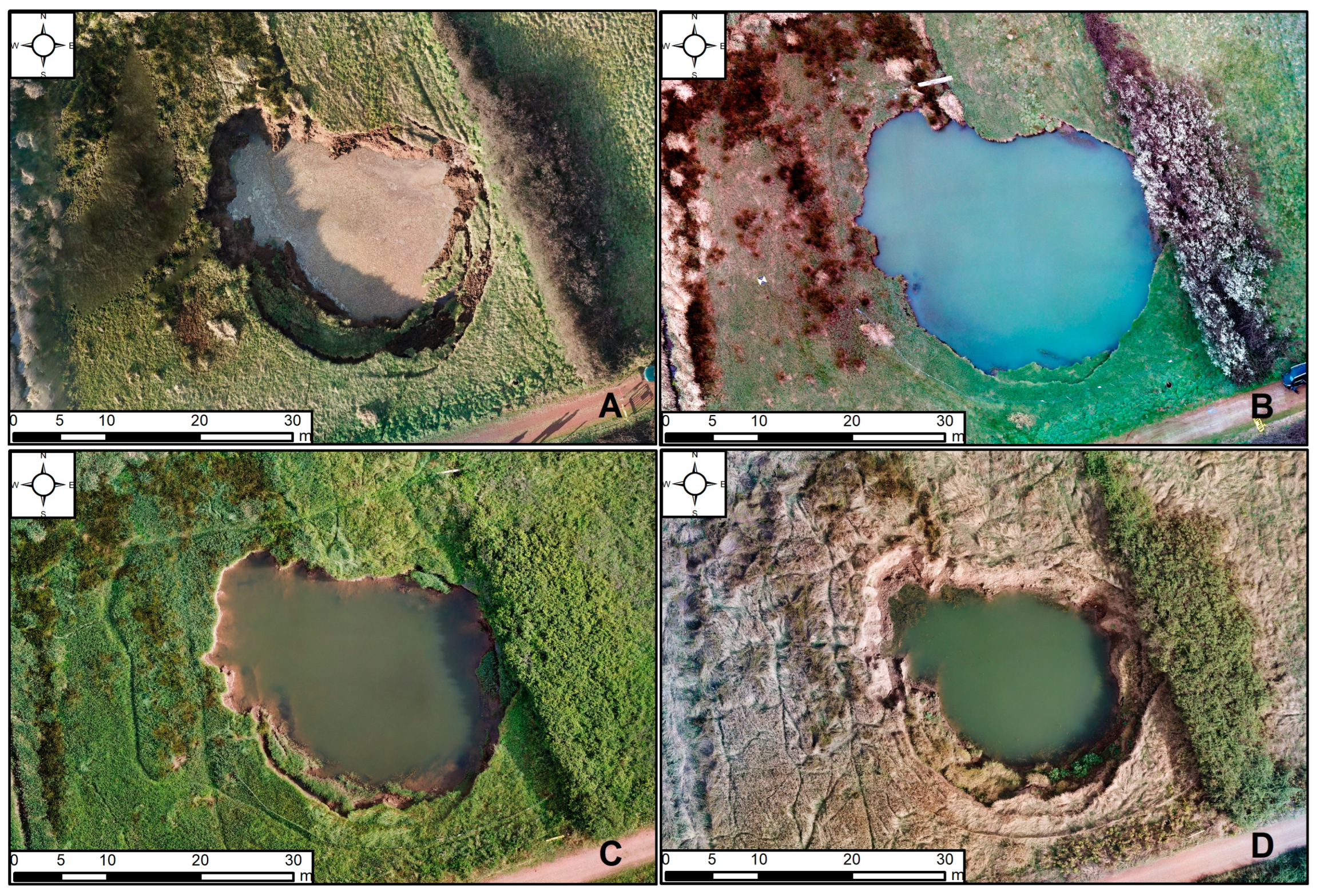
- Monthly based monitoring by using an Uncrewed Aerial Vehicle (UAV) to evaluate soil subsidence and study the rise in the groundwater level in the collapse during the first 30 days after its formation.
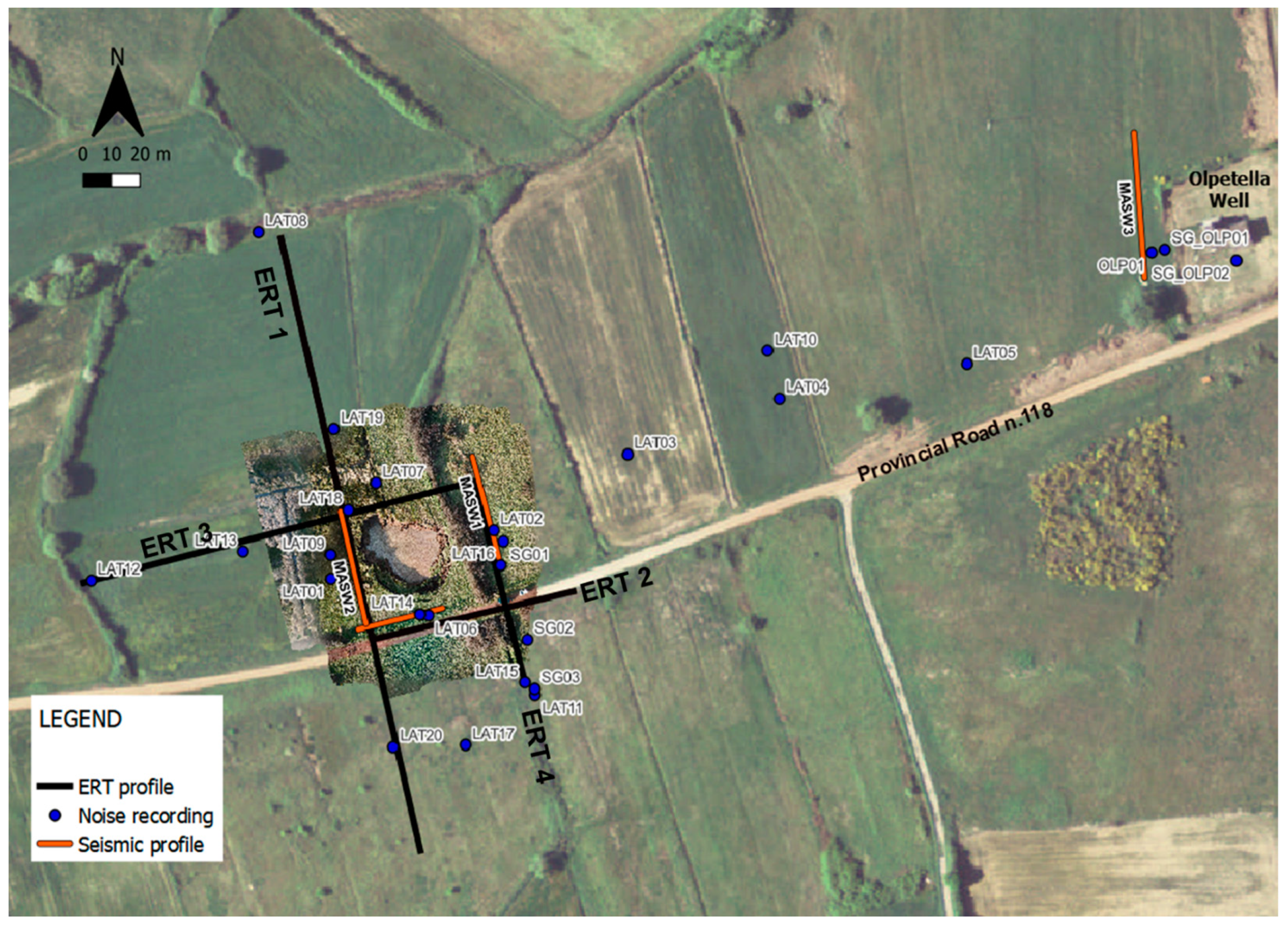
- Geophysical surveys to define a reliable subsurface model useful to address direct investigations (boreholes, geotechnical tests) and to image the collapsed area to possibly infer considerations on buried structures potentially responsible for the event.
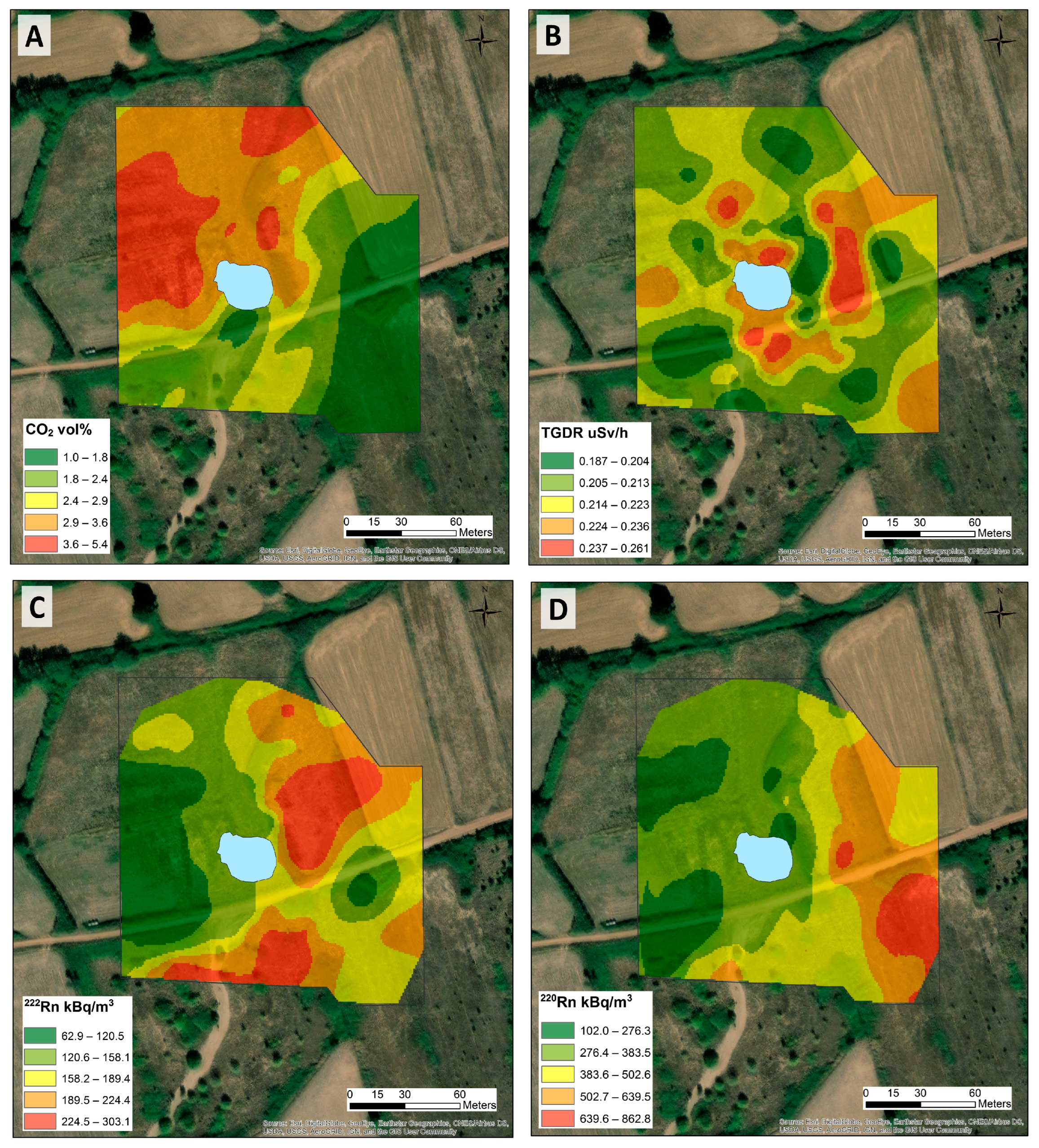
- Geochemical survey to highlight the presence of anomalous concentrations of soil gases, indicating the presence of advective gas migration from depth along major permeability pathways (e.g., faults and fractures) that may trigger the collapse.
2. Study Area
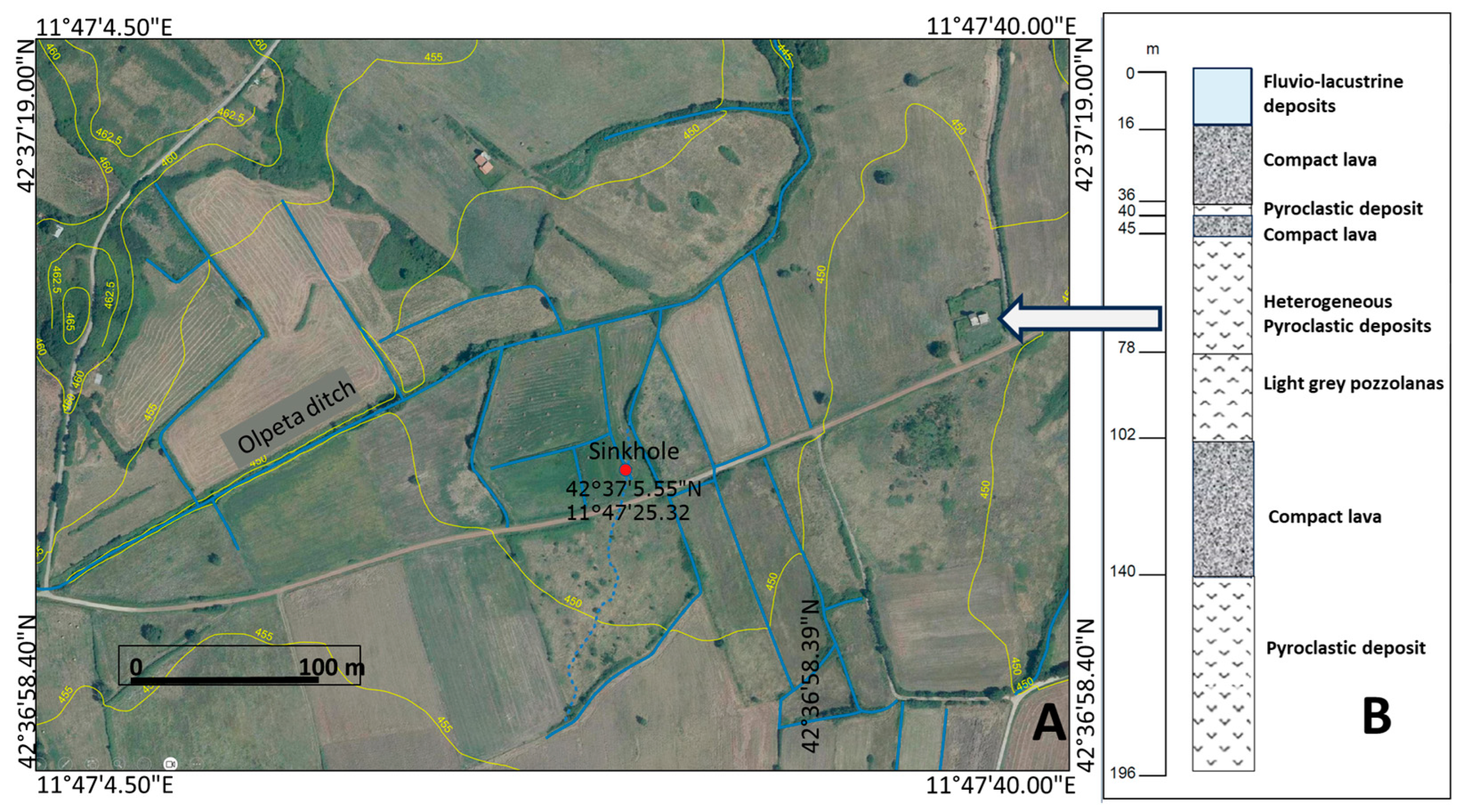
2.1. General Geological Setting
2.2. Stratigraphic Setting
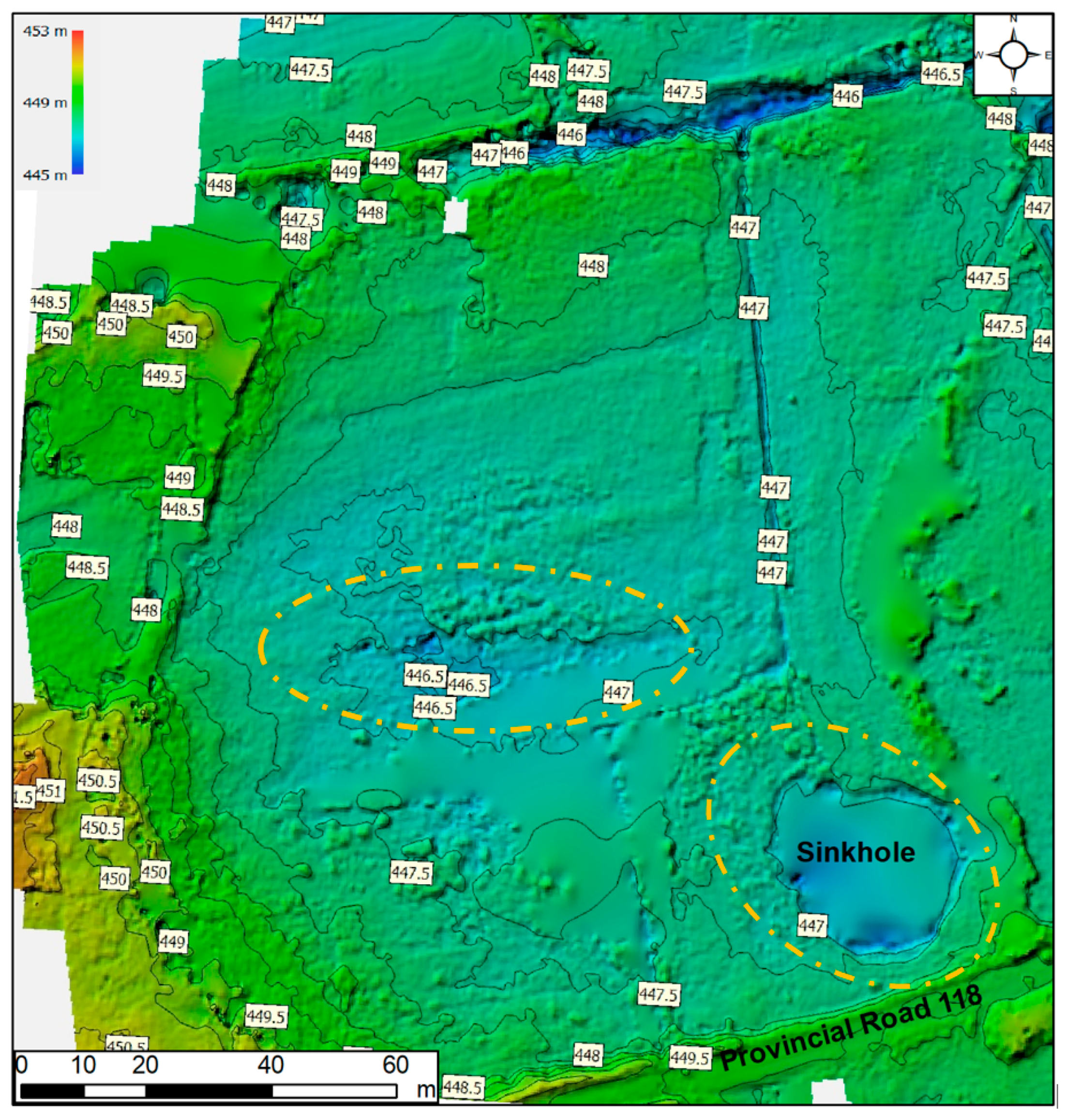
2.3. Morphological Setting
2.4. Climate
3. Materials and Methods
3.1. UAV Photogrammetric Surveys
- Image control and quality assessment to identify high-quality images to be used;
- Image alignment and preliminary sparse cloud elaboration;
- Attribution of a reference system (EPSG 3003) and positioning of marks in photographic images, with subdivision into ground control point (GCP) and control point (C.P.);
- Process of alignment optimization and gradual selection for error reduction;
- Heights map from high-quality, dense cloud generation;
- Elimination of low confidence points and classification of the dense cloud into terrain points;
- Generation of the final model using terrain points (DTM) and quality reduction from 1.5 cm/pixel to 20 cm/pixel;
- Generation of contour lines (50 cm interval);
- Creation of the textured 3D topographic model;
- Creation of the orthomosaic (1.15 cm/pixel).
3.2. Geophysical Methods
3.2.1. Electrical Resistivity Surveys
3.2.2. Surface-Wave Surveys
3.2.3. Ambient Vibration Recordings
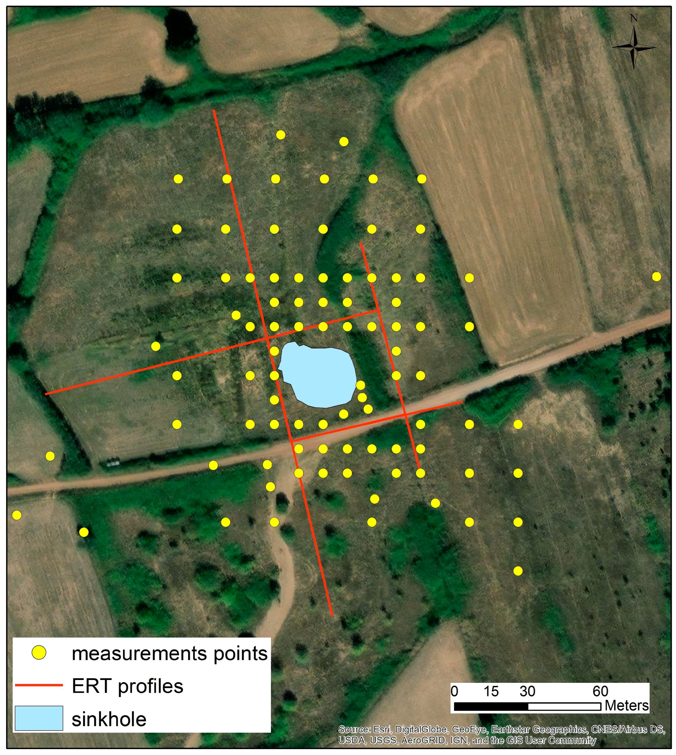
3.3. Geochemical Surveys
4. Results
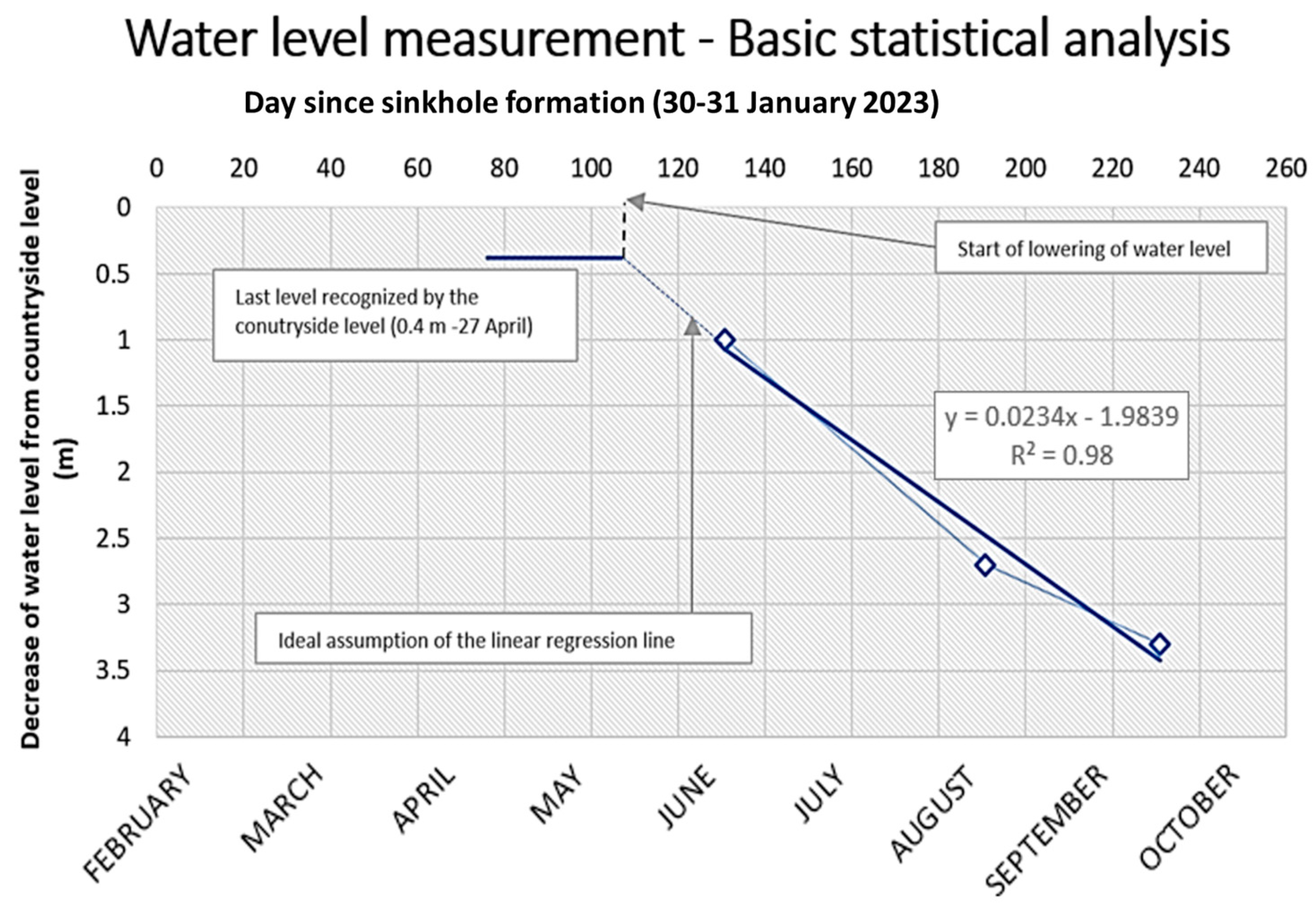
4.1. Photogrammetry
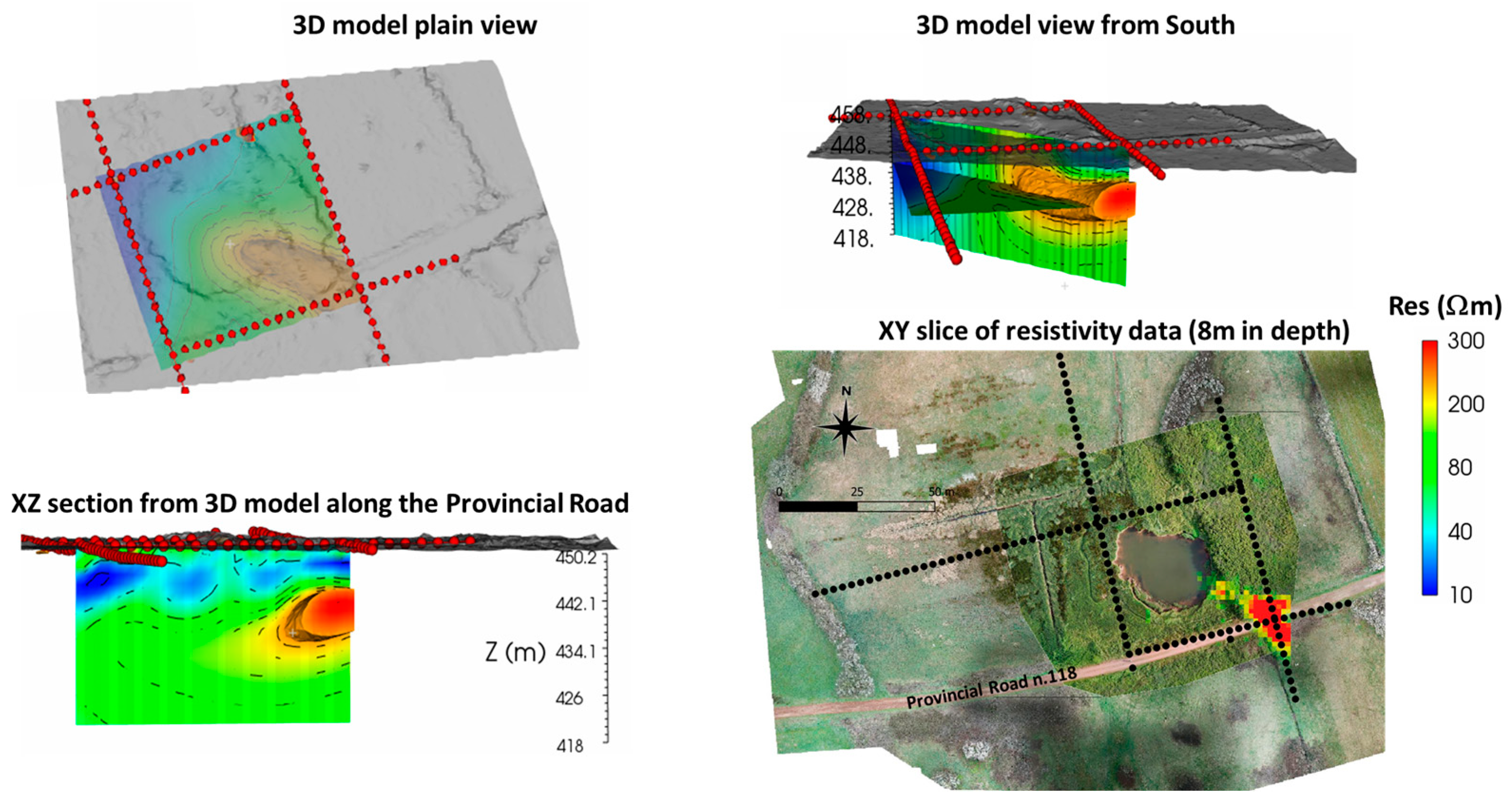
4.2. Resistivity Surveys
4.3. Surface-Wave Surveys
4.4. Ambient Vibration Recordings
4.5. Geochemical Survey
5. Discussion
6. Conclusions
Author Contributions
Funding
Data Availability Statement
Conflicts of Interest
References
- Fairbridge, R.W. The Encyclopedia of Geomorphology; Reinhold: New York, NY, USA, 1968; 1295p. [Google Scholar]
- Monroe, W.H. A Glossary of Karst Terminology; U.S. Geological Survey Water-Supply Paper; U.S. Government Publishing Office: Washinghton, DC, USA, 1970. [Google Scholar] [CrossRef]
- Beck, B.F. Sinkholes: Their Geology, Engineering & Environmental Impact; Balkema, A.A., Ed.; Rotterdam: Boston, MA, USA, 1984; 9p. [Google Scholar]
- Jennings, J.N. Karst Geomorphology; Basil Blackwell Ltd.: Oxford, UK, 1985; 293p. [Google Scholar]
- White, W.B. Geomorphology and Hydrology of Carbonate Terrains; Oxford University Press: Oxford, UK, 1988; 464p. [Google Scholar]
- Nisio, S. I fenomeni di sprofondamento: Stato delle conoscenze ed alcuni esempi in Italia Centrale. Alp. Mediterr. Quat. 2003, 16, 121–132. [Google Scholar]
- Caramanna, G.; Ciotoli, G.; Nisio, S. A review of natural sinkhole phenomena in Italian plain areas. Nat. Hazards 2008, 45, 145–172. [Google Scholar] [CrossRef]
- Calleja, I.; Tonelli, C. Dwejra and Maqluba: Emblematic Sinkholes in the Maltese Islands. In Landscapes and Landforms of the Maltese Islands; Gauci, R., Schembri, J., Eds.; Springer: Berlin/Heidelberg, Germany, 2019. [Google Scholar] [CrossRef]
- Waltham, A.C.; Fookes, P.G. Engineering Classification of Karst Ground Conditions. Q. J. Eng. Geol. Hydrogeol. 2005, 36, 101–118. [Google Scholar] [CrossRef]
- Waltham, T.; Bell, F.; Culshaw, M. Sinkholes and Subsidence; Springer: Berlin/Heidelberg, Germany; New York, NY, USA, 2003; 382p. [Google Scholar]
- De Waele, J.; Piccini, L.; Columbu, A.; Madonia, G.; Vattano, M.; Calligaris, C.; D’Angeli, I.M.; Forti, P. Evaporite karst in Italy: A review. Int. J. Speleol. 2017, 46, 137–168. [Google Scholar] [CrossRef]
- Galve, J.P.; Gutiérrez, F.; Lucha, P.; Bonachea, J.; Remondo, J.; Cendrero, A.; Gutiérrez, M.; Gimeno, M.J.; Pardo, G.; Sánchez, J.A. Sinkholes in the salt-bearing evaporite karst of the Ebro River valley upstream of Zaragoza city (NE Spain): Geomorphological mapping and analysis as a basis for risk management. Geomorphology 2009, 108, 145–158. [Google Scholar] [CrossRef]
- Gokkaya, E.; Gutierrez, F.; Ferk, M.; Gorum, T. Sinkhole development in the Sivas gypsum karst, Turkey. Geomorphology 2021, 386, 107746. [Google Scholar] [CrossRef]
- Parise, M.; Qiriazi, P.; Sala, S. Natural and anthropogenic hazards in karst areas of Albania. Nat. Hazards Earth Syst. Sci. 2004, 4, 569–581. [Google Scholar] [CrossRef]
- Tufano, R.; Guerriero, L.; Annibali Corona, M.; Bausilio, G.; Di Martire, D.; Nisio, S.; Calcaterra, D. Anthropogenic sinkholes of the city of Naples, Italy: An update. Nat. Hazards 2022, 112, 2577–2608. [Google Scholar] [CrossRef]
- Sinclair, W.C.; Stewart, J.W.; Knutilla, R.L.; Gilboy, A.E.; Miller, R.L. Types, Features, and Occurrence of Sinkholes in the Karst of West-Central Florida. Water-Resources Investigations Report. 1985. Available online: https://pubs.usgs.gov/wri/1985/4126/report.pdf (accessed on 10 November 2023).
- Nisio, S.; Caramanna, G.; Ciotoli, G. Sinkholes in Italy: First results on the inventory and analysis. Geol. Soc. Lond. Spec. Publ. 2007, 279, 23–45. [Google Scholar] [CrossRef]
- Gutiérrez, F.; Guerrero, J. A genetic classification of sinkholes illustrated from evaporite paleokarst exposures in Spain. Environ. Geol. 2008, 53, 993–1006. [Google Scholar] [CrossRef]
- Galve, J.P.; Casaneda, C.; Gutiérrez, F. Railway deformation detected by DInSAR over active sinkholes in the Ebro Valley evaporite karst, Spain. Nat. Hazards Earth Syst. Sci. 2015, 15, 2439–2448. [Google Scholar] [CrossRef]
- Baruffi, F.; Cisotto, A.; Cimolino, A.; Ferri, M.; Monego, M.; Norbiato, D.; Cappelletto, M.; Bisaglia, M.; Pretner, A.; Galli, A.; et al. Climate change impact assessment on Veneto and Friuli Plain groundwater. Part I: An integrated modeling approach for hazard scenario construction. Sci. Total Environ. 2012, 440, 154–166. [Google Scholar] [CrossRef] [PubMed]
- Barbieri, M.; Barberio, M.D.; Banzato, F.; Billi, A.; Boschetti, T.; Franchini, S.; Gori, F.; Petitta, M. Climate change and its effect on groundwater quality. Environ. Geochem. Health 2021, 45, 1133–1144. [Google Scholar] [CrossRef] [PubMed]
- Meng, Y.; Jia, L. Global warming causes sinkhole collapse—Case study in Florida, USA. Nat. Hazards Earth Syst. Sci. Discuss. 2018, 1–8. [Google Scholar] [CrossRef]
- Linares, R.; Roqué, C.; Gutiérrez, F.; Zarroca, M.; Carbonel, D.; Bach, J.; Fabregat, I. The impact of droughts and climate change on sinkhole occurrence. A case study from the evaporite karst of the Fluvia Valley, NE Spain. Sci. Total Environ. 2017, 579, 345–358. [Google Scholar] [CrossRef] [PubMed]
- Calligaris, C.; Forte, E.; Busetti, A.; Zini, L. A joint geophysical approach to tune an integrated sinkhole monitoring method in evaporitic environments. Near Surf. Geophys. 2023, 21, 317–332. [Google Scholar] [CrossRef]
- Argentieri, A.; Carluccio, R.; Cecchini, F.; Chiappini, M.; Ciotoli, G.; De Ritis, R.; Di Filippo, M.; Di Nezza, M.; Marchetti, M.; Margottini, S.; et al. Early stage sinkhole formation in the Acque Albule basin of central Italy from geophysical and geochemical observations. Eng. Geol. 2015, 191, 36–47. [Google Scholar] [CrossRef]
- Calligaris, C.; Zini, L.; Nisio, S.; Piano, C. Sinkholes in the Friuli Venezia Giulia Region: State of the art of the of territorial analyses in the evaporites. In Applied Geology: Approaches to Future Resource; Springer: Berlin/Heidelberg, Germany, 2020; Chapter 5; pp. 73–90. ISBN 978-3-030-43952-1. [Google Scholar] [CrossRef]
- Nof, R.N.; Baer, G.; Ziv, A.; Raz, E.; Atzori, S.; Salvi, S. Sinkhole precursors along the Dead Sea, Israel, revealed by SAR interferometry. Geology 2013, 41, 1019–1022. [Google Scholar] [CrossRef]
- Jones, C.E.; Blom, R.G. Bayou Corne, Louisiana, sinkhole: Precursory deformation measured by radar interferometry. Geology 2014, 42, 111–114. [Google Scholar] [CrossRef]
- Intrieri, E.; Gigli, G.; Nocentini, M.; Lombardi, L.; Mugnai, F.; Fidolini, F.; Casagli, N. Sinkhole monitoring and early warning: An experimental and successful GB-InSAR application. Geomorphology 2015, 241, 304–314. [Google Scholar] [CrossRef]
- Nappi, G.; Renzulli, A.; Santi, P. An evolutionary model for the Paleo-Bolsena and Bolsena volcanic complexes: A structural and petrographic study. Period. Mineral. 1987, 56, 241–267. [Google Scholar]
- Nappi, G.; Renzulli, A.; Santi, P. Evidence of incremental growth in the Vulsinian calderas (central Italy). J. Volcanol. Geotherm. Res. 1991, 47, 13–31. [Google Scholar] [CrossRef]
- Nappi, G.; Renzulli, A. Genesi ed evoluzione della caldera del Vepe (Complesso Vulcanico di Latera). Mem. Descr. Carta Geol. D’It. 1990, 38, 129–144. [Google Scholar]
- Turbeville, B.N. Tephra fountaining, rheomorphism, and spatter flow during emplacement of the Pitigliano Tuffs, Latera caldera, Italy. J. Volcanol. Geotherm. Res. 1992, 53, 309–327. [Google Scholar] [CrossRef]
- Vezzoli, L.; Conticelli, S.; Innocenti, F.; Landi, P.; Manetti, P.; Palladino, D.M.; Trigila, R. Stratigraphy of the Latera volcanic complex: Proposals for a new nomenclature. Period. Mineral. 1987, 56, 89–110. [Google Scholar]
- Capaccioni, B.; Nappi, G.; Renzulli, A.; Santi, P. The eruptive history of Vepe Caldera (Latera volcano) a model inferred from structural and geochemical data. Period. Mineral. 1987, 56, 269–283. [Google Scholar]
- Palladino, D.M.; Simei, S.; Trigila, R.; Acocella, V.; Baldini, A.; Bigi, S.; Fabbri, M.; Paccara, P.; Papacchini, P.; Petitta, M.; et al. Note Illustrative Della Carta Geologica d’Italia Alla Scala 1:50.000, Foglio n. 344 Tuscania. Palladino, D.M., Simei, S., Trigila, R., Eds.; 2020. Available online: https://www.isprambiente.gov.it/Media/carg/note_illustrative/344_Tuscania.pdf (accessed on 10 November 2023).
- Capelli, G.; Mastrorillo, L.; Mazza, R.; Petitta, M.; Baldoni, T.; Banzato, F.; Cascone, D.; Salvo, C.D.; Vigna, F.L.; Taviani, S.; et al. Hydrogeological Map of Latium Region 1:100.000 Scale (4 Sheets); S.E.L.CA: Firenze, Italy, 2012. [Google Scholar]
- Giraudi, C. Le oscillazioni di livello del lago di Mezzano (Valentano-VT): Variazioni climatiche e interventi antropici. Alp. Mediterr. Quat. 2004, 17, 221–230. [Google Scholar]
- Beck, H.E.; Zimmermann, N.E.; McVicar, T.R.; Vergopolan, N.; Berg, A.; Wood, E.F. Present and future Köppen-Geiger climate classification maps at 1-km resolution. Sci. Data 2018, 5, 180214. [Google Scholar] [CrossRef]
- Nakamura, Y. A Method for Dynamic Characteristics Estimation of Subsurface Using Microtremor on the Ground Surface; Railway Technical Research Institute, Quarterly Reports; Japan Railway Technical Research Institute/Tetsudo Gijutsu Kenkyujo: Tokyo, Japan, 1989; Volume 30, No. 1. [Google Scholar]
- Hasan, M.; Shang, Y.; Meng, H.; Shao, P.; Yi, X. Application of electrical resistivity tomography (ERT) for rock mass quality evaluation. Sci. Rep. 2021, 11, 23683. [Google Scholar] [CrossRef]
- Dahlin, T.; Zhou, B. A numerical comparison of 2D resistivity imaging with 10 electrode arrays. Geophys. Prospect. 2004, 52, 379–398. [Google Scholar] [CrossRef]
- Loke, M.H. Tutorial: 2-D and 3-D Electrical Imaging Surveys. 2023. Available online: http://www.geotomosoft.com/downloads.php (accessed on 10 November 2023).
- Loke, M.H.; Barker, R.D. Rapid least-squares inversion of apparent resistivity pseudosections using a quasi-Newton method. Geophys. Prospect. 1996, 44, 131–152. [Google Scholar] [CrossRef]
- Loke, M.H. Topographic modelling in resistivity imaging inversion. In Proceedings of the 62nd EAGE Conference & Technical Exhibition Extended Abstracts, Glasgow, UK, 29 May–2 June 2000. D-2. [Google Scholar]
- Morelli, G.; LaBrecque, D.J. Robust scheme for ERT inverse modeling. Eur. J. Environ. Eng. Geophys. 1996, 2, 1–14. [Google Scholar]
- Santarato, G.; Ranieri, G.; Occhi, M.; Morelli, G.; Fischanger, F.; Gualerzi, D. Three-dimensional electrical resistivity tomography to control the injection of expanding resins for the treatment and stabilization of foundation soils. Eng. Geol. 2011, 119, 18–30. [Google Scholar] [CrossRef]
- Telford, W.; Geldart, L.; Sheriff, R. Applied Geophysics, 2nd ed.; Cambridge University Press: Cambridge, UK, 1990. [Google Scholar] [CrossRef]
- Rahnema, H.; Mirassi, S.; Dal Moro, G. Cavity effect on Rayleigh wave dispersion and P-wave refraction. Earthq. Eng. Eng. Vib. 2021, 20, 79–88. [Google Scholar] [CrossRef]
- Glangeaud, F.; Mari, J.; Lacoume, J.-L.; Mars, J.; Nardin, M. Dispersive Seismic Waves in Geophysics. Eur. J. Environ. Eng. Geophys. 1999, 3, 265–306. [Google Scholar]
- Park, C.B.; Miller, R.D.; Xia, J. Multichannel analysis of surface waves. Geophysics 1999, 64, 800–808. [Google Scholar] [CrossRef]
- Xia, J.; Miller, R.D.; Park, C.B. Estimation of near-surface shear-wave velocity by inversion of Rayleigh waves. Geophysics 1999, 64, 691–700. [Google Scholar] [CrossRef]
- Foti, S.; Hollender, F.; Garofalo, F.; Albarello, D.; Asten, M.; Bard, P.Y.; Comina, C.; Cornou, C.; Cox, B.; Di Giulio, G.; et al. Guidelines for the good practice of surface wave analysis: A product of the InterPACIFIC project. Bull. Earthq. Eng. 2018, 16, 2367–2420. [Google Scholar] [CrossRef]
- Louie, J.N. Faster, Better: Shear-Wave Velocity to 100 Meters Depth from Refraction Microtremor Arrays. Bull. Seism. Soc. Am. 2001, 91, 347–364. [Google Scholar] [CrossRef]
- Asten, M. On bias and noise in passive seismic data from finite circular array data processed using SPAC methods. Geophysics 2006, 71, V153–V162. [Google Scholar] [CrossRef]
- Dal Moro, G. Surface Wave Analysis for Near Surface Applications; Elsevier: Amsterdam, The Netherlands, 2014; ISBN 9780128007709. [Google Scholar]
- Dal Moro, G.; Pipan, M. Joint inversion of surface wave dispersion curves and reflection travel times via multi-objective evolutionary algorithms. J. Appl. Geophys. 2007, 61, 56–81. [Google Scholar] [CrossRef]
- Dal Moro, G. Insights on surface wave dispersion and HVSR: Joint analysis via Pareto optimality. J. Appl. Geophys. 2010, 72, 129–140. [Google Scholar] [CrossRef]
- Ohori, M.; Nobata, A.; Wakamatsu, K. A comparison of ESAC and FK methods of estimating phase velocity using arbitrarily shaped microtremor analysis. Bull. Seism. Soc. Am. 2002, 92, 2323–2332. [Google Scholar] [CrossRef]
- Lin, S.; Ashlock, J. Surface-wave testing of soil sites using multichannel simulation with one receiver. Soil Dyn. Earthq. Eng. 2016, 87, 82–92. [Google Scholar] [CrossRef]
- Ibs-von Seht, M.; Wohlenberg, J. Microtremor measurements used to map thickness of soft sediments. Bull. Seism. Soc. Am. 1999, 89, 250–259. [Google Scholar] [CrossRef]
- SESAME Project (Site EffectS Assessment Using AMbient Excitations)-European Commission. General Directorate Project No. EVG1-CT-2000-00026. Guidelines for the Implementation of the H/V Spectral Ratio Technique on Ambient Vibrations: Measurements, Processing, and Interpretation. Deliverable 23.12. 2004. Available online: http://sesame.geopsy.org/Delivrables/Del-D23-HV_User_Guidelines.pdf (accessed on 10 November 2023).
- Bonnefoy-Claudet, S.; Cotton, F.; Bard, P.-Y. The nature of noise wavefield and its applications for site effects studies. A literature review. Earth-Sci. Rev. 2006, 79, 205–227. [Google Scholar] [CrossRef]
- Lunedei, E.; Albarello, D. Theoretical HVSR curves from full wavefield modelling of ambient vibrations in a weakly dissipative layered Earth. Geophys. J. Int. 2010, 181, 1093–1108. [Google Scholar] [CrossRef]
- Benà, E.; Ciotoli, G.; Ruggiero, L.; Coletti, C.; Bossew, P.; Massironi, M.; Mazzoli, C.; Mair, V.; Morelli, C.; Galgaro, A.; et al. Evaluation of tectonically enhanced radon in fault zones by quantification of the radon activity index. Sci. Rep. 2022, 12, 21586. [Google Scholar] [CrossRef]
- Sciarra, A.; Mazzini, A.; Inguaggiato, S.; Vita, F.; Lupi, M.; Hadi, S. Radon and carbon gas anomalies along the Watukosek Fault System and Lusi mud eruption, Indonesia. Mar. Pet. Geol. 2018, 90, 77–90. [Google Scholar] [CrossRef]
- Ciotoli, G.; Sciarra, A.; Ruggiero, L.; Annunziatellis, A.; Bigi, S. Soil gas geochemical behaviour across buried and exposed faults during the 24 August 2016 central Italy earthquake. Ann. Geophys. 2016, 59. [Google Scholar] [CrossRef]
- Etiope, G.; Martinelli, G. Migration of carrier and trace gases in the geosphere: An overview. Phys. Earth Planet. Int. 2002, 129, 185–204. [Google Scholar]
- Coletti, C.; Ciotoli, G.; Benà, E.; Brattich, E.; Cinelli, G.; Galgaro, A.; Massironi, M.; Mazzoli, C.; Mastacci, D.; Morozzi, P.; et al. The assessment of local geological factors for the construction of a Geogenic Radon Potential map using regression kriging. A case study from the Euganean Hills volcanic district (Italy). Sci. Total Environ. 2022, 808, 152064. [Google Scholar] [CrossRef] [PubMed]
- Giustini, F.; Ciotoli, G.; Rinaldini, A.; Ruggiero, L.; Voltaggio, M. Mapping the geogenic radon potential and radon risk by using Empirical Bayesian Kriging regression: A case study from a volcanic area of central Italy. Sci. Total Environ. 2019, 661, 449–464. [Google Scholar] [CrossRef] [PubMed]
- Giustini, F.; Ruggiero, L.; Sciarra, A.; Beaubien, S.E.; Graziani, S.; Galli, G.; Pizzino, L.; Tartarello, M.C.; Lucchetti, C.; Sirianni, P.; et al. Radon hazard in central Italy: Comparison among areas with different geogenic radon potential. Int. J. Environ. Res. Public Health 2022, 19, 666. [Google Scholar] [CrossRef]
- Annunziatellis, A.; Beaubien, S.E.; Bigi, S.; Ciotoli, G.; Coltella, M.; Lombardi, S. Gas migration along fault systems and through the vadose zone in the Latera caldera (central Italy): Implications for CO2 geological storage. Int. J. Greenh. Gas Control 2008, 2, 353–372. [Google Scholar] [CrossRef]
- Chiodini, G.; Baldini, A.; Barberi, F.; Carapezza, M.L.; Cardellini, C.; Frondini, F.; Granieri, D.; Ranaldi, M. Carbon dioxide degassing at Latera caldera (Italy): Evidence of geothermal reservoir and evaluation of its potential energy. J. Geophys. Res. Solid Earth 2007, 112. [Google Scholar] [CrossRef]
- Penman, H.L. Natural evaporation from open water, bare soil and grass. Proc. R. Soc. Lond. 1948, 193, 120–145. [Google Scholar] [CrossRef]
- Monteith, J.L. Evaporation and environment. Symp. Soc. Exp. Biol. 1965, 19, 205–234. [Google Scholar]
- Mori, F.; Mendicelli, A.; Moscatelli, M.; Romagnoli, G.; Peronace, E.; Naso, G. A new Vs30 map for Italy based on the seismic microzonation dataset. Eng. Geol. 2020, 275, 105745. [Google Scholar] [CrossRef]
- Pazzi, V.; Di Filippo, M.; Di Nezza, M.; Carlà, T.; Bardi, F.; Marini, F.; Fontanelli, K.; Intrieri, E.; Fanti, R. Integrated geophysical survey in a sinkhole-prone area: Microgravity, electrical resistivity tomographies, and seismic noise measurements to delimit its extension. Eng. Geol. 2018, 243, 282–293. [Google Scholar] [CrossRef]
- Pazzi, V.; Ceccatelli, M.; Gracchi, T.; Benedetta Masi, E.; Fanti, R. Assessing subsoil void hazards along a road system using H/V measurements, ERTs and IPTs to support local decision makers. Near Surf. Geophys. 2018, 16, 282–297. [Google Scholar] [CrossRef]
- Imposa, S.; Grassi, S.; Fazio, F.; Rannisi, G.; Cino, P. Geophysical surveys to study a landslide body (north-eastern Sicily). Nat. Hazards 2017, 86, 327–343. [Google Scholar] [CrossRef]
- Beaubien, S.E.; Ruggiero, L.; Annunziatellis, A.; Bigi, S.; Ciotoli, G.; Deiana, P.; Graziani, S.; Lombardi, S.; Tartarello, M.C. The importance of baseline surveys of near-surface gas geochemistry for CCS monitoring, as shown from onshore case studies in northern and southern Europe. Oil Gas Sci. Technol.–Rev. L’Inst. Fr. Pet. 2015, 70, 615–633. [Google Scholar] [CrossRef]
- Masruoğlu, G.; Altun, C.; Şentürk, M.Z.; Içhedef, M.; Taşköprü, C. Variation of soil gas 222Rn/220Rn concentration ratios along the Pınarbaşı segment of İzmir fault. J. Radioanal Nucl. Chem. 2023, 332, 4739–4743. [Google Scholar] [CrossRef]
- Baykara, O.; İnceöz, M.; Külahcı, F.; Doğru, M.; Aksoy, E. Assessment of 222Rn concentration and terrestrial gamma-radiation dose rates in the seismically active area. J. Radioanal Nucl. Chem. 2008, 278, 59–63. [Google Scholar] [CrossRef]
- Cinelli, G.; Tositti, L.; Capaccioni, B.; Brattich, E.; Mostacci, D. Soil gas radon assessment and development of a radon risk map in Bolsena, Central Italy. Environ. Geochem. Health 2015, 37, 305–319. [Google Scholar] [CrossRef]


| Site | Source | Impact | Geoph. | SW Comp. | Recording Time (s) | Samp. Rate (ms) |
|---|---|---|---|---|---|---|
| MASW1 | Active | V | H, V | ZVF, RVF | 2 | 0.125 |
| MASW2 | Active | V, H | H, V | ZVF, THF | 2 | 0.125 |
| MASW3 | Active | V | V | ZVF | 2 | 0.125 |
| ESAC/MASW | Active | V | V | ZVF | 2 | 0.125 |
| ESAC/MASW | Passive | V | V | Z | 420 | 8 |
| Survey Date (Month/Day/Year) | Water Level [m] |
|---|---|
| 02/01/2023 | 3.0 |
| 02/25/2023 | 0.4 |
| 03/30/2023 | 0.4 |
| 04/27/2023 | 0.4 |
| 06/09/2023 | 1.0 |
| 08/09/2023 | 2.7 |
| 09/18/2023 | 3.3 |
| Month | Rainfall | PET | Volume Loss (m3) |
|---|---|---|---|
| February | 28.8 | 38.3 | 26.81 |
| March | 67.4 | 61.6 | 43.12 |
| April | 59.4 | 89.3 | 62.51 |
| May | 87.2 | 107.3 | 75.11 |
| June | 75.6 | 138.9 | 97.23 |
| July | 10.2 | 37.2 | 26.04 |
| August | 43.3 | 157.9 | 110.53 |
| September 1 | 12.6 | 88.5 | 61.95 |
| Parameter | N | Mean | Median | Min | Max | Std. Dev. |
|---|---|---|---|---|---|---|
| CO2 vol% | 89 | 2.8 | 2.8 | 1.0 | 5.4 | 1.0 |
| O2 vol% | 89 | 19.6 | 19.7 | 18.3 | 20.9 | 0.6 |
| TGDR μSv/h | 89 | 0.218 | 0.217 | 0.187 | 0.261 | 0.014 |
| 222Rn kBq/m3 | 89 | 173.2 | 161.7 | 62.9 | 303.1 | 54.2 |
| 220Rn kBq/m3 | 89 | 399.4 | 349.5 | 102.0 | 862.8 | 142.4 |
Disclaimer/Publisher’s Note: The statements, opinions and data contained in all publications are solely those of the individual author(s) and contributor(s) and not of MDPI and/or the editor(s). MDPI and/or the editor(s) disclaim responsibility for any injury to people or property resulting from any ideas, methods, instructions or products referred to in the content. |
© 2024 by the authors. Licensee MDPI, Basel, Switzerland. This article is an open access article distributed under the terms and conditions of the Creative Commons Attribution (CC BY) license (https://creativecommons.org/licenses/by/4.0/).
Share and Cite
Puzzilli, L.M.; Ruscito, V.; Madonna, S.; Gentili, F.; Ruggiero, L.; Ciotoli, G.; Nisio, S. Natural Sinkhole Monitoring and Characterization: The Case of Latera Sinkhole (Latium, Central Italy). Geosciences 2024, 14, 18. https://doi.org/10.3390/geosciences14010018
Puzzilli LM, Ruscito V, Madonna S, Gentili F, Ruggiero L, Ciotoli G, Nisio S. Natural Sinkhole Monitoring and Characterization: The Case of Latera Sinkhole (Latium, Central Italy). Geosciences. 2024; 14(1):18. https://doi.org/10.3390/geosciences14010018
Chicago/Turabian StylePuzzilli, Luca Maria, Valerio Ruscito, Sergio Madonna, Francesco Gentili, Livio Ruggiero, Giancarlo Ciotoli, and Stefania Nisio. 2024. "Natural Sinkhole Monitoring and Characterization: The Case of Latera Sinkhole (Latium, Central Italy)" Geosciences 14, no. 1: 18. https://doi.org/10.3390/geosciences14010018