Physically Based and Empirical Ground Motion Prediction Equations for Multiple Intensity Measures (PGA, PGV, I_a, FIV3, CII, and Maximum Fourier Acceleration Spectra) on Sakhalin Island

Abstract

In the present study, empirical attenuation relations for multiple ground motion intensity measures (PGA, PGV, I_a, FIV3, CII, and MFAS) were developed for Sakhalin Island (in the far east of Russia). A recorded strong motion dataset was used, making GMPEs applicable in active crustal regions with an earthquake magnitude range of 4–6 and a distance range of up to 150 km. The hypocentral distance was used as a basic distance metric. For the first time in the research, an analytical representation of Arias intensity (I_a) was obtained in the framework of a multi-asperity source model. Asperities are considered as sub-sources of high-frequency incoherent radiation. The physical representation of the attenuation model in our study was based on a stress drop on the asperities and the ratio of the total rupture area to the combined area of asperities. The average stress drop on asperities for the examined earthquakes was approximately 13.4 MPa, and the ratio of the total rupture area to the asperity area was 0.22, which is generally close to similar estimates for crustal earthquakes. The coefficients and statistical scattering of the attenuation models were also analyzed. Moreover, a magnitude scale based on a modified Arias intensity is proposed in the present study. The new magnitude scale has an explicit physical meaning and is characterized by its simplicity of measurement. It is associated with the acceleration source spectrum level and can be successfully used in early warning systems.

1. Introduction

The investigation of physically based ground shaking measures and their use to conduct quantitative assessments of seismic hazard and risk factors is an urgent issue of earthquake engineering. The number of scientific articles devoted to the development of ground motion prediction equations increases every year (http://www.gmpe.org.uk, accessed on 1 June 2022); seismic intensity scales are also becoming more diverse in this area of research.

In addition to traditional ground shaking measures that can include simple peak measurements, such as PGA, PGV, or PGD, specialized metrics are also being used, which account for the amplitude and duration of a seismic signal. For example, the authors of [1] developed an attenuation model based on the maximum incremental ground velocity (MIV). The MIV is calculated for each horizontal component by integrating the acceleration record between two consecutive zero crossings. Essentially, this transformation provides an estimate of the area under the seismic pulse, and, therefore, accounts for the amplitude and duration of an individual pulse. The maximization of the new time series consisting of successive values of the areas (integrals) of each pulse presents the desired value of the maximum incremental velocity.

Cumulative absolute ground velocity (CAV) has been proposed in the literature as an instrumental indicator of structural damage (e.g., [2,3,4,5]). The CAV value is determined by the integration of the absolute acceleration over the whole seismic record. In [6], strong ground motion attenuation models were developed to obtain the CAV, its modification CAV₅ (when acceleration is above the 5 cm/s² threshold), and the standardized absolute velocity (CAVSTD). These models are applicable to shallow crustal and subduction (intra- and interplate) earthquakes with magnitudes ranging from 4 to 9 and distances of up to 400 km.

Another example of the practical consideration of incremental velocity is mentioned in [7]. Effective incremental ground velocity (EIGV) employed as a new ground shaking measure was proposed in this article. It was developed to predict the response of a rigid sliding block subjected to oscillations from a half-sinusoidal pulse. EIGV is a function of pulse duration, peak amplitude, and the coefficient of friction occurring between the basement and the sliding block.

The filtered incremental ground velocity (FIV3) is a recently proposed ground shaking measure [8]. An undeniable advantage of FIV3 over single-peak metrics is the measurement of several unipolar peak amplitudes, which should generally contribute to a more accurate prediction of the damage state of a risk element. In [9], the coefficients of the ground motion prediction equations used to perform multiple intensity measurements were analyzed, and it was concluded in the research that the FIV3 attenuation models were characterized by a relatively smaller standard deviation value compared to similar characteristics based on the measurements of a single-peak value.

In addition to engineering-consisted ground shaking metrics, a category of instrumental measures with physical meaning exists in the literature. Arias intensity (I_a) can be used to refer to such measures. It is determined by the integral of the quadratic acceleration. The spectral representation of the source time function according to the ${\omega }^2$-Brune model provides an analytical expression for the Arias intensity as a functional dependence on the source-to-site distance, earthquake magnitude, material parameters, and stress parameter [10,11]. The I_a metric has been successfully applied in research to assess earthquake-induced landslide hazards (e.g., [12,13]).

Generally, the idea of using Fourier acceleration spectra in engineering seismology has been suggested in the literature for quite a long period of time (e.g., [14]). A new instrumental intensity scale expressed through the average value of the high-frequency acceleration spectra (frequency band: 0.4–13 Hz) has been proposed [15]. The same study showed that macroseismic intensity, according to the modified Mercalli (MM) scale, correlated well with the parameters of the high-frequency spectra, and practically did not depend on regional features.

The development and physical interpretation of Fourier spectral attenuation models is an important part of recent seismological research [16,17]. It should be noted that the empirical characteristics of high-frequency (incoherent) radiation allow us to determine the physical parameters of the source. From the recent studies conducted on earthquake sources and rupture processes, it is known in the literature that high-frequency incoherent radiation is related to slip heterogeneity. Asperities are recognized as regions located on the fault that have large slips relative to the average slip of the rupture area. The asperity areas, as well as the entire rupture areas, scale with the total seismic moment. The size and stress drop of asperity are significant parameters for predicting strong ground motion parameters. These parameters are used as the input data in the technique of the stochastic simulation of seismic records (e.g., [18]). Therefore, the use of Fourier acceleration spectra simultaneously as engineering and physical measures is a practical method.

In addition to a variety of ground shaking measures utilized in the field, there are also various characteristics of the distance between the source and the site. Hypocentral distance (Rhyp) is quite suitable for point-source models, while other measures, such as Rrup (the closest distance between the site and the three-dimensional rupture plane) and Rjb (the shortest distance from a site to the surface projection of the rupture plane), are most commonly used for finite sources. The role of high-frequency radiation is also reflected in modified distance metrics (e.g., [19]).

Therefore, different strong ground motion metrics are used in various applied scenarios. For example, PGA/PGV are most commonly used to perform seismic hazard assessments. Arias intensity (I_a) is most commonly used to conduct seismic risk assessments, including geotechnical and structural applications. The use of the FIV3 metric has recently been proposed in the literature. It is used consistently with the potential-damage-assessment method. Although this metric is not as popular as PGA, PGV, or I_a, in our study we use FIV3 for empirical-testing purposes and for the comparison of ground motion equations with the most commonly used strong ground motion metrics. Additionally, we examine high-frequency spectral measurements, such as high-frequency Arias intensity and maximum Fourier acceleration spectra.

In this paper, regional attenuation equations based on the measures of PGA, PGV, I_a, FIV3, CII, and maximum Fourier acceleration spectra (MFAS) are developed. A recorded strong motion dataset and felt reports are also used. The study area is considered an active crustal region. We analyzed the statistical scattering of ground motion prediction equations. A physical interpretation of the coefficients is presented within the framework of the multi-asperity source model. Attenuation equations for the multiple intensity measures are developed for the first time for the target area.

2. Materials and Methods

2.1. Materials

2.1.1. Study Area and Tectonic Settings

The study area is located on Sakhalin Island and the surrounding shelf (Russia). The island is located in the northwestern part of the Pacific Ring of Fire, which is a continent-to-ocean transition zone with a powerful system of meridional faults (Figure 1). The boundary of the Okhotsk (or North American) and Amur (or Eurasian) plates is identified by these faults. The plate convergence velocity is 10–13 mm/year [20].

The interaction of the Amur and Okhotsk plates generates crustal seismicity, both at the boundaries and the periphery (Figure 1). Strong earthquakes occur quite frequently at this location. The largest earthquake (Mw 7.3) occurred in 1971 in the south of the island, far from settlements. However, the 1995 Neftegorsk earthquake (Mw 7) was the most catastrophic event and killed more than 2000 people (in the north of the island).

The study area is located in the active crustal region with shallow seismicity (source depth up to 30 km), according to the classification proposed in [21]. The focal mechanisms are most commonly reverse or thrust faults, and, more rarely, strike-slip [22].

2.1.2. Strong Motion Database

The strong motion recordings were collected as a result of long-term seismic monitoring and routine earthquake data-processing techniques. The duration of the recordings did not exceed three minutes. All the recordings were instrumentally corrected to an accelerogram measured in nm/s².

Crustal earthquakes with source depths of up to 30 km were considered in the present study (Figure 2). The magnitude ranged from ML 4 to 6.1. We selected records with epicentral distances up to 150 km in order to parameterize the geometric spreading of body waves by a term close to $1/r$.

All recordings were preprocessed. The corresponding intensity measures were selected from each station component. All selected values were placed into the database (see Data Availability Statement). Figure 2 presents the distribution of the selected data on a magnitude–distance plot. The total numbers of recordings, earthquakes, and stations in the dataset were 285, 28, and 22, respectively.

Local and moment magnitudes were tested in the attenuation relations. The calibration equation used to calculate the local magnitude is presented in [23]. Moment magnitude values were imported from earthquake data centers: USGS (https://www.usgs.gov/, accessed on 1 June 2022) and GFZ (https://www.gfz-potsdam.de/en/home/, accessed on 1 June 2022). If the moment magnitude was unavailable in the earthquake list, the magnitude conversation to the Mw scale was applied using global intermagnitude relations [24]. This was achieved by the polynomial approximation of the cubic-type equation:

$$\mathrm{M}\mathrm{w}=0.05\times {\mathrm{M}\mathrm{L}}^3-0.64\times {\mathrm{M}\mathrm{L}}^2+3.50\times \mathrm{M}\mathrm{L}-2.89.$$

(1)

Almost all of the instrumental sites were classified as soil category D according to the NEHRP classification [25]. The average measured S-wave velocity in the upper 30 m ground layer (V_S30) was 300–400 m/s (see Data Availability Statement). In our study, we proposed using a site term from Japanese GMPEs that was characterized by the similar reference V_S30.

2.1.3. Felt Reports

In addition to the instrumental ground shaking measures utilized in the research, the community Internet intensity (CII) derived from felt reports was considered in the present study. For this purpose, questionnaires in Russian were used in accordance with the regionalized technique DYFI? [26,27]. Felt reports were collected through the webpage of the regional seismological service eqalert.ru or its mobile applications (see Data Availability Statement).

Between 1 August 2016 and 30 April 2022 771 questionnaires were completed, with over 600 responses reported by Sakhalin respondents. The magnitude versus distance distribution of the processed macroseismic intensity is presented in Figure 2. The figure indicates that large earthquakes with ML 5–6 magnitudes are felt at distances up to 200 km from the epicenter. The total amount of CII measures is 131. The number of CIIs with two or more felt reports is 83.

2.2. Methods

2.2.1. Intensity Measures

For the first time in the research, we considered the maximum Fourier acceleration spectra (MFAS) as an intensity measure. We also introduced a modified Arias intensity (see

Table 1. List of the ground shaking measures considered in the study.

Measure	Equation
$PGA$, peak ground acceleration (cm/s2)	$\underset{t\in T}{\max }\left|a\left(t\right)\right|$
$PGV$, peak ground velocity (cm/s)	$\underset{t\in T}{\max }\left|\underset{0}{\overset{t}{\int }}a\left(\tau \right)d\tau \right|$
$I_a$, Arias intensity (m/s)	${\displaystyle \sum _{i=NS,EW}}\frac{\pi }{2g}\underset{0}{\overset{T}{\int }}{\left[a_i\left(t\right)\right]}^{2}dt$
$I_a\left(1\right)$, modified Arias intensity (m/s)	${\displaystyle \sum _{i=NS,EW}}\frac{\pi }{2g}\underset{0}{\overset{T}{\int }}{\left[a_{HP1}^{\left(i\right)}\left(t\right)\right]}^{2}dt$
$I_a\left(3\right)$, modified Arias intensity (m/s)	${\displaystyle \sum _{i=NS,EW}}\frac{\pi }{2g}\underset{0}{\overset{T}{\int }}{\left[a_{HP3}^{\left(i\right)}\left(t\right)\right]}^{2}dt$
$FIV3\left(T_0\right)$, filtered incremental velocity (cm/s)	$FIV3\left(T_0\right)=\max \left\{V_{max1}+V_{max2}+V_{max3},\left|V_{min1}+V_{min2}+V_{min3}\right|\right\}$, where $V\left(t\right)={\int }_t^{t+\alpha T_0}{a}_{LP1}\left(\tau \right)d\tau$
$MFAS$, maximum Fourier acceleration spectra (m/s)	$\mathit{MFAS}=\underset{f\in \mathsf{\Omega }}{\max }{\left(\begin{array}{c}{\left|\underset{0}{\overset{T}{\int }}{a}_{NS}\left(t\right)e^{2\pi ift}dt\right|}^2+\\ {\left|\underset{0}{\overset{T}{\int }}{a}_{EW}\left(t\right)e^{2\pi ift}dt\right|}^2\end{array}\right)}^{0.5}$

). The physical meaning of these metrics is discussed below.

We calculated the Fourier amplitude spectrum of the horizontal-component acceleration combined with the quadratic mean value. Such spectral representations are closely related to the amplitudes of SH-wave. The maximum value of the amplitude spectrum was referred to as the MFAS metric. Arias intensity was defined as the sum of all the squared acceleration values obtained from the horizontal records. For further details, see Table 1.

For the other measurements, the maximum values of the two horizontal (NS and EW) station components were selected. The filtered incremental ground velocity (FIV3) was computed for several natural oscillation periods: 0.01, 0.2, 1, and 3 s.

Table 1 summarizes the intensity measures, for which regional attenuation relationships were developed, and the corresponding transformations over signals of the original accelerogram $a\left(t\right)$, where:

$T$ is the duration of record;

$T_0$ is the natural period of oscillation;

$\alpha$ is the parameter (0.7, according to ([9]);

$\mathsf{\Omega }$ is the spectral domain;

$g$ is the acceleration of gravity (9.81 m/s²);

LP1 is the notation of a second-order low-pass Butterworth filter with a cut-off frequency of 1 Hz;

HP1 is the notation of a second-order high-pass Butterworth filter with a cut-off frequency $f_H$ = 1 Hz;

HP3 is the notation of a second-order high-pass Butterworth filter with a cut-off frequency $f_H$ = 3 Hz;

NS and EW are the north–south and east–west directions of the horizontal recordings, respectively.

As an example of ground shaking intensity measurements, we considered a moderate earthquake with an ML 4.5 magnitude and a source depth of 8.6 km, which occurred on 18 April 2021 on Sakhalin Island. Several buildings closest to the epicenter settlement (Rhyp = 9.5 km) were lightly damaged. The macroseismic Internet intensity level derived from the felt reports was approximately CII = 6.3. The accelerograph located in this settlement recorded strong ground motions. The original records and transformations over signals are presented in Figure 3. The corresponding quadratic acceleration spectrum is shown in Figure 4.

The felt reports in each locality were reduced to the community weighted sum (CWS), taking into account various indicators of ground motion activity in accordance with [26]:

$$\mathrm{C}\mathrm{W}\mathrm{S}=5\times \mathrm{F}\mathrm{e}\mathrm{l}\mathrm{t}+\mathrm{M}\mathrm{o}+\mathrm{R}\mathrm{e}+2\times \mathrm{S}\mathrm{t}+5\times \mathrm{S}\mathrm{h}+2\times \mathrm{P}\mathrm{i}\mathrm{c}+3\times \mathrm{F}\mathrm{u}\mathrm{r}+5\times \mathrm{D}\mathrm{a}\mathrm{m},$$

(2)

where Felt is the “felt” index (values from 0 to 1); Mo is the “motion” index (values from 0 to 5); Re is the “reaction” index (values from 0 to 5); St is the “stand” index (values from 0 to 1); Sh is the “shelf” index (values from 0 to 3); Pic is the “picture” index (values from 0 to 1); Fur is the “furniture” index (values from 0 to 1); and Dam is the “damage” index (values from 0 to 3).

Then, the decimal value of the community Internet intensity (CII) is calculated and rounded to the first decimal place (if CWS ≥ 6.53):

$$\mathrm{C}\mathrm{I}\mathrm{I}=3.4\times \ln \mathrm{C}\mathrm{W}\mathrm{S}-4.38.$$

(3)

If CWS < 6.53, but the earthquake was felt (Felt > 0), then CII = 2 is obtained; if it was not felt (Felt = 0), then CII = 1.

2.2.2. Attenuation Model

The study area was comparable to a neighboring seismically active region (Japan) in terms of the tectonics and soil conditions. The reference value of the S-wave velocity in a 30 m soil layer was 350 m/s [28,29]. This was closely related to the soil conditions in Sakhalin Island.

The point-source model is most commonly used in the field for seismic sources where Mw < 5.5. We considered earthquakes with magnitude values up to Mw 5.8. The nearest instrumental site for an Mw 5.8 earthquake is located at the hypocentral distance of 21.5 km. Therefore, we proposed that the finite-fault effects for distances greater than 21.5 km were negligible. The point-source approximation seemed to be reasonable for a given magnitude and the distance ranges. Therefore, the following attenuation model was considered:

$${IM}_{ij}=a\times {\mathrm{M}}_i-k\times \lg R_{ij}-b\times R_{ij}+c\pm \sigma \times {\epsilon }_{ij},$$

(4)

where ${IM}_{ij}$ is the intensity measure (macroseismic intensity or logarithm of instrumental measure) of the i-th earthquake at the j-th seismic station; $a$, $k$, $b$, and $c$ are the regression parameters to be estimated; $\sigma$ is the standard deviation of the empirical attenuation model; ${\mathrm{M}}_i$ is the magnitude of the i-th earthquake; $R_{ij}$ is the hypocentral distance from the i-th source to the j-th seismic station; and ${\epsilon }_{ij}$ is a $N\left(\mathrm{0,1}\right)$ normally distributed random variable with zero mean and unit variance.

For the last 25 years mixed-effects regressions have been the standard approach in the research used for GMPEs to account for correlations in the data. The alternative approach that is widely used in Japan is the two-step stratified regression analysis method (e.g., [30,31]). This method was proposed by Joyner and Boore [32] to avoid the interaction between the coefficients $a$ and $k$. In other words, errors produced when measuring earthquake magnitudes would affect the distance coefficient obtained from the ordinary least squares regression. In recent decades, the accuracy of moment magnitude determination has significantly increased. The ordinary least squares regression method seemed to be appropriate for this dataset. Therefore, the best coefficients of the model (4) were fitted by multiple linear regression. We analyzed the interaction between the magnitude and distance terms by fixing the coefficients $a$ and/or $k$ at their physical values (see Section 3.1). The standard deviation ($\sigma$) was considered as the basic metric of the statistical scatter. Additionally, the coefficient of determination ($R^2$) was used for each model representation. The statistical parameter $R^2$ is a metric of the quality of fit between the predicted and observed data, and it is expressed in relative units.

2.2.3. Physical Representation of High-Frequency Measures

The idea of developing physically based GMPEs was proposed in [33]. Hanks and McGuire used Parseval’s theorem, which states that the integral of the square of a function is equal to the integral of the square of its Fourier transform.

In [10], a source-related acceleration spectrum was modeled by the simplified band-limited function. It obtains constant values between a lower frequency, related to the source size, and an upper bounding frequency, related to the upper-crustal attenuation. The source spectrum was proposed to be zero outside the mentioned frequency range. Geometrical spreading was considered as a major attenuation factor. Anelastic attenuation was neglected. As a result, semi-empirical relations between the Arias intensity, moment magnitude, source-to-site distance, and static stress drop were derived.

In their study, Stafford et al. [11] considered a more general case where the earthquake acceleration spectrum was given by the multiplication of the attenuation and source functions. The authors proposed a ${\omega }^2$-Brune spectrum in the framework of a single-crack source model. The attenuation was described by geometrical spreading and the frequency-independent Q-factor.

In our study, we introduced an improved analytical predictive equation to obtain the Arias intensity. We collected all the attenuation functions, such as frequency-dependent anelastic attenuation, upper-crustal attenuation, the upper-crustal amplification factor, and geometrical spreading attenuation. The novelty of the presented approach was that high-frequency radiation was described in terms of the multi-asperity source model.

Considering the fragmented structure of the earthquake source, many researchers (e.g., [18,34,35] and others) concluded that there were spots located on the fault plane characterized by increased values of the strength. Such spots are referred to asperities. Asperities are relatively small and occupy 10–30% of the total rupture area. They are sub-sources of incoherent high-frequency radiation on small space–time scales. The average stress drop on asperities is 10 (sometimes more) times greater than the average stress drop over the fault, which is approximately 3 MPa.

Once the largest asperity has been determined, it is possible to estimate the stress drop of the same asperity ($∆\tau$) using the flat level of the acceleration spectra ($A_0$) given by the following equation [34]:

$$A_0\cong \frac{A_a}{0.98}\cong \frac{\sqrt{S_a}∆\tau }{\sqrt{\pi }\rho \beta },$$

(5)

where $\rho$ and $\beta$ are the density and shear-wave velocity in the vicinity of the source, respectively, and $S_a$ is the area of asperity.

Generally, the amplitude acceleration spectrum of the S-wave can be written as

$$A\left(f\right)=A_0\times As\left(f\right)\times G\left(R\right)\times Ae\left(f,R\right)\times Am\left(f\right)\times An\left(f\right),$$

(6)

where $f$ is the frequency, $As\left(f\right)$ is the source-related acceleration spectrum (the shape of the spectrum), $G\left(R\right)$ is the attenuation attributed to the geometrical spreading, $Ae\left(f,R\right)$ is the anelastic whole-path attenuation factor, $Am\left(f\right)$ is the upper-crustal amplification factor, and $An\left(f\right)$ is the upper-crustal attenuation factor.

Recent studies conducted on earthquake spectra corrected for the attenuation functions showed that their shape was complicated by several corner frequencies [36]. However, the approximation of the observed spectra by the ${\omega }^2$ model seems to be quite reasonable (e.g., [37,38]). Therefore, to simplify the theoretical calculations, the shape of the source-related acceleration spectrum is presented by the following equation:

$$As\left(f\right)=\frac{f^2}{f_{\mathrm{c}}^2+f^2},$$

(7)

where $f_c$ is the corner frequency associated with the source dimension.

For distances that do not exceed 150 km, the geometrical spreading function $G\left(R\right)$ can be written as

$$G\left(R\right)=\frac{1}{R_0}{\left(\frac{R_0}{R}\right)}^{\zeta },$$

(8)

where $R_0$ is a reference distance, usually set as being equal to 1 km, and $\zeta$ is the indicator of the geometrical spreading.

The anelastic whole-path attenuation factor is presented by the following equation:

$$\mathit{Ae}\left(f,R\right)=\exp \left(-\frac{\pi fR}{Q\left(f\right)\beta }\right),$$

(9)

where $Q\left(f\right)$ is the quality factor as a function of frequency $f$.

In order to determine the necessary attenuation characteristics, the study area was examined in the framework of the single back-scattering model [39]. The quality factor $Q\left(f\right)$ was determined by

$$Q\left(f\right)=Q_{0}f,$$

(10)

where $Q_0$ is the constant.

In general, a functional dependence in (10) was typical for active crustal regions. For example, a similar dependence was obtained in Japan for the crustal type of seismicity (e.g., [40]).

The amplification factor was calculated by solutions that accounted for the seismic energy conversation in the upper crust. According to [37], $Am\left(f\right)$ is determined by the square root of the impedance ratio between the source and surface, that is,

$$Am\left(f\right)=\sqrt{\frac{\rho \beta }{{\rho }_1{\beta }_1}},$$

(11)

where ${\rho }_1$ and ${\beta }_1$ are the time-weighted average values from the surface to a depth equivalent to a quarter wavelength density and shear-wave velocity, respectively.

The upper-crustal attenuation factor, which represents the attenuation of waves in the upper 4 km of the Earth’s crust, is defined by a generalization of Equation (9):

$$An\left(f\right)=\exp \left(-\pi \kappa f\right),$$

(12)

where $\kappa$ is the “kappa” parameter.

By substituting (10) into (9) and then (5), (7)–(9), and (12) into (6), we obtained an analytical representation of the amplitude spectrum of the accelerogram containing the S-wave:

$$A\left(f\right)=\frac{FV}{\sqrt{\pi }\rho \beta R_0}\times \sqrt{k_{f}S}\times ∆\tau \times {\left(\frac{R_0}{R}\right)}^{\zeta }\times \frac{f^2}{f_{\mathrm{c}}^2+f^2}\times \exp \left(-\frac{\pi fR}{Q\left(f\right)\beta }\right)\times Am\left(f\right)\times \exp \left(-\pi \kappa f\right),$$

(13)

where $F$ is the free surface factor (usually set as being equal to 2) and $V$ is the factor partitioning energy into two orthogonal directions (usually set as being equal to $1/\sqrt{2}$).

Equation (13) accounts for the filling factor $k_f$ given by the ratio of the total rupture area ($S$) to the combined area of asperities ($S_a$):

$$\frac{S_a}{S}=k_f.$$

(14)

According to Parseval’s theorem,

$${\int }_{-\infty }^{+\infty }{\left|a\left(t\right)\right|}^{2}dt={\int }_{-\infty }^{+\infty }{\left|A\left(f\right)\right|}^{2}df.$$

(15)

The seismic record is defined by the time interval $\left[0,T\right]$, where the signal at each moment in time is produced by a real value. Formally, we considered that, outside the specified time interval, the signal was zero. Then, accounting for the conditions,

$$a\left(t\right)=0\mathrm{if}\left\{\begin{array}{c}t<0,\\ t>T\end{array}\right.$$

(16)

and

$$A\left(f\right)=A\left(-f\right),$$

(17)

we can rewrite (15) as

$${\int }_{-\infty }^{+\infty }{\left|a\left(t\right)\right|}^{2}dt={\int }_0^T{\left|a\left(t\right)\right|}^{2}dt={\int }_{-\infty }^{+\infty }{\left|A\left(f\right)\right|}^{2}df=2{\int }_0^{+\infty }{\left|A\left(f\right)\right|}^{2}df.$$

(18)

Accounting for (18), the Arias intensity can be written as

$$I_a=\frac{\pi }{2g}{\int }_0^T{\left[a\left(t\right)\right]}^{2}dt=\frac{\pi }{g}{\int }_0^{+\infty }{\left|A\left(f\right)\right|}^{2}df.$$

(19)

Furthermore, by substituting (13) into (19), following the elementary transformations, we obtained the subsequent expression:

$$I_a=\frac{F^2{V}^2{k}_f{\overline{Am}}^2{∆\tau }^2}{g{\rho }^2{\beta }^2{R}_0^2}S\times {\left(\frac{R_0}{R}\right)}^{2\zeta }\times \exp \left(-\frac{2\pi fR}{Q_0\beta }\right)\times \frac{\mathsf{\Psi }}{2\pi \kappa },$$

(20)

where

$$\mathsf{\Psi }=\lambda {\int }_0^{+\infty }\frac{\exp \left(-\lambda x\right)x^4}{{\left[1+{\left(x\right)}^2\right]}^2}dx,$$

(21)

$$\lambda =2\pi \kappa f_c.$$

(22)

We considered the frequency-independent amplification factor denoted by $\overline{Am}$.

In their study, Stafford et al. [11] showed that the parameter $\mathsf{\Psi }$ was close to 1 and possible deviations from 1 did not exceed 20%. We numerically integrated the expression presented in (21) and entered the results in a graph depending on $\lambda$ (see Figure 5). At relatively small values of the variable $\lambda$, parameter $\mathsf{\Psi }$ was close to 1. For example, for $\kappa$ = 0.03 and $f_c$ = 1, parameter Ψ was equal to 0.698 ($\lambda$ = 0.188). Therefore, at $f_c$ < 1 (which corresponds to the considered magnitude range), this approximation seemed to be quite reasonable.

Empirical relationships between earthquake magnitude and source parameters were used in this study [18,35,41,42]:

$$\lg M_0=1.5\lg S+\lg ∆\sigma +\lg \frac{16}{7{\pi }^{3/2}},$$

(23)

$$\mathrm{M}\mathrm{w}=\frac{2}{3}\left(\lg M_0-9.1\right),$$

(24)

$$∆\sigma =k_f∆\tau ,$$

(25)

where $M_0$ is the seismic moment, $\mathrm{M}\mathrm{w}$ is the moment magnitude, and $∆\sigma$ is the stress drop of the circular source; the parameters $k_f$ and $∆\tau$ are most commonly referred to as inner fault parameters, while $M_0$ and $∆\sigma$ are referred to as the outer characteristics of the source.

By taking the logarithm of (20), accounting for (23)–(25), we obtained an analytical attenuation equation for the I_a metric:

$$\lg I_a=\mathrm{M}\mathrm{w}-2\zeta \lg R-\frac{2\pi \lg e}{Q_0\beta }R+c^{\prime },$$

(26)

where

$$c^{\prime }=\lg c_0+\frac{18.2}{3}+\lg \left(k_f^{1/3}{∆\tau }^{4/3}\right),$$

(27)

$$c_0={\left(\frac{7}{16}\right)}^{2/3}\frac{F^2{V}^2{\overline{Am}}^2}{2\kappa g{\rho }^2{\beta }^2{R}_0^2}.$$

(28)

By comparing (4) and (26), we concluded that the produced attenuation model was identical to the physical representation of the intensity I_a; the coefficients of Model (4) corresponded to the following physical constants obtained from (26): $a=1$, $k=2\zeta$, $b=\frac{2\pi \lg e}{Q_0\beta }$, and $c=c^{\prime }$. Once the empirical constants are determined, it is possible to estimate the stress drop of asperity:

$$∆\tau =\frac{{10}^{\frac{3c}{4}-4.55}}{c_0^{\frac{3}{4}}{k}_f^{1/4}}.$$

(29)

In [43], the empirical relation between V_S30 and $\kappa$ was developed using instrumental measures obtained from the dense seismic network KiK-net in Japan. For the range 155 < V_S30 < 2000 m/s, the “kappa” parameter monotonically decreases with the increasing V_S30 value. Therefore, the global (or regional) V_S30 maps in combination with the abovementioned empirical relation can be used to parameterize the “kappa” attenuation within the physical representation of the attenuation equation.

For the modified metrics I_a(1) and I_a(3), according to their definitions presented in Table 1, the magnitude–distance relations will be similar to (26); the constant $c_0$ in this case will be produced by the following expression:

$$c_0={\left(\frac{7}{16}\right)}^{2/3}\frac{F^2{V}^2{\overline{Am}}^2}{2\kappa g{\rho }^2{\beta }^2{R}_0^2}\exp \left(-2\pi \kappa f_H\right),$$

(30)

where $f_H$ = 1 Hz or $f_H$ = 3 Hz.

Expression (30) was obtained under the assumption ($f_H>f_c$), where the source acceleration spectrum (7) was presented by the flat level.

The spectral metric MFAS has a physical meaning similar to that of I_a. Gusev [35] considered a multi-asperity source model in his study, assuming that the ratio of the total rupture area to the combined area of asperities was constant. He obtained an analytical expression where the maximum value of the acceleration spectrum, corrected for the attenuation functions and geometrical spreading, was produced by the functional dependence on the source radius and the stress drop on asperities; that is,

$$MFAS~\sqrt{S}∆\tau .$$

(31)

Therefore, the high-frequency metrics I_a and MFAS were dependent on inner and outer fault parameters. These parameters were more closely related to the generation of strong motions occurring in the near-source zone. Once these parameters were determined in the target region, it allowed us to follow a method proposed by Irikura [18] in order to successfully obtain stochastically simulated ground motion parameters.

Table 2. Physical constants and material parameters used in the study.

Parameter	Value
$F$	2
$V$	1
$\overline{Am}$	2
$\kappa$	0.03 s
$\rho$	2700 kg/m3
$\beta$	3300 m/s
$R_0$	1000 m
$g$	9.81 m/s2
$∆\sigma$	3 × 106 Pa

presents a list of material parameters and physical constants that were additionally used in the calculations; they were mainly obtained from [39].

3. Results

3.1. Performance Metrics of Attenuation Models

For the analysis of the performance metrics of GMPEs we used several analytical representations of the attenuation model (4): (I) statistical representation—simultaneous determination of the best model parameters; (II) physical representation—coefficient $a$ was fixed (=1 for I_a and =0.5 for all other ground shaking measures); and (III) geometric representation—coefficient $k$ was fixed (=2 for I_a and =1 for all other ground shaking measures). The coefficients of the GMPE for seismic intensity (CII) were estimated only in the framework of the statistical representation. The coefficients of model (4) were calculated for different types of magnitude (Mw and ML). If coefficient $b$ took negative values, it was fixed to zero and the remaining coefficients were recalculated.

The results of the statistical fitting are illustrated in Figure 6. The original data and best attenuation curves according to Equation (4) within the statistical framework are presented in the figure. The coefficients for each model representation and the performance metrics for different types of magnitudes are presented in

Table 3. (a) Empirical constants of the attenuation equations in the statistical representation (* denotes the fixing). (b) Empirical constants of the attenuation equations in the physical representation (* denotes the fixing). (c) Empirical constants of the attenuation equations in the geometric representation (* denotes the fixing). (d) Empirical constants of the attenuation equations in both the geometric and physical representations (* denotes the fixing).

(a)
IM	a	k	b	c	σ	$\mathit{R}²$
lg FIV3(0.01) (cm/s)], Mw	0.94 ± 0.08	1.64 ± 0.11	0 *	−2.89 ± 0.37	0.328	0.757
lg FIV3(0.2) (cm/s), Mw	0.98 ± 0.08	1.55 ± 0.11	0 *	−2.36 ± 0.38	0.34	0.736
lg FIV3(1) (cm/s), Mw	1.12 ± 0.08	1.5 ± 0.12	0 *	−3.08 ± 0.39	0.349	0.744
lg FIV3(3) (cm/s), Mw	1.12 ± 0.08	1.47 ± 0.11	0 *	−3.13 ± 0.38	0.338	0.753
lg PGV (cm/s), Mw	0.9 ± 0.09	1.28 ± 0.13	0 *	−2.64 ± 0.44	0.391	0.612
lg PGA (cm/s2), Mw	0.82 ± 0.08	1.81 ± 0.12	0 *	−0.24 ± 0.38	0.344	0.75
lg Iₐ (m/s), Mw	1.79 ± 0.14	3.12 ± 0.19	0 *	−6.68 ± 0.65	0.58	0.782
lg Iₐ(1) (m/s), Mw	1.43 ± 0.14	3.15 ± 0.2	0 *	−5.21 ± 0.67	0.6	0.75
lg Iₐ(3) (m/s), Mw	1.2 ± 0.16	3.23 ± 0.23	0 *	−4.73 ± 0.77	0.69	0.69
lg MFAS (m/s), Mw	0.98 ± 0.07	1.39 ± 0.1	0 *	−3.76 ± 0.34	0.306	0.754
CII(all data), Mw	1.22 ± 0.14	2.64 ± 0.32	0 *	2.5 ± 0.43	0.917	0.398
CII(2+ felt reports), Mw	1.31 ± 0.16	2.76 ± 0.35	0 *	2.33 ± 0.48	0.788	0.487
lg FIV3(0.01) (cm/s), ML	0.88 ± 0.04	1.63 ± 0.07	0 *	−2.61 ± 0.21	0.216	0.895
lg FIV3(0.2) (cm/s), ML	0.91 ± 0.04	1.54 ± 0.07	0 *	−2.06 ± 0.22	0.226	0.883
lg FIV3(1) (cm/s), ML	1.02 ± 0.04	1.48 ± 0.08	0 *	−2.64 ± 0.22	0.23	0.889
lg FIV3(3) (cm/s), ML	1.01 ± 0.04	1.31 ± 0.24	0.001 ± 0.0017	−2.82 ± 0.36	0.227	0.888
lg PGV (cm/s), ML	0.82 ± 0.06	1.2 ± 0.35	0.0004 ± 0.0024	−2.35 ± 0.52	0.33	0.723
lg PGA (cm/s2), ML	0.77 ± 0.05	1.81 ± 0.09	0 *	−0.03 ± 0.25	0.263	0.854
lg Iₐ (m/s), ML	1.63 ± 0.08	2.87 ± 0.42	0.0016 ± 0.0029	−6.25 ± 0.63	0.401	0.896
lg Iₐ(1) (m/s), ML	1.33 ± 0.09	2.98 ± 0.49	0.0012 ± 0.0034	−4.99 ± 0.74	0.47	0.847
lg Iₐ(3) (m/s), ML	1.11 ± 0.12	2.87 ± 0.65	0.0025 ± 0.0045	−4.75 ± 0.98	0.621	0.749
lg MFAS (m/s), ML	0.89 ± 0.04	1.18 ± 0.22	0.0014 ± 0.0015	−3.58 ± 0.33	0.211	0.883
CII(all data), ML	1.09 ± 0.12	2.62 ± 0.32	0 *	3.07 ± 0.4	0.917	0.398
CII(2+ felt reports), ML	1.15 ± 0.14	2.71 ± 0.35	0 *	2.96 ± 0.44	0.801	0.47
(b)
IM	a	k	b	c	σ	$\mathit{R}²$
lg FIV3(0.01) (cm/s), Mw	0.5 *	1.44 ± 0.12	0 *	−1.1 ± 0.2	0.382	0.669
lg FIV3(0.2) (cm/s), Mw	0.5 *	1.34 ± 0.13	0 *	−0.4 ± 0.2	0.4	0.633
lg FIV3(1) (cm/s), Mw	0.5 *	1.22 ± 0.14	0 *	−0.6 ± 0.3	0.445	0.584
lg FIV3(3) (cm/s), Mw	0.5 *	1.19 ± 0.14	0 *	−0.6 ± 0.3	0.435	0.589
lg PGV (cm/s), Mw	0.5 *	1.09 ± 0.14	0 *	−1.0 ± 0.3	0.429	0.532
lg PGA (cm/s2), Mw	0.5 *	1.67 ± 0.12	0 *	1.0 ± 0.2	0.372	0.709
lg Iₐ (m/s), Mw	1 *	2.76 ± 0.21	0 *	−3.5 ± 0.4	0.677	0.703
lg Iₐ(1) (m/s), Mw	1 *	2.96 ± 0.2	0 *	−3.5 ± 0.4	0.63	0.725
lg Iₐ(3) (m/s), Mw	1 *	3.14 ± 0.22	0 *	−3.9 ± 0.4	0.696	0.685
lg MFAS (m/s), Mw	0.5 *	1.17 ± 0.12	0 *	−1.8 ± 0.2	0.373	0.634
(c)
IM	a	k	b	c	σ	$\mathit{R}²$
lg FIV3(0.01) (cm/s), Mw	0.91 ± 0.08	1 *	0.0038 ± 0.001	−3.58 ± 0.38	0.344	0.732
lg FIV3(0.2) (cm/s), Mw	0.95 ± 0.08	1 *	0.0032 ± 0.001	−2.96 ± 0.38	0.352	0.717
lg FIV3(1) (cm/s), Mw	1.1 ± 0.08	1 *	0.0029 ± 0.001	−3.62 ± 0.39	0.36	0.729
lg FIV3(3) (cm/s), Mw	1.1 ± 0.08	1 *	0.0028 ± 0.001	−3.64 ± 0.38	0.345	0.741
lg PGV (cm/s), Mw	0.89 ± 0.09	1 *	0.0016 ± 0.001	−2.93 ± 0.43	0.394	0.606
lg PGA (cm/s2), Mw	0.78 ± 0.08	1 *	0.0049 ± 0.001	−1.13 ± 0.4	0.364	0.72
lg Iₐ (m/s), Mw	1.74 ± 0.14	2 *	0.0069 ± 0.001	−7.91 ± 0.66	0.601	0.766
lg Iₐ(1) (m/s), Mw	1.38 ± 0.14	2 *	0.0072 ± 0.001	−6.48 ± 0.68	0.62	0.733
lg Iₐ(3) (m/s), Mw	1.16 ± 0.16	2 *	0.0079 ± 0.002	−6.1 ± 0.77	0.704	0.678
lg MFAS (m/s), Mw	0.97 ± 0.07	1 *	0.0024 ± 0.001	−4.19 ± 0.34	0.311	0.746
(d)
IM	a	k	b	c	σ	$\mathit{R}²$
lg FIV3(0.01) (cm/s), Mw	0.5 *	1 *	0.0026 ± 0.0008	−1.69 ± 0.08	0.38	0.673
lg FIV3(0.2) (cm/s), Mw	0.5 *	1 *	0.002 ± 0.0009	−0.9 ± 0.09	0.395	0.643
lg FIV3(1) (cm/s), Mw	0.5 *	1 *	0.0012 ± 0.001	−0.88 ± 0.1	0.438	0.598
lg FIV3(3) (cm/s), Mw	0.5 *	1 *	0.0011 ± 0.0009	−0.91 ± 0.1	0.426	0.606
lg PGV (cm/s), Mw	0.5 *	1 *	0.0005 ± 0.0009	−1.17 ± 0.09	0.423	0.546
lg PGA (cm/s2), Mw	0.5 *	1 *	0.0042 ± 0.0008	0.15 ± 0.08	0.377	0.7
lg Iₐ (m/s), Mw	1 *	2 *	0.0049 ± 0.0015	−4.52 ± 0.15	0.666	0.712
lg Iₐ(1) (m/s), Mw	1 *	2 *	0.0062 ± 0.0014	−4.73 ± 0.14	0.627	0.727
lg Iₐ(3) (m/s), Mw	1 *	2 *	0.0075 ± 0.0015	−5.38 ± 0.16	0.699	0.682
lg MFAS (m/s), Mw	0.5 *	1 *	0.0011 ± 0.0008	−2.06 ± 0.08	0.364	0.651

a–c. Statistical scattering was selected as the basic performance metric.

The high-frequency metric (MFAS) was characterized by the lowest scattering of GMPE in the framework of the statistical representation (see Table 3a–c). The attenuation equations based on the FIV3 metric were also characterized by a relatively reduced scatter pattern, which generally reproduces the conclusions obtained from [9]. This characteristic appeared to be the best predictor of seismic risks. We suggested that an even better predictive power of damage state from the physical perspective would be presented by a metric that not only considered the unipolar amplitudes of ground shaking in the low-frequency band, but also high-frequency radiation, represented in the time domain by short pulses.

The scattering of the physical models was only 20–30% higher than the same performance metric for the statistical representations of the attenuation model. This meant that physically based GMPEs could be applied in regions with relatively low instrumental measurements.

The small increase in the standard deviation for constraining either the magnitude ($a$) or geometrical spreading ($k$) coefficients shows that these two factors are strongly correlated in the dataset. If one factor is constrained, there is a tradeoff with the other. To test the physical model, both $a$ and $k$ were fixed at their physical values. From Table 3d, it can be observed that the statistical scattering changes insignificantly in this case. Value $k$ is slightly dependent on value $a$, and if coefficient $a$ decreases, then $k$ also decreases, and vice versa. This indicates the non-zero correlation between coefficients $a$ and $k$.

The attenuation of community Internet intensity (CII) derived from the felt reports is characterized by relatively high scattering (see Table 3a). The statistical scattering was significantly reduced by using the CII values derived from two or more felt reports.

3.2. Average Inner-Fault Parameters and the Physical Interpretation

We used Equation (29) and the empirical constants for the I_a metric to estimate the average stress drop on asperities in the examined area. By substituting the constants obtained from Table 2 and coefficient $c$ (see Table 3b) in Equation (29), we obtained the estimates of stress drop on asperity ($∆\tau$) as a function of the filling factor $k_f$. The given functional dependence is presented in Figure 7. The figure shows a graph of the function $∆\sigma \left(k_f\right)$ by a simple calculation performed according to Equation (25). Estimates of the stress drop ($∆\sigma$) of local earthquakes in the study area were performed in [39]; the median value of the stress parameter was approximately 3 MPa. This reference value was used to estimate the inner-fault parameters $k_f$ and $∆\tau$ (see Figure 7).

The average stress drop on asperities, deduced from Figure 7 and the reference value of the stress parameter (3 MPa), was approximately 13.4 MPa, and the ratio of the total rupture area to the asperity area was approximately 0.22.

A review of this problem regarding the stress drop on asperities showed that the most common estimates were provided for inland crustal earthquakes occurring in Japan. According to [44], the average stress drops were 21.2 ± 9.2, 13.3 ± 5.3, and 18.0 ± 8.6 MPa for reverse, strike-slip, and all types of faults, respectively. Taking into account the fact that the source mechanisms of Sakhalin earthquakes are predominantly reverse and strike-slip faults [22], the value of 13.3 MPa seems to be reasonable for comparison with the same value presented in the present study (13.4 MPa). The comparison clearly showed that the stress drop on asperities for the examined earthquakes was generally close to similar estimates for crustal strike-slip earthquakes occurring in Japan.

Therefore, the inland area of Japan may be proposed as a master region for selecting seismic records and further developing the regional ground-motion-prediction equations at a wide range of magnitudes.

Modified I_a metrics, proposed in this study, were based on the prefiltering of acceleration records with high-pass filters. By analyzing the empirical attenuation equations based on the I_a metric and its modified measures, we found that the coefficient associated with the magnitude term in GMPE decreased and tended to become unity when the cut-off frequency of the filter increased (see Table 3b). According to the theoretical model (see Equation (26)), this coefficient was strictly unit. We attributed the observed deviations from the theory to a violation of the simplified source spectral model with one corner frequency. Recent studies conducted on earthquake source spectra indicate that the shape of acceleration spectra is presented by several corner frequencies [36].

An increase in the statistical scattering behavior can be observed when the cut-off frequency of the HP filter increases. A possible explanation for the observed phenomena lies in the uncertainty of the parameter $\kappa$. Varying Equation (26) by variable $\kappa$ produces

$$\left|\delta \lg I_a\right|=\frac{1}{\kappa }\left|\delta \kappa \right|.$$

(32)

Varying the attenuation equation based on the modified I_a metric leads to the following expression (see Equation (30)):

$$\left|\delta \lg I_{a{f}_H}\right|=\left\{2\pi f_H\lg e+\frac{1}{\kappa }\right\}\left|\delta \kappa \right|.$$

(33)

The analysis of Expressions (32) and (33) shows that the absolute error $\left|\delta \lg I_{a{f}_H}\right|$ increases as the cut-off frequency $f_H$ of the high-pass filter increases, which is in good agreement with the empirical data.

3.3. Acceleration Source Spectral Level

The modified I_a(3) metric is defined by the quadratic of the acceleration spectral level (see Equation (19)). Moreover, the coefficient associated with the magnitude term in the statistical representation of the I_a(3) empirical model was close to 1. It follows that the modified Arias intensity can be used to calibrate the new magnitude scale.

The amplitude spectrum of the accelerogram after applying a high-pass filter with a cut-off frequency of $f_H$ = 3 Hz can be written in the following form:

$$A\left(f\right)=A_0\times \frac{FV\overline{Am}}{R_0}\times {\left(\frac{R_0}{R}\right)}^{\zeta }\times \exp \left(-\frac{\pi R}{Q_0\beta }\right)\times \exp \left(-\pi \kappa f\right).$$

(34)

Then, the modified Arias intensity according to (19) is given by the following expression:

$$I_a=\frac{F^2{V}^2{\overline{Am}}^2\exp \left(-2\pi \kappa f_H\right)}{32{\pi }^2\kappa g{\rho }^2{\beta }^6{R}_0^2}\times {\mathrm{A}}^2\times {\left(\frac{R_0}{R}\right)}^{2\zeta }\times \exp \left(-\frac{2\pi fR}{Q_0\beta }\right).$$

(35)

Equation (35) accounts for the term ${4\pi \rho {\beta }^{3}A}_0$, which is denoted as $\mathrm{A}$. Then, the corresponding attenuation equation can be written as

$$\lg I_a=2\lg \mathrm{A}-2\zeta \lg R-\frac{2\pi \lg e}{Q_0\beta }R+\lg \left\{\frac{F^2{V}^2{\overline{Am}}^2\exp \left(-2\pi \kappa f_H\right)}{32{\pi }^2\kappa g{\rho }^2{\beta }^6{R}_0^2}\right\}.$$

(36)

By comparing Expression (36) and the equation presented above,

$$\lg I_a=\mathrm{M}\mathrm{w}-2\zeta \lg R-\frac{2\pi \lg e}{Q_0\beta }R+c,$$

(37)

we obtain the following expression:

$$\lg \mathrm{A}=0.5\mathrm{M}\mathrm{w}-0.5\lg \left\{\frac{F^2{V}^2{\overline{Am}}^2\exp \left(-2\pi \kappa f_H\right)}{32{\pi }^2\kappa g{\rho }^2{\beta }^6{R}_0^2}\right\}+0.5c.$$

(38)

Therefore, according to Equation (38), the I_a(3) metric can be used to estimate the high-frequency acceleration level based on the empirical coefficients of the attenuation relations.

In recent decades, the high-frequency acceleration spectra have been investigated in different seismically active regions [45,46]. We summarized all the available data and plotted the empirical relationship between the moment magnitude (Mw) and acceleration source spectral level (A) for different regions and tectonic types (Figure 8). The Relation (38) after the substitution of the constants (see Figure 8) was in good agreement with the empirical data and theoretical predictions (e.g., [18]).

The figure indicates the linear dependence between the logarithm of the high-frequency level of the acceleration source spectrum and the moment magnitude in a wide range of magnitudes, ranging from Mw 4 to 8. This demonstrated the promise of using the proposed I_a(3) metric for calibrating the corresponding magnitude, which we denoted as MIa(3). By replacing Mw with MIa(3) in (37) and substituting the corresponding coefficients obtained from Table 3b, we obtained the calibration equation for a new magnitude scale:

$$MIa\left(3\right)=\lg I_a\left(3\right)+3.14\times \lg R+3.9.$$

(39)

The advantages of a new earthquake magnitude are as follows: (1) it addresses both the asperity size and stress drop on asperity; (2) the size and stress drop of asperity are significant parameters for predicting strong ground motion parameters; (3) the asperity areas, as well as the entire rupture areas, scale with the total seismic moment (e.g., [18]); (4) from the log-linear dependence between the acceleration source spectral level and moment magnitude, it follows that the spectral-based magnitude does not saturate in the high-value range; (5) the proposed magnitude scale is calibrated in the near-source distance range; and (6) the calibration equation, in terms of point-source distance metrics, is considered to be a better metric, not least because studies have shown that the hypocenter is often located close to areas of relatively large slips, which are considered as sub-sources of high-frequency incoherent radiation (e.g., [47]).

Efficient magnitude determination immediately following the occurrence of significant earthquakes is extremely important for early warning issues. The most commonly used regional and teleseismic magnitudes are saturated. This results in the significant underestimation of earthquake size, potential damage, and tsunami hazard. USGS reports reliable moment magnitude estimations based on the W-phase inversion, 30–60 min after the origin time of a large earthquake. Some approaches propose a shorter time of order of 10 min (e.g., [48]); meanwhile, the efficiency greatly depends on the available network coverage and other technical details. Therefore, the rapid and accurate estimation of an earthquake’s magnitude is still an urgent issue in the field.

In seismic hazard assessments, the moment magnitude is more suitable among the other magnitude scales because it directly addresses the rupture size. The alternative approach is to use Mw as a basic measure of the asperity size, while the stress drop parameter is used to calibrate high-frequency amplitudes. This is one of the areas that requires additional research.

4. Discussion

4.1. Applicability of Spectral Metrics

The results show that the attenuation relations based on the MFAS spectral metric are characterized by the smallest scattering pattern among the considered ground-motion measures. The distribution of the maximum value of a set of random numbers presented a smaller standard deviation than the standard deviation of the random values themselves. The lower standard deviation seemed to be an expected result.

The MFAS metric has one significant disadvantage. The peak amplitude of the spectrum can not only be caused by the asperity radiation, but also by soil amplification. In practice, it is rather problematic to discriminate the contribution of these phenomena. It requires geotechnical studies and/or the investigation of H/V spectral ratios at the site.

Figure 9 presents the distribution of the frequencies corresponding to the maximum FAS. The median value is approximately 1.6 Hz. This is closely related to the value of 2.4 Hz proposed in [35]. The variability in the frequency dependance is caused by source and attenuation factors. Therefore, upper-crustal attenuation and the amplification factor should be determined prior to spectral fitting.

At the same time, the modified Arias intensity is an integral characteristic (averaged over the corresponding frequency range in the spectral domain). In our study, we expected that the soil amplification factor would not significantly affect the I_a-based GMPEs.

Figure 8 shows that regional differences in the average high-frequency amplitude are present. For example, the Japan intraplate events present systematically higher values than the other regions. A good use of the local data would be to estimate the region-specific high-frequency amplitudes to develop an improved model over the use of a global average model for the stress drop.

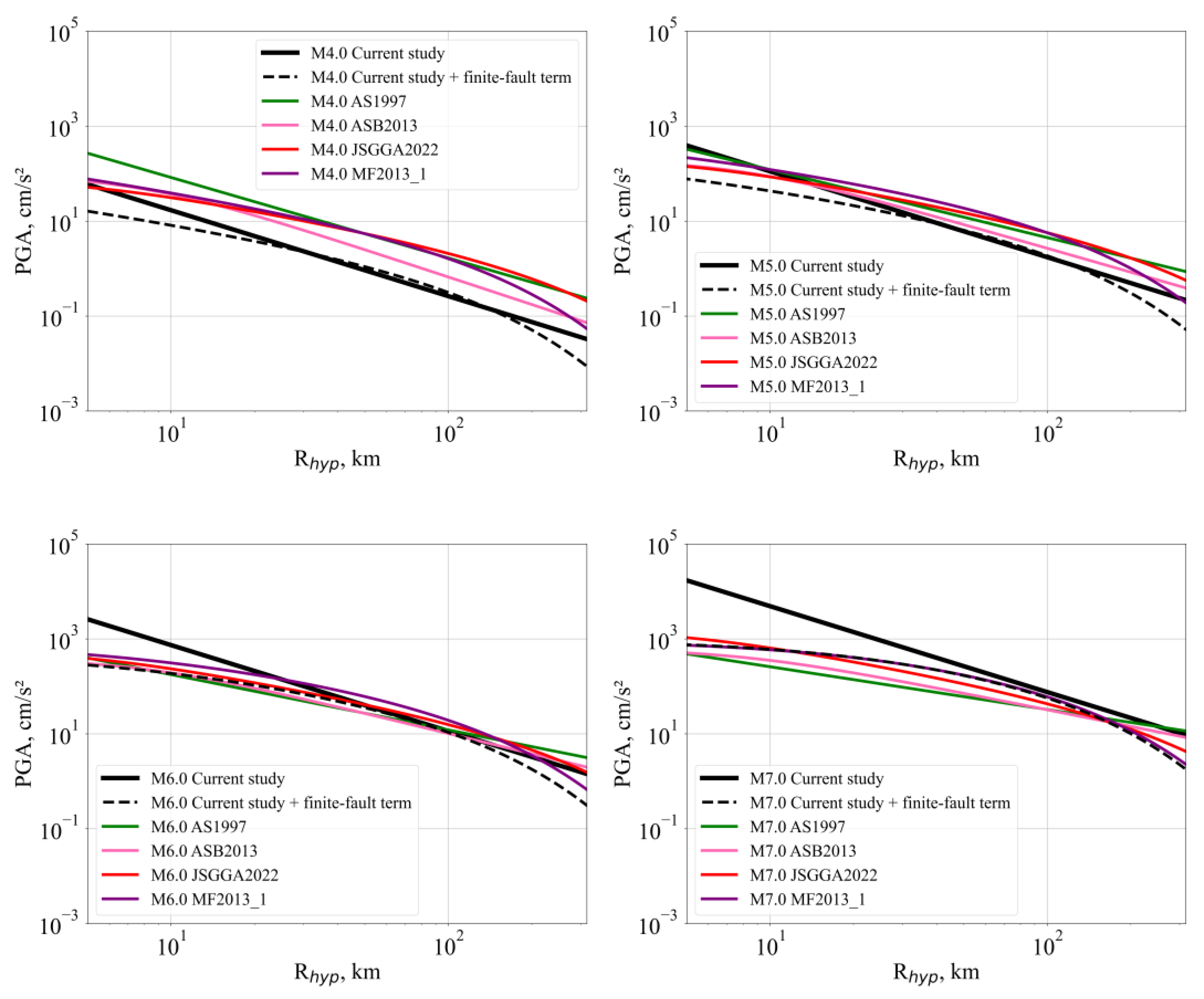
4.2. Comparison of GMPEs and Finite-Fault Effects

In our study, we compared the resulting equation for PGA with several global and regional models for the crustal seismicity (see Figure 10). The four GMPEs were: AS1997 [49], ASB2013 [47], JSGGA2022 [50], and MF2013_1 [29]. The comparisons are presented on each panel corresponding to the earthquake magnitudes M 4, M 5.0, M 6, and M 7. Attenuation equations were reduced to VS30 = 350 m/s and the reverse faulting mechanism. Models JSGGA2022 and ASB2013 were developed using the Rhyp metric, whereas other GMPEs used Rrup and Rjb. Although GMPEs are guided with different uses in distance metrics, this does not significantly affect the overall results due to the point-source approximation for the considered magnitude range.

Figure 10 presents the model-to-model variability caused by regional differences. As can be observed in these figures, the simple point-source model developed in the current study did not extrapolate well to magnitudes of M ≥ 5 at short distances that often control seismic hazard outcomes. To be useful for seismic hazard applications, the GMPE needs to perform extrapolations in a reasonable manner. The finite-fault term added to the distance metric in Equation (4) was one way to force the point-source model to perform extrapolations properly. We imported this term from the model MF2013_1. The MF2013_1 model used for crustal seismicity in Japan was developed in the form of a geometric representation of GMPE. This means that the geometrical spreading term presented in Equation (4) was taken as $k$ = 1. Therefore, we added an additional term to Equation (4). The hybrid model is presently formulated as

$$\lg PGA=a\times \mathrm{M}-\lg \left(R+d\times {10}^{e\times M}\right)-b\times R+c\pm \sigma ,$$

(40)

where $d$ and $e$ are the constants $d$ = 0.006875 and $e$ = 0.5.

The parameters of the developed attenuation model in the geometric representation are presented in Table 3c. The corresponding illustration is presented in Figure 10.

The lineament-domain source model was used in the seismic hazard assessments conducted on Sakhalin Island. The maximum magnitude for area sources did not exceed Mw 6. For such seismic sources, one can use the regional attenuation Equation (40), while for extended line sources the global models should be applied.

Figure 11 presents a comparison of the attenuation curves with the data normalized to Mw 7.0. The observed data were normalized as follows:

$$\lg {obs}^{\prime }=\lg obs+\lg pre\left(\mathrm{M}\mathrm{w}=7\right)-\lg pre\left(\mathrm{M}\right),$$

(41)

where ${obs}^{\prime }$ is the normalized data, $obs$ is the observed data, $pre\left(\mathrm{M}\right)$ is the predicted value by Equation (40) for identical parameters with observed data, and $pre\left(\mathrm{M}\mathrm{w}=7\right)$ is the predicted value for Mw 7.

The PGA values at the near-source distances were close to the flat level at approximately 800 cm/s² (Figure 11). The PGA values converted from macroseismic intensity (https://earthquake.usgs.gov/earthquakes/eventpage/usp0006y50/shakemap/stations?source=atlas&code=usp0006y50, accessed on 7 June 2022) for the catastrophic 1995 Neftegorsk earthquake (Mw 7.1) fit the prediction model well. The hypocentral distance was replaced by the rupture distance.

4.3. Selection of Point-Source Distance Metrics

The choice of distance metrics in ground motion attenuation models is frequently discussed in the scientific community (e.g., https://usgs.github.io/shakemap/manual3_5/tg_processing.html, accessed on 1 June 2022). The distance metrics Rrup and Rjb are most commonly used as the characteristic distance between the finite source and the site for seismic hazard assessments. That is why developers of GMPEs often select the abovementioned distance metrics. However, to rapidly generate shaking maps, hypocentral (or epicentral) distances are preferred in the research, since the finite-source characteristics are reported by seismological data centers more slowly than the hypocenter parameters.

An analysis of regional and global empirical attenuation relationships (http://www.gmpe.org.uk, accessed on 1 June 2022) indicates the lack of Rhyp-based GMPEs in active crustal regions. Apparently, the only exception to this practice is the ASB2013 model [47], developed by the authors specifically for European countries, which can be classified as a region with a stable continental crust. In this model, the Rhyp distance metric, as well as Rjb and Rrup, were used. Therefore, the model developed in the current study concerning the empirical attenuation relationships based on the Rhyp distance metric can be used in early warning systems (e.g., [51]) to perform an accurate prediction of the ground shaking level in the study area.

5. Conclusions

1. Empirical attenuation relations for multiple ground motion intensity measures (PGA, PGV, I_a, FIV3, CII, and MFAS) were developed in the current study. Some of these factors referred to low-frequency metrics (e.g., FIV3), while the Arias (I_a) and spectral (MFAS) intensities were characteristic of high-frequency incoherent radiation, according to the multi-asperity source model. A recorded strong motion dataset was used in our study, making the GMPEs applicable to an earthquake magnitude range of 4–6 and a distance of up to 150 km. The hypocentral distance was used as a basic distance metric. The target area was the transition zone from the Pacific Ocean to the continental regions of Russia.

2. We proposed a GMPE corresponding to the simple point-source model with the physical value of geometrical spreading for the prediction of PGA in Sakhalin Island and the surrounding shelf. The applicability of the presented model was strictly bound to the magnitude range of 4–6. The reference V_S30 took a value of 350 m/s. Site and finite-fault terms describing the PGA model in Japan were preferred for use in the present GMPE.

3. The attenuation relations based on the MFAS spectral metric, as well as a filtered incremental velocity of FIV3(0.01), were characterized by the smallest scattering pattern among the considered ground motion measures.

4. For the first time, an analytical representation of the Arias intensity (I_a) was obtained in the framework of a fragmented source model with asperities, which are sub-sources of high-frequency radiation. This allowed us to use this metric for estimating the average stress drop on asperities occurring in the target region.

5. The average stress drop on asperities for the examined earthquakes was approximately 13.4 MPa, and the ratio of the total rupture area to the combined area of asperity was 0.22, which is generally similar to the estimates for crustal earthquakes occurring in Japan.

6. The modified I_a metrics proposed in the current study were based on the prefiltering of acceleration records with high-pass filters. It was shown that the coefficient associated with the magnitude term in the GMPE decreased and tended towards unity when the cut-off frequency of the filter increased. We attributed the observed deviations from the theory to a violation of the source model, according to which the amplitude spectra decayed with the frequency according to the ω²-law.

7. When the cut-off frequency of the HP filter increased, an increase in the statistical scattering in the attenuation equation for the modified I_a metric was evident. This was explained in terms of the kappa attenuation parameter.

8. A modified I_a(3) metric was proposed to calibrate the new magnitude scale associated with the acceleration source spectrum level in the high-frequency range.

References

1. Guaman, J.; Kirkner, D.; Kurama, Y. Empirical ground motion attenuation relationships for maximum incremental velocity. In Proceedings of the 9th US National and 10th Canadian Conference on Earthquake Engineering 2010, Including Papers from the 4th International Tsunami Symposium, Toronto, ON, Canada, 25 July 2010. [Google Scholar]
2. Earthquake Research Committee. Seismic Activity in Japan: Regional Perspectives on the Characteristics of Destructive Earthquakes; Science and Technology Agency: Tokyo, Japan, 1998. [Google Scholar]
3. Kramer, S.L.; Mitchell, R.A. Ground motion intensity measures for liquefaction hazard evaluation. Earthq. Spectra 2006, 22, 413–438. [Google Scholar] [CrossRef]
4. Campbell, K.W.; Bozorgnia, Y. Cumulative absolute velocity (CAV) and seismic intensity based on the PEER-NGA database. Earthq. Spectra 2012, 28, 457–485. [Google Scholar] [CrossRef]
5. Ji, D.; Liu, J.; Wen, W.; Zhai, C.; Wang, W.; Katsanos, E.I. Prediction of Cumulative Absolute Velocity Based on Refined Second-order Deep Neural Network. J. Earthq. Eng. 2021, 26, 8021–8040. [Google Scholar] [CrossRef]
6. Bullock, Z.; Dashti, S.; Liel, A.; Porter, K.; Karimi, Z.; Bradley, B. Ground-motion prediction equations for Arias intensity, cumulative absolute velocity, and peak incremental ground velocity for rock sites in different tectonic environments. Bull. Seismol. Soc. Am. 2017, 107, 2293–2309. [Google Scholar] [CrossRef]
7. Jampole, E.; Miranda, E.; Deierlein, G. Effective incremental ground velocity: An IM to estimate sliding isolation displacement. In Proceedings of the 11th National Conference on Earthquake Engineering, NCEE 2018: Integrating Science, Engineering, and Policy, Los Angeles, CA, USA, 25–29 June 2018. [Google Scholar]
8. Dávalos, H.; Miranda, E. Filtered incremental velocity: A novel approach in intensity measures for seismic collapse estimation. Earthq. Eng. Struct. Dyn. 2019, 48, 1384–1405. [Google Scholar] [CrossRef]
9. Dávalos, H.; Heresi, P.; Miranda, E. A ground motion prediction equation for filtered incremental velocity, FIV3. Soil Dyn. Earthq. Eng. 2020, 139, 1384–1405. [Google Scholar] [CrossRef]
10. Wilson, R.C. Relation of Arias Intensity to Magnitude and Distance in California; US Geological Survey: Reston, VA, USA, 1993. [CrossRef]
11. Stafford, P.J.; Berrill, J.B.; Pettinga, J.R. New predictive equations for Arias intensity from crustal earthquakes in New Zealand. J. Seismol. 2009, 13, 31–52. [Google Scholar] [CrossRef] [Green Version]
12. Keefer, D.K.; Wilson, R.C. Predicting earthquake-induced landslides, with emphasis on arid and semi-arid environments. Landslides A Semi-Arid. Environ. 1989, 2, 118–149. [Google Scholar]
13. Li, X.; Xu, W.; Gao, M. Characteristics of Arias intensity and Newmark displacement of strong ground motion in Lushan earthquake. Acta. Seismol. Sin. 2021, 43, 768–786. [Google Scholar] [CrossRef]
14. Chernov, Y.K. Strong Ground Motion and Quantitative Assessment of Seismic Hazard; Fan Publishing House: Tashkent, Uzbekistan, 1989. [Google Scholar]
15. Sokolov, V.Y. Seismic intensity and Fourier acceleration spectra: Revised relationship. Earthq. Spectra 2002, 18, 161–187. [Google Scholar] [CrossRef]
16. Kotha, S.R.; Bindi, D.; Cotton, F. A regionally adaptable ground-motion model for fourier amplitude spectra of shallow crustal earthquakes in Europe. Bull. Earthq. Eng. 2022, 20, 711–740. [Google Scholar] [CrossRef]
17. Vemula, S.; Raghukanth, S.T.G. Generation of a Response Spectrum from a Fourier Spectrum Using a Recurrent Neural Network: Application to New Zealand. Pure Appl. Geophys. 2022, 179, 2797–2816. [Google Scholar] [CrossRef]
18. Irikura, K.; Miyake, H. Recipe for predicting strong ground motion from crustal earthquake scenarios. Pure Appl. Geophys. 2011, 168, 85–104. [Google Scholar] [CrossRef] [Green Version]
19. Feng, T.; Meng, L. A High-Frequency Distance Metric in Ground-Motion Prediction Equations Based on Seismic Array Backprojections. Geophys. Res. Lett. 2018, 45, 11–612. [Google Scholar] [CrossRef]
20. Ito, C.; Takahashi, H.; Ohzono, M. Estimation of convergence boundary location and velocity between tectonic plates in northern Hokkaido inferred by GNSS velocity data. Earth Planets Space 2019, 71, 86. [Google Scholar] [CrossRef] [Green Version]
21. García, D.; Wald, D.J.; Hearne, M.G. A global earthquake discrimination scheme to optimize ground-motion prediction equation selection. Bull. Seismol. Soc. Am. 2012, 102, 185–203. [Google Scholar] [CrossRef]
22. Konovalov, A.V.; Nagornyh, T.V.; Safonov, D.A. Resent study of earthquake source mechanisms in Sakhalin. In Vladivostok: Dal’nauka; Kozhurin, A.I., Ed.; Dal’nauka: Vladivostok, Russia, 2014; 252p. [Google Scholar]
23. Konovalov, A.V.; Sychev, A.S. A calibration curve of local magnitude and intermagnitude relations for northern Sakhalin. J. Volcanol. Seismol. 2014, 8, 390–400. [Google Scholar] [CrossRef]
24. Gusev, A.A.; Mel’nikova, B.N. Relations between magnitudes—World average and for Kamchatka. Vulkanol Seism. 1990, 6, 55–63. [Google Scholar]
25. Federal Emergency Management Agency (FEMA), Edition NEHRP Recommended Provisions for Seismic Regulations for New Buildings and Other Structures, Part 1: Provisions (FEMA 302). 1997. Available online: http://www.ce.memphis.edu/7137/PDFs/fema302a.pdf (accessed on 16 August 2022).
26. Wald, D.J.; Quitoriano, V.; Dengler, L.A.; Dewey, J.W. Utilization of the Internet for rapid community intensity maps. Seismol. Res. Lett. 1999, 70, 680–697. [Google Scholar] [CrossRef]
27. Konovalov, A.V.; Stepnov, A.A.; Bogdanov, E.S.; Dmitrienko, R.Y.; Orlin, I.D.; Sychev, A.S.; Gavrilov, A.V.; Manaychev, K.A.; Tsoy, A.T.; Stepnova, Y.A. New Tools for Rapid Assessment of Felt Reports and a Case Study on Sakhalin Island. Seism. Instruments. 2022, 58, 676–693. [Google Scholar] [CrossRef]
28. Si, H.; Midorikawa, S. New Attenuation Relationships for Peak Ground Acceleration and Velocity Considering Effects of Fault Type and Site Condition. J. Struct. Constr. Eng. 1999, 64, 63–70. [Google Scholar] [CrossRef] [Green Version]
29. Morikawa, N.; Fujiwara, H. A new ground motion prediction equation for Japan applicable up to M9 mega-earthquake. J. Disaster Res. 2013, 8, 878–888. [Google Scholar] [CrossRef]
30. Fukushima, Y.; Tanaka, T. A new attenuation relation for peak horizontal acceleration of strong earthquake ground motion in Japan. Bull. Seismol. Soc. Am. 1990, 80, 757–783. [Google Scholar] [CrossRef]
31. Kanno, T.; Narita, A.; Morikawa, N.; Fujiwara, H.; Fukushima, Y. A New Attenuation Relation for Strong Ground Motion in Japan Based on Recorded Data. Bull. Seismol. Soc. Am. 2006, 96, 879–897. [Google Scholar] [CrossRef]
32. Joyner, W.B.; Boore, D.M. Peak horizontal acceleration and velocity from strong-motion records including records from the 1979 imperial valley, California, earthquake. Bull. Seismol. Soc. Am. 1981, 71, 2011–2038. [Google Scholar] [CrossRef]
33. Hanks, T.C.; McGuire, R.K. The character of high-frequency strong ground motion. Bull. Seismol. Soc. Am. 1981, 71, 2071–2095. [Google Scholar] [CrossRef]
34. Madariaga, R. High-frequency radiation from crack (stress drop) models of earthquake faulting. Geophys. J. Int. 1977, 51, 625–651. [Google Scholar] [CrossRef] [Green Version]
35. Gusev, A.A. Multiasperity fault model and the nature of short-period subsources. Pure Appl. Geophys. 1989, 130, 635–660. [Google Scholar] [CrossRef]
36. Gusev, A.A. Random kinematics of unbounded earthquake rupture propagation simulated using a cellular model. Geophys. J. Int. 2018, 215, 924–941. [Google Scholar] [CrossRef]
37. Boore, D.M. Simulation of Ground Motion Using the Stochastic Method. Pure Appl. Geophys. 2003, 160, 635–676. [Google Scholar] [CrossRef] [Green Version]
38. Bansal, B.K.; Singh, S.K.; Suresh, G.; Mittal, H. A source and ground motion study of earthquakes in and near Delhi (the National Capital Region), India. Nat. Hazards 2022, 111, 1885–1905. [Google Scholar] [CrossRef]
39. Konovalov, A.V.; Sychev, A.S.; Solov’ev, V.N. Mass estimates of the scalar seismic moments of small earthquake foci on southern Sakhalin. Russ. J. Pacific. Geol. 2011, 5, 225–233. [Google Scholar] [CrossRef]
40. Kosuga, M. Dependence of Coda Q on Frequency and Lapse Time in the Western Nagano Region, Central Japan. J. Phys. Earth 1992, 40, 421–445. [Google Scholar] [CrossRef]
41. Kostrov, B.V. Mechanics of Tectonic Earthquake Source; Nauka: Moscow, Russia, 1975; 176p. [Google Scholar]
42. Hanks, T.C.; Kanamori, H. A moment magnitude scale. J. Geophys. Res. B Solid. Earth 1979, 84, 2348–2350. [Google Scholar] [CrossRef]
43. Xu, B.; Rathje, E.M.; Hashash, Y.M.A.; Stewart, J.P.; Campbell, K.W.; Silva, W.J. k0 for soil sites: Observations from KiK-net sites and their use in constraining small-strain damping profiles for site response analysis. Earthq. Spectra 2020, 36, 111–137. [Google Scholar] [CrossRef]
44. Satoh, T.; Okazaki, A. Relation Between Stress Drops and Depths of Strong Motion Generation Areas Based on Previous Broadband Source Models for Crustal Earthquakes in Japan. In Earthquakes, Tsunamis and Nuclear Risks, Predicition and Assessment beyond the Fukushima Accident, Part II; Kamae, K., Ed.; OAPEN Library: Hague, The Netherlands, 2016; pp. 77–85. [Google Scholar] [CrossRef] [Green Version]
45. Dan, K.; Watanabe, M.; Sato, T.; Ishii, T. Short-period source spectra inferred from variable-slip rupture models and modeling of earthquake faults for strong motion prediction by semi-empirical method. J. Struct. Constr. Eng. 2001, 66, 51–62. [Google Scholar] [CrossRef] [Green Version]
46. González, J.; Irikura, K. Source Characterization of Mexican Subduction Earthquakes from Acceleration Source Spectra for the Prediction of Strong Ground Motions. Bull. Seismol. Soc. Am. 2007, 97, 1960–1969. [Google Scholar] [CrossRef]
47. Akkar, S.; Sandıkkaya, M.A.; Bommer, J.J. Empirical ground-motion models for point- and extended-source crustal earthquake scenarios in Europe and the Middle East. Bull. Earthq. Eng. 2014, 12, 359–387. [Google Scholar] [CrossRef] [Green Version]
48. Yao, Q.; Wang, D.; Fang, L.; Mori, J. Rapid Estimation of Magnitudes of Large Damaging Earthquakes in and around Japan Using Dense Seismic Stations in China. Bull. Seismol. Soc. Am. 2019, 109, 2545–2555. [Google Scholar] [CrossRef]
49. Abrahamson, N.A.; Silva, W.J. Empirical response spectral attenuation relations for shallow crustal earthquakes. Seismol. Res. Lett. 1997, 68, 94–109. [Google Scholar] [CrossRef] [Green Version]
50. Jorjiashvili, N.; Shengelia, I.; Godoladze, T.; Gunia, I.; Akubardia, D. Ground motion prediction equations based on shallow crustal earthquakes in Georgia and the surrounding Caucasus. Earthq. Sci. 2022, 35, 497–509. [Google Scholar] [CrossRef]
51. Allen, R.M.; Melgar, D. Earthquake Early Warning: Advances, Scientific Challenges, and Societal Needs. Annu. Rev. Earth Planet Sci. 2019, 47, 361–388. [Google Scholar] [CrossRef] [Green Version]
Figure 1. Geographical location of the study area, major seismic events, tectonic boundaries, active faults, instrumental sites, and epicenters of the earthquakes considered in the study, AM—Amurian Plate, OK—Okhotsk Plate, black arrows indicate the principal axes of compression.
Geosciences 13 00201 g001
Figure 2. Magnitude versus distance distribution of the strong motion database considered in the study.
Geosciences 13 00201 g002
Figure 3. Accelerograms (horizontal components NS and EW) and transformed records of the 18 April 2021 shallow earthquake (ML 4.5). The hypocentral distance is 9.5 km. The ground shaking measures are marked by green circles. Red dotted lines correspond to 5% and 95% signal duration values.
Geosciences 13 00201 g003
Figure 4. The acceleration spectrum ( N S 2 + E W 2 ) of the seismic records illustrated in Figure 3. The ground shaking measure is marked by a green circle.
Geosciences 13 00201 g004
Figure 5. Parameter Ψ as a function of λ following numerical integration.
Geosciences 13 00201 g005
Figure 6. Instrumental and macroseismic measures (open circles), and the best attenuation curves (solid lines) in the statistical representation corresponding to them. Empirical attenuation curves are based on the moment magnitude (Mw).
Geosciences 13 00201 g006
Figure 7. Stress drops on asperities ( τ ) and the whole fault ( σ ) as a function of the filling factor k f .
Geosciences 13 00201 g007
Figure 8. Empirical relationship between the moment magnitude (Mw) and acceleration source spectral level (A) for different regions and tectonic types, deviation by Dan et al., 2001 [45].
Geosciences 13 00201 g008
Figure 9. Distribution of frequencies corresponding to the MFAS spectral metric.
Geosciences 13 00201 g009
Figure 10. Distance attenuation values of PGA for a comparison of the developed GMPEs with the global and regional attenuation equations. A description of the models is presented in the text.
Geosciences 13 00201 g010
Figure 11. Distance attenuation values of PGA for data normalized to Mw 7. Solid and broken lines represent the attenuation curve and corresponding standard deviation, respectively.
Geosciences 13 00201 g011