Impact of Extreme Weather Events on Aboveground Net Primary Productivity and Sheep Production in the Magellan Region, Southernmost Chilean Patagonia

 ,
,  ,
,
Abstract
:1. Introduction
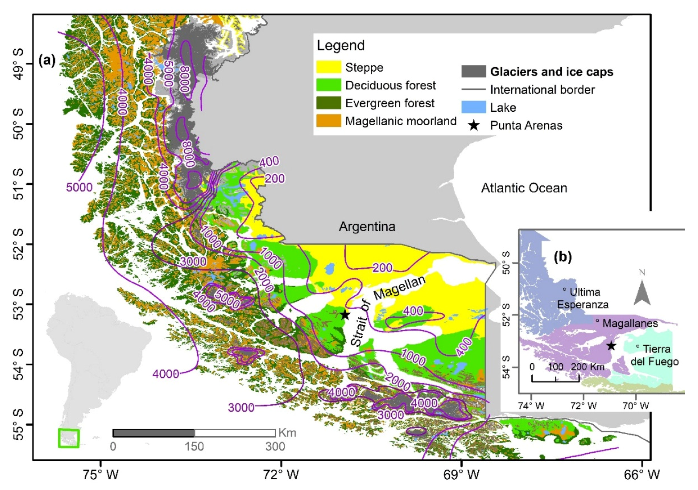
2. Study Area

3. Methods
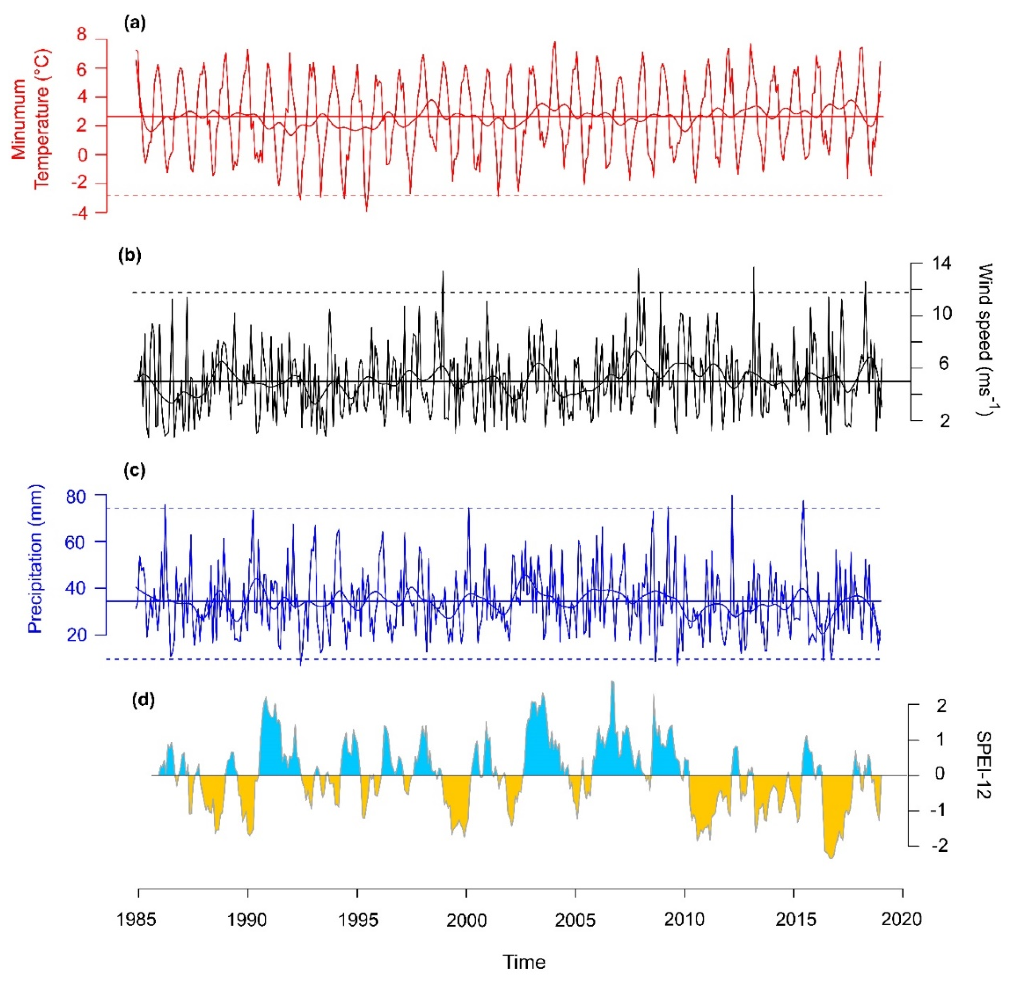
3.1. Regional Climate Variability
3.2. Relationship between Climate Variability and Vegetation Cover
3.3. Relationship between Climate Variability and Sheep Production
3.4. Impact of Extreme Event on Aboveground Net Primary Productivity and Sheep Production
4. Results
4.1. Recent Changes in Regional Climate Variability
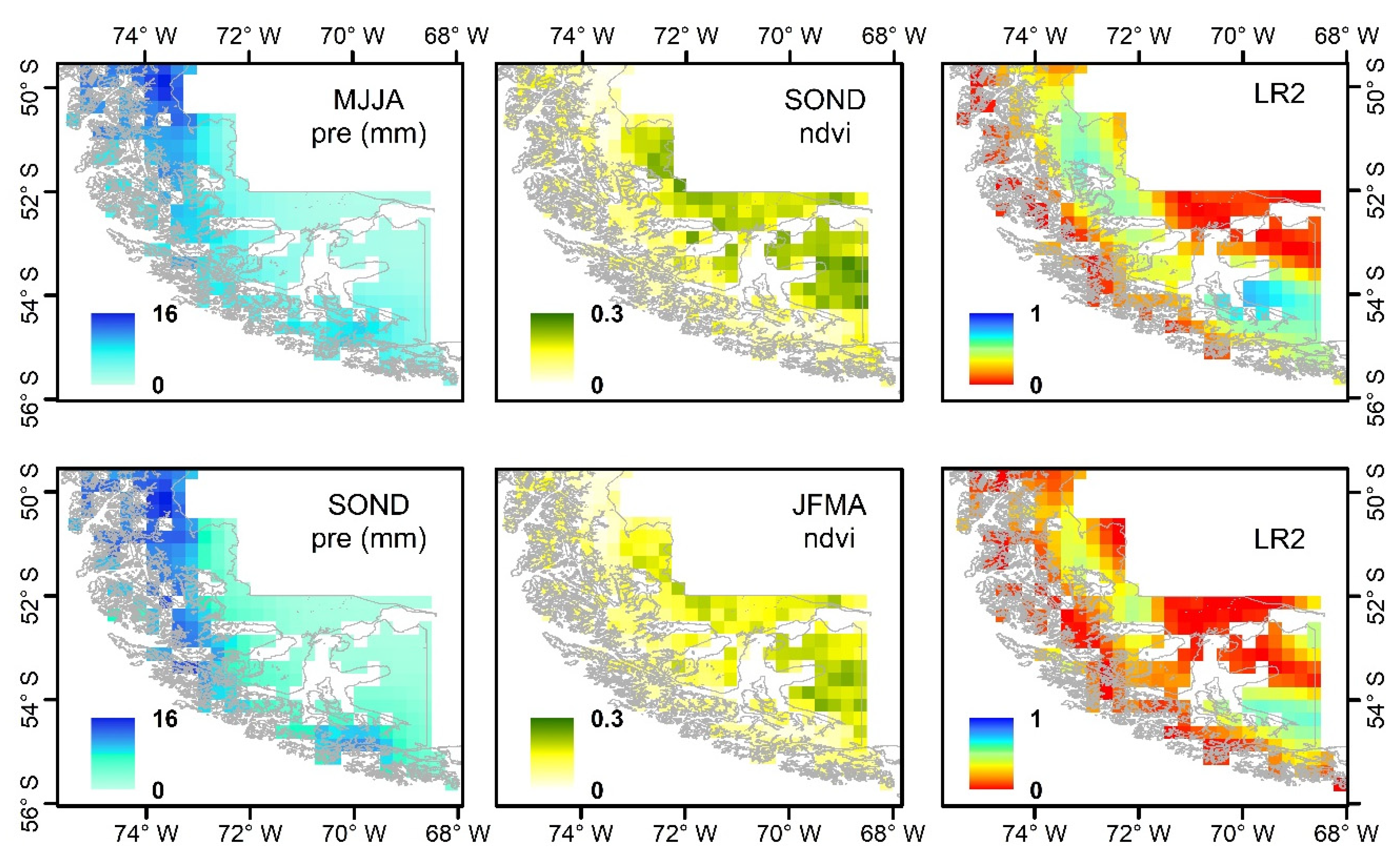
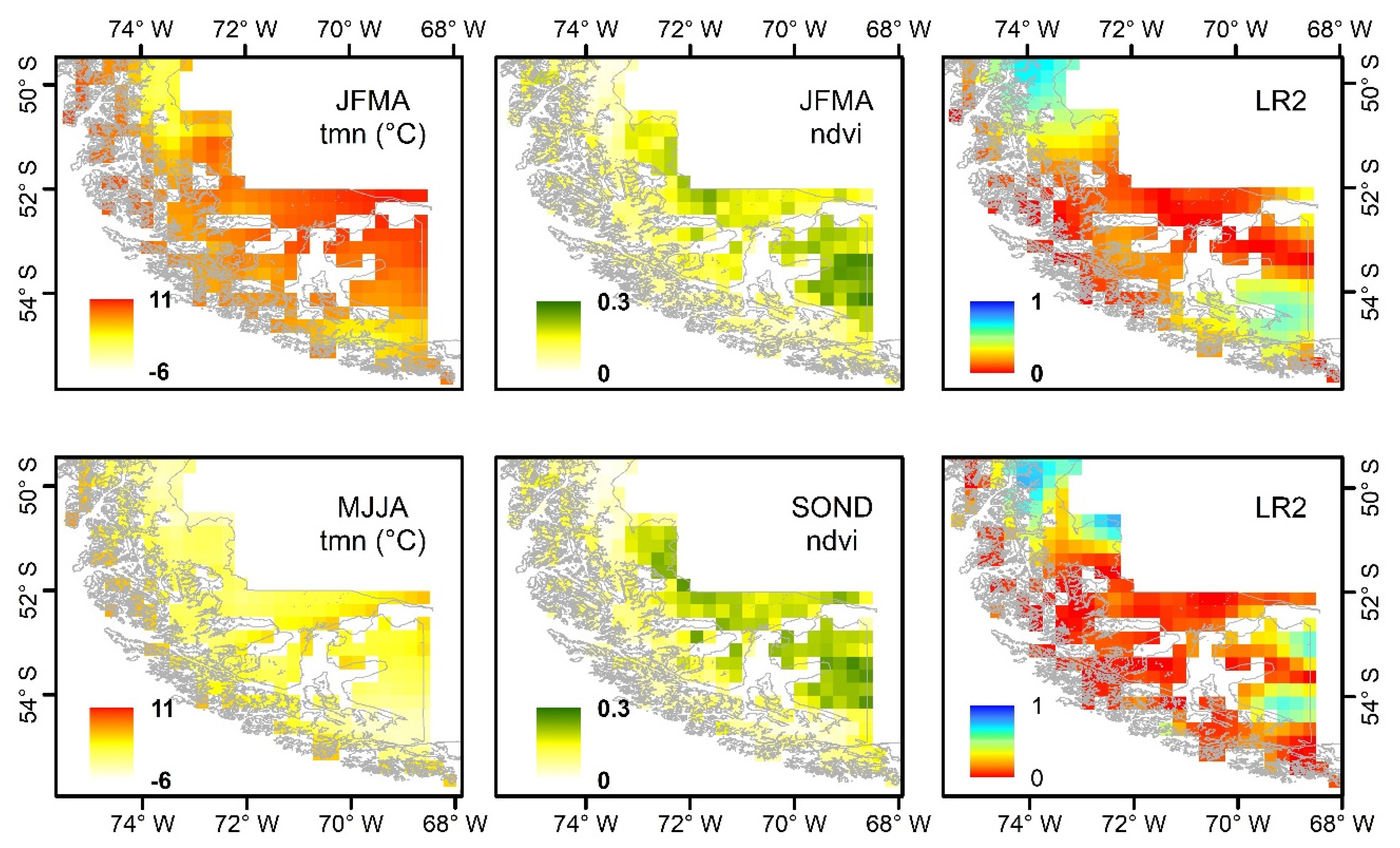
4.2. Relationship between Climate Variability and Seasonal Vegetation Cover
4.3. Relationship between Sheep Production and Climate Variability
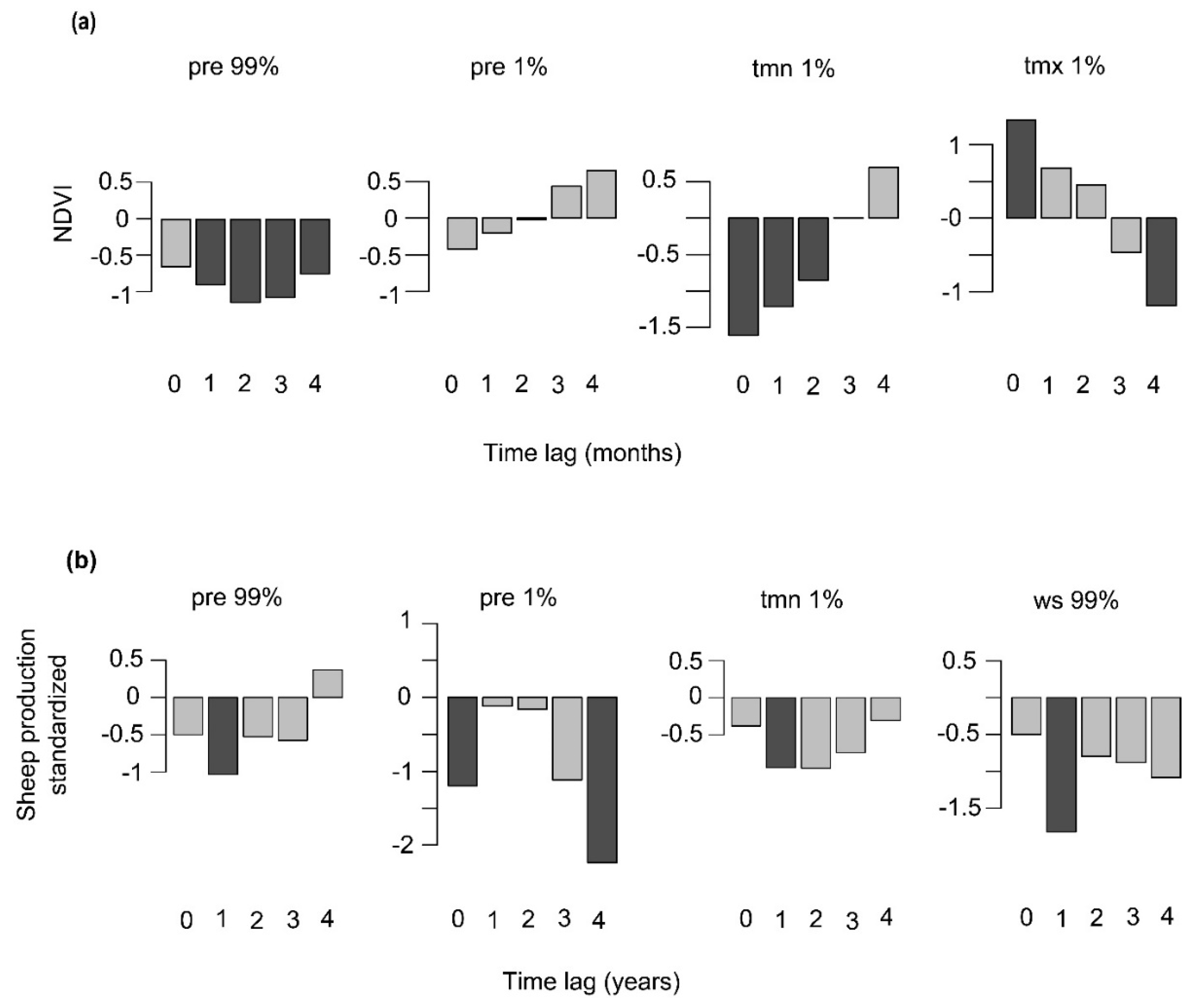
4.4. Impact of Extreme Events on Above Net Primary Productivity and Sheep Production
5. Discussion
5.1. Extreme Weather Events, Net Primary Productivity and Sheep Production
5.2. Sheep Production, Climate and Aboveground Net Primary Productivity (ANPP)
6. Conclusions
Author Contributions
Funding
Acknowledgments
Conflicts of Interest
References
- Covacevich, N.; Ruz, E. Praderas en la zona austral: XII Región (Magallanes). In Praderas Para Chile, 2nd ed.; Ruiz, I., Ed.; Instituto de Investigaciones Agropecuarias: Santiago, Chile, 1988; pp. 640–655. [Google Scholar]
- INE-Odepa. Enfoque Estadístico: VII Censo Nacional Agropecuario y Forestal; Ministerio de Agricultura: Santiago, Chile, 2007. [Google Scholar]
- Odepa. Región de Magallanes y la Antártica Chilena, Informativo Regional; Ministerio de Agricultura: Santiago, Chile, 2019. [Google Scholar]
- Pisano, E. Fitogeografía de Fuego-Patagonia chilena. I. Comunidades vegetales entre las latitudes 52 y 56° S. Ans. Inst. Pat. (Chile) 1977, 8, 121–250. [Google Scholar]
- González-Reyes, A.; Aravena, J.C.; Muñoz, A.; Soto-Rogel, P.; Aguilera-Betti, I.; Toledo-Guerrero, I. Variabilidad de la precipitación en la ciudad de Punta Arenas, Chile, desde principios del siglo XX. Ans. Inst. Pat. (Chile) 2017, 45, 31–44. [Google Scholar] [CrossRef] [Green Version]
- Carrasco, J. Decadal Changes in the Near-Surface Air Temperature in the Western Side of the Antarctic Peninsula. Atmos. Clim. Sci. (ACS) 2013, 3, 275–281. [Google Scholar] [CrossRef] [Green Version]
- IPCC. Climate Change 2013: The Physical Science Basis. Contribution of Working Group I to the Fifth Assessment Report of the Intergovernmental Panel on Climate Change; Cambridge University Press: Cambridge, UK; New York, UY, USA, 2013; p. 1535. [Google Scholar]
- Smith, P.; Bustamante, M.; Ahammad, H. Agriculture, forestry and other land use (AFOLU). In Climate Change 2014: Mitigation of Climate Change. Contribution of Working Group III to the Fifth Assessment Report of the Intergovernmental Panel on Climate Change; Edenhofer, O., Pichs-Madruga, R., Sokona, Y., Eds.; Cambridge University Press: Cambridge, UK; New York, NY, USA, 2014; pp. 829–833. [Google Scholar]
- Beniston, M.; Stephenson, D.B. Extreme climatic events and their evolution under changing climatic conditions. Glob. Planet. Chang. 2004, 44, 1–9. [Google Scholar] [CrossRef] [Green Version]
- Endlicher, W.; Santana, A. El clima del sur de la Patagonia y sus aspectos ecológicos. Un siglo de mediciones climatológicas en Punta Arenas. Ans Inst. Pat. Ser. Cs. Nat. (Chile) 1988, 18, 59–86. [Google Scholar]
- Endlicher, W.; Santana, A. El invierno de 1995: Un fenómeno climático muy severo en la Patagonia austral. Ans Inst. Pat. Ser. Cs. Nat. (Chile) 1997, 25, 77–88. [Google Scholar]
- Butorovic, N. Resumen Meteorológico año 2015 Estación “Jorge C. Schythe” (53°08′S; 70°53′O; 6 msnm). Ans. Inst. Pat. (Chile) 2018, 44, 1–10. [Google Scholar] [CrossRef] [Green Version]
- Meza, L. Adaptación del Sector Silvoagropecuario a la Variabilidad y el Cambio Climático en la Región de Magallanes y de la Antártica Chilena: Experiencia de Cooperación en la Planificación Regional la Planificación Regional; FAO: Santiago, Chile, 2014. [Google Scholar]
- Centro de Ciencia del Clima y la Resiliencia (CR)2. Available online: http://www.cr2.cl/ (accessed on 25 June 2020).
- Gaitán, J.J.; Bran, D.; Oliva, G.; Maestre, F.T.; Aguiar, M.R.; Jobbágy, E.; Buono, G.; Ferrante, D.; Nakamatsu, V.; Ciari, G.; et al. Plant species richness and shrub cover attenuate drought effects on ecosystem functioning across Patagonian rangelands. Biol. Lett. 2014, 10, 20140673. [Google Scholar] [CrossRef] [Green Version]
- Covacevich, N. Guía de Manejo de Coironales: Bases Para el Planteamiento de la Estancia; Instituto de Investigaciones Agropecuarias: Punta Arenas, Chile, 2001. [Google Scholar]
- Villa, M.; Opazo, S.; Moraga, C.; Muñoz-Arriagada, R.; Radic, S. Patterns of vegetation and climatic conditions derived from satellite images relevant for sub-antarctic rangeland management. Rangel. Ecol. Manag. 2020, in press. [Google Scholar] [CrossRef]
- Graetz, R.D. Desertification: A tale of two feedbacks. In Ecosystem Experiments; Mooney, H.A., Medina, E., Schindler, D., Schulze, E.D., Walker, B.H., Eds.; Wiley: Chichester, UK, 1991; pp. 59–87. [Google Scholar]
- Jobbágy, E.; Sala, O. Control of grass and shrub aboveground production in the Patagonia steppe. Ecol. Appl. 2000, 10, 541–549. [Google Scholar] [CrossRef]
- Jobbágy, E.; Sala, O.; Paruelo, J.M. Patterns and controls of primary production in the Patagonian steppe: A remote sensing approach. Ecology 2002, 83, 307–319. [Google Scholar] [CrossRef] [Green Version]
- Sala, O.; Gherardi, L.; Reichmann, L.; Jobbágy, E.; Peters, D. Legacies of precipitation fluctuations on primary production: Theory and data synthesis. Phil. Trans. R. Soc. B 2012, 367, 3135–3144. [Google Scholar] [CrossRef] [PubMed]
- Peri, P.; Rosas, Y.; Ladd, B.; Díaz-Delgado, R.M.; Martínez Pastur, G. Carbon Footprint of Lamb and Wool Production at Farm Gate and the Regional Scale in Southern Patagonia. Sustainability 2020, 12, 3077. [Google Scholar] [CrossRef] [Green Version]
- Ruz, E. Explotación Agrícola de Praderas Naturales: El Caso de Magallanes. In Anuario Corriedale (Punta Arenas); Asociación Chilena de Criadores: Punta Arenas, Chile, 1987; pp. 87–94. [Google Scholar]
- Covacevich, N. Manejo Sustentable de las Praderas Naturales de Magallanes. La Situación Actual de los Recursos Forrajeros; Instituto de Investigaciones Agropecuarias: Punta Arenas, Chile, 2006. [Google Scholar]
- Latorre, E.; Tapia, D.; Bennewitz, R.; Cancino, L.; Rivera, A.; Toscón, M.T.; Saldivia, A. Agenda de Innovación Estratégica Ovina: Carne-Lana Región de Magallanes y Antártica Chilena; Secretaria Regional Ministerial de Agricultura Región de Magallanes y Antártica: Punta Arenas, Chile, 2015. [Google Scholar]
- Strauch, O.; Lira, R. Bases Para la Producción ovina en Magallanes; Instituto de Investigaciones Agropecuarias; Centro Regional de Investigación: Punta Arenas, Chile, 2012. [Google Scholar]
- Carrasco, J.; Casassa, G.; Rivera, A. Meteorological and climatological. In The Patagonian Icefields. A Unique Natural Laboratory for Environmental and Climate; Casassa, G., Sepúlveda, F.V., Sinclair, R.M., Eds.; Kluwer Academic/Plenum: New York, NY, USA, 2002; pp. 29–42. [Google Scholar]
- Aravena, J.C.; Luckman, B.H. Spatio-temporal rainfall patterns in Southern South America. Int. J. Climatol. 2009, 29, 2106–2120. [Google Scholar] [CrossRef]
- Soto-Rogel, P.; Aravena, J.C. Potencial dendroclimático de Nothofagus betuloides en la Cordillera de Darwin, Tierra del Fuego. Bosque (Valdivia) 2017, 38, 155–168. [Google Scholar] [CrossRef] [Green Version]
- Luebert, F.; Pliscoff, P. Sinopsis Bioclimática y Vegetacional de Chile; Universitaria: Santiago, Chile, 2018; p. 384. [Google Scholar]
- Infraestructura de Datos Geoespaciales de Chile (IDE). Available online: http://www.ide.cl/ (accessed on 25 June 2020).
- Harris, I.; Jones, P.D.; Osborne, T.J.; Lister, D.H. Updated high-resolution grids of monthly climatic observations—the CRU TS3.10 Dataset. Int. J. Climatol. 2014, 34, 623–642. [Google Scholar] [CrossRef] [Green Version]
- Beguería, S.; Vicente-Serrano, S. SPEI: An R Package for Calculation of the Standardised Precipitation-Evapotranspiration Index. 2017. Available online: https://cran.r-project.org/web/packages/SPEI/SPEI.pdf. (accessed on 15 March 2020).
- R Core Team. R: A language and environment for statistical computing. R Found. Stat. Comput. 2019. Available online: www.R-project.org/ (accessed on 1 March 2020).
- Vermote, E. NOAA Climate Data Record (CDR) of AVHRR Normalized Difference. Natl. Cent. Environ. Inf. 2019. [Google Scholar] [CrossRef]
- Tucker, C.J.; Sellers, P.J. Satellite remote sensing for primary production. Int. J. Remote Sens. 1986, 7, 1395–1416. [Google Scholar] [CrossRef]
- Paruelo, J.M.; Epstein, H.E.; Lauenroth, W.K.; Burke, I.C. ANPP estimates from NDVI for the Central Grassland Region of the United States. Ecology 1997, 78, 953–958. [Google Scholar] [CrossRef]
- Dee, D.P.; Uppala, S.M.; Simmons, A.J.; Berrisford, P.; Poli, P.; Kobayashi, S.; Andrae, U.; Balmaseda, M.A.; Balsamo, G.; Bauer, P.; et al. The ERA-Interim reanalysis: Configuration and performance of the data assimilation system. Q. J. R. Meteorol. Soc. 2011, 137, 553–597. [Google Scholar] [CrossRef]
- Fotheringham, A.; Brunsdon, C.; Charlton, M. Geographically Weighted Regression: The Analysis of Spatially Varying Relationships; Wiley: Chichester, UK, 2002; p. 284. [Google Scholar]
- ESRI. ArcGIS Desktop: Release 10; Environmental Systems Research Institute: Redlands, CA, USA, 2011. [Google Scholar]
- González, V.; Tapia, M. Manual de Manejo Ovino; Instituto de Investigaciones Agropecuarias: Santiago, Chile, 2017. [Google Scholar]
- Lough, J.M.; Fritts, H.C. An assessment of the possible effects of volcanic eruptions on North American climate using tree-ring data, 1602 to 1900 AD. Clim. Chang. 1987, 10, 219–239. [Google Scholar] [CrossRef]
- Bunn, A.; Korpela, M.; Campelo, F.; Mérian, P.; Qeadan, F.; Zang, C.; Pucha-Cofrep, D.; Wernicke, J. dplR: An R package Dendrochronology Program Library in R. 2018. Available online: https://r-forge.r-project.org/projects/dplr/ (accessed on 15 June 2020).
- Rojas, D. Medio Ambiente, Informe Anual 2012; Instituto Nacional de Estadísticas: Santiago, Chile, 2012. [Google Scholar]
- Allen, R.G.; Pereira, L.S.; Raes, D.; Smith, M. Crop evapotranspiration. Guide-lines for computing crop water requirements. In FAO Irrigation and Drainage Paper 56; FAO: Rome, Italy, 1998. [Google Scholar]
- Martinez, C. Antecedentes Para la Producción de Papas en Magallanes; Instituto de Investigaciones Agropecuarias (INIA); Centro Regional de Investigacion: Punta Arenas, Chile, 2018. [Google Scholar]
- Thompson, D.W.J.; Wallace, J.M. Annular Modes in the Extratropical Circulation. Part I: Month-to-Month Variability. J. Clim. 2000, 13, 1000–1016. [Google Scholar] [CrossRef]
- Marshall, G.J. Trends in the Southern Annular Mode from Observations and Reanalyses. J. Clim. 2003, 16, 4134–4143. [Google Scholar] [CrossRef]
- Teuber, O.; Sotomayor, A.; Moya, I.; Salinas, J. Cortinas cortavientos, y su impacto en la producción agropecuaria de la Región de Aysén. In Los Sistemas Agroforestales en Chile; Sotomayor, A., Barros, S., Eds.; Instituto Forestal: Santiago, Chile, 2016; p. 440. [Google Scholar]
- Srur, A.M.; Villalba, R.; Villagra, P.E.; Hertel, D. Influencias de las variaciones en el clima y en la concentración de CO2 sobre el crecimiento de Nothofagus pumilio en la Patagonia. Rev. Chil. Hist. Nat. 2008, 81, 239–256. [Google Scholar] [CrossRef]
- Dorado-Liñán, I.; Valbuena-Carabaña, M.; Cañellas, I.; Gil, L.; Gea-Izquierdo, G. Climate Change Synchronizes Growth and iWUE Across Species in a Temperate-Submediterranean Mixed Oak Forest. Front. Plant Sci. 2020, 11, 706. [Google Scholar] [CrossRef]
- Dirección Meteorológica de Chile (DMC). Available online: http://www.meteochile.cl/ (accessed on 25 June 2020).


| Dependent Variables | Independent Variables | Reference | R2 | R2 Adjusted | LR2 Steppe & Transition Area |
|---|---|---|---|---|---|
| NDVI (sond) | pre (mjja) | Figure 3 | 0.76 | 0.72 | 60 |
| NDVI (jfma) | pre (sond) | 0.70 | 0.62 | 42 | |
| NDVI (jfma) | tmn (jfma) | Figure 4 | 0.67 | 0.62 | 47 |
| NDVI (sond) | tmn (mjja) | 0.83 | 0.77 | 50.5 | |
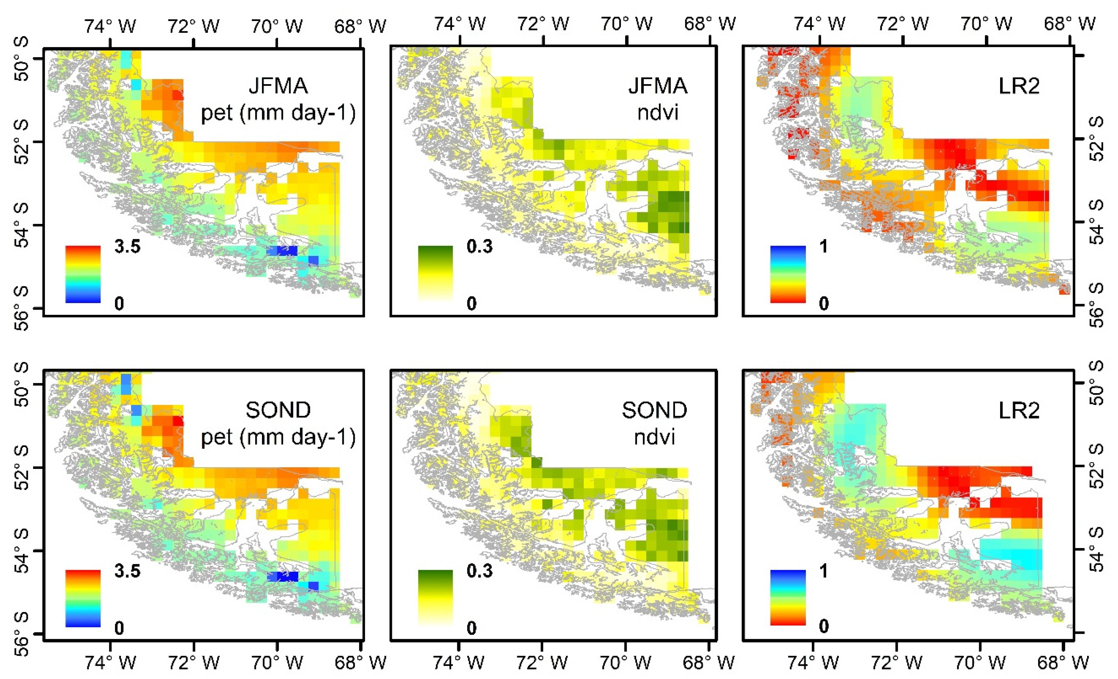
| NDVI (jfma) | pet (jfma) | Figure 5 | 0.67 | 0.62 | 39 |
| NDVI (sond) | pet (sond) | 0.77 | 0.74 | 57.5 | |
| NDVI (ann) | pre (ann) | Not shown | 0.73 | 0.63 | 30 |
| NDVI (ann) | tmn (ann) | Not shown | 0.66 | 0.59 | 25 |
| NDVI (ann) | pet (ann) | Not shown | 0.62 | 0.57 | 30 |
| Dependent Variables | Independent Variables | Reference | Correlation |
|---|---|---|---|
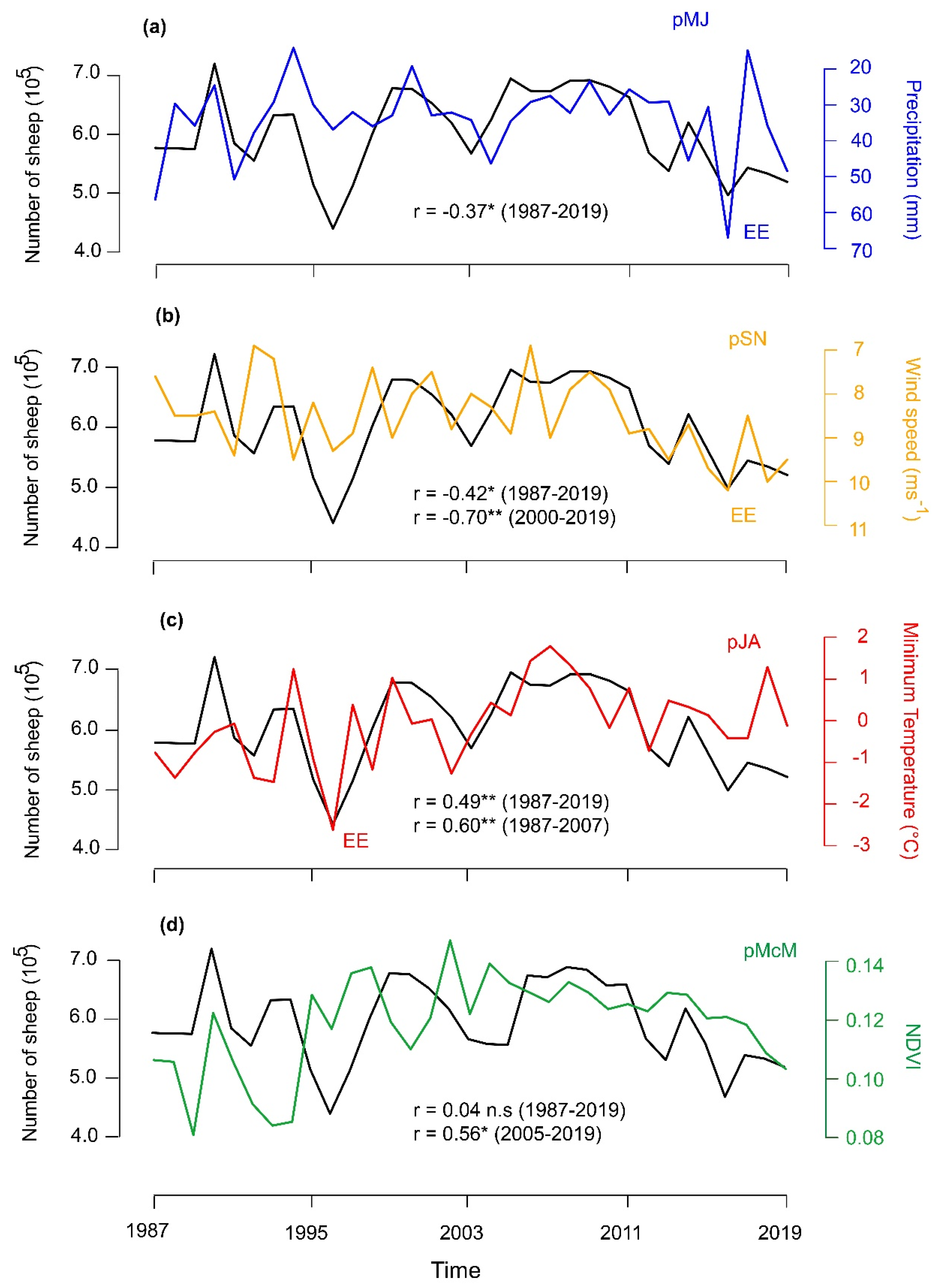
| SP | pre (MJ) | Figure 6a | −0.37 * (1987–2019) |
| SP | ws (SN) | Figure 6b | −0.42 * (1987–2019) −0.70 ** (2000–2019) |
| SP | tmn (JA) | Figure 6c | 0.49 ** (1987–2019) 0.60 ** (1987–2007) |
| SP | NDVI (pMcM) | Figure 6d | 0.04 n.s (1987–2019) 0.56 * (2005–2019) |
| SP | pre (ann) | Not shown | 0.24 n.s (1987–2019) |
| SP | ws (ann) | Not shown | −0.11 n.s (1987–2019) |
| SP | tmn (ann) | Not shown | 0.33 n.s (1987–2019) |
| SP | NDVI (ann) | Not shown | −0.14 n.s (1987–2019) |
© 2020 by the authors. Licensee MDPI, Basel, Switzerland. This article is an open access article distributed under the terms and conditions of the Creative Commons Attribution (CC BY) license (http://creativecommons.org/licenses/by/4.0/).
Share and Cite
Soto-Rogel, P.; Aravena, J.-C.; Meier, W.J.-H.; Gross, P.; Pérez, C.; González-Reyes, Á.; Griessinger, J. Impact of Extreme Weather Events on Aboveground Net Primary Productivity and Sheep Production in the Magellan Region, Southernmost Chilean Patagonia. Geosciences 2020, 10, 318. https://doi.org/10.3390/geosciences10080318
Soto-Rogel P, Aravena J-C, Meier WJ-H, Gross P, Pérez C, González-Reyes Á, Griessinger J. Impact of Extreme Weather Events on Aboveground Net Primary Productivity and Sheep Production in the Magellan Region, Southernmost Chilean Patagonia. Geosciences. 2020; 10(8):318. https://doi.org/10.3390/geosciences10080318
Chicago/Turabian StyleSoto-Rogel, Pamela, Juan-Carlos Aravena, Wolfgang Jens-Henrik Meier, Pamela Gross, Claudio Pérez, Álvaro González-Reyes, and Jussi Griessinger. 2020. "Impact of Extreme Weather Events on Aboveground Net Primary Productivity and Sheep Production in the Magellan Region, Southernmost Chilean Patagonia" Geosciences 10, no. 8: 318. https://doi.org/10.3390/geosciences10080318