Robust Force Control of Series Elastic Actuators

Department of Computer Science, University of Verona, Strada Le Grazie 15, Verona 37134, Italy
*
Author to whom correspondence should be addressed.
Actuators 2014, 3(3), 182-204; https://doi.org/10.3390/act3030182
Submission received: 16 December 2013
/
Revised: 16 May 2014
/
Accepted: 30 May 2014
/
Published: 9 July 2014
(This article belongs to the Special Issue Soft Actuators)
Abstract
:Force-controlled series elastic actuators (SEA) are widely used in novel human-robot interaction (HRI) applications, such as assistive and rehabilitation robotics. These systems are characterized by the presence of the “human in the loop”, so that control response and stability depend on uncertain human dynamics, including reflexes and voluntary forces. This paper proposes a force control approach that guarantees the stability and robustness of the coupled human-robot system, based on sliding-mode control (SMC), considering the human dynamics as a disturbance to reject. We propose a chattering free solution that employs simple task models to obtain high performance, comparable with second order solutions. Theoretical stability is proven within the sliding mode framework, and predictability is reached by avoiding the reaching phase by design. Furthermore, safety is introduced by a proper design of the sliding surface. The practical feasibility of the approach is shown using an SEA prototype coupled with a human impedance in severe stress tests. To show the quality of the approach, we report a comparison with state-of-the-art second order SMC, passivity-based control and adaptive control solutions.
1. Introduction
Several rehabilitation and assistive devices have been developed based on force-controlled elastic actuators [1,2,3]. Elastic actuators can provide a safe interaction with a human, while force control allows an active role of the patient, following the “assist as needed” paradigm to promote patient motor learning.
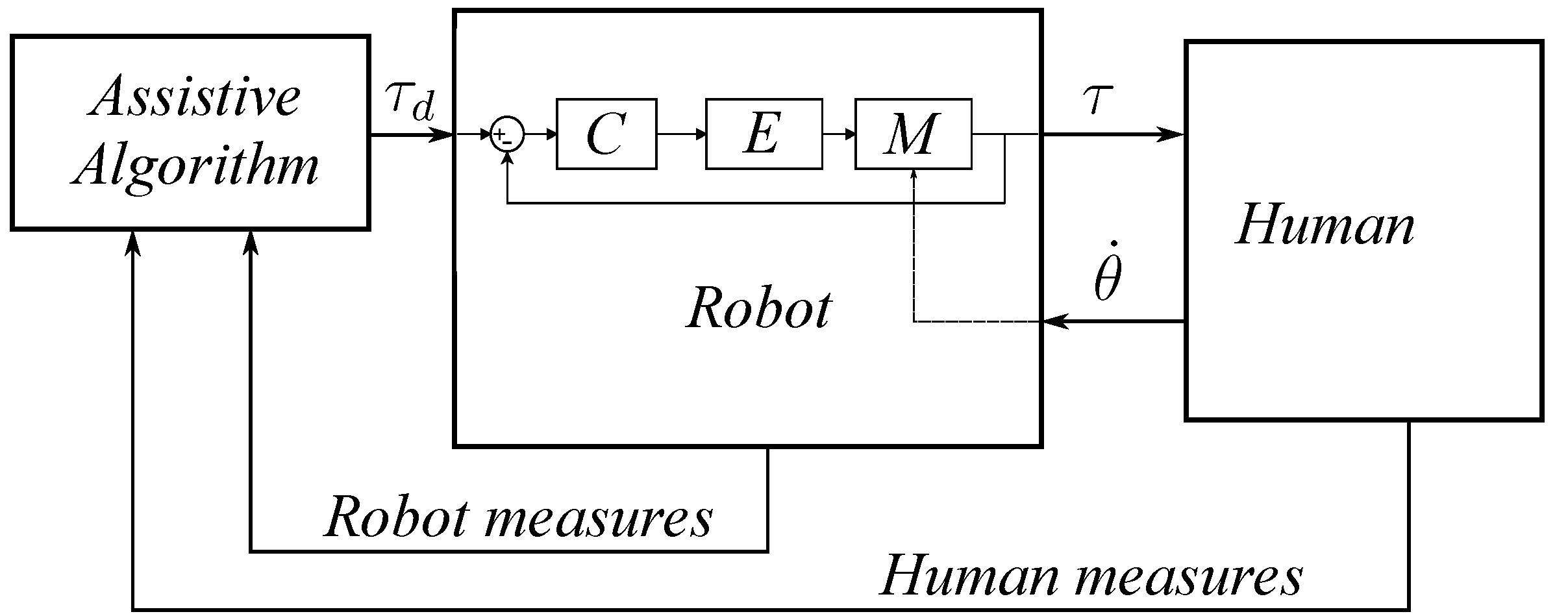
Force-controlled rehabilitation or assistive devices usually include two control layers. At the lower level, we have the force control layer that is usually strongly coupled to the human and requires fast computation and quick responses. At the higher level, we have a rehabilitation/assistive algorithm that computes the desired forces to be exerted. Examples of a rehabilitation/assistive algorithm are “path control” [4], “virtual model control” [5] or “CLIME” [6]. This two-layer architecture is represented in Figure 1, where the force control layer is embedded into the robot block. In this representation, causality is chosen, such as the force-controlled robot delivers forces to the human, who, in turn, exhibits a displacements. In this way, the robot acts as an impedance (having displacement as the input and force as the output) and the human as an admittance (having force as the input and position as the output), as suggested in [7].
Figure 1.
Typical rehabilitation robotics architecture based on force-controlled actuators. Symbols and M represent the force controller, the electronics and the robot mechanics, respectively. The interaction force/torque is represented by τ and the interaction velocity by .
Figure 1.
Typical rehabilitation robotics architecture based on force-controlled actuators. Symbols and M represent the force controller, the electronics and the robot mechanics, respectively. The interaction force/torque is represented by τ and the interaction velocity by .

In this work, we focus on stability and performance at the force control level, regardless of the specific assistive algorithm. Assuring the stability and well-defined performance of a “human in the loop system” is very challenging, because human modeling introduces many uncertainties, as already observed in the literature [8] and in our previous experience (In particular, in [9], one can observe the different force control responses when the orthosis is worn by the real patient instead of a manikin) [9,10]. Uncertainties can be addressed using classical robust control, which ensures the stability and desired performance within a well-defined uncertainty set, which is supposed to include the real system. This implies a demanding preparatory phase to design a nominal model and to quantify uncertainties. An example of this approach can be found in [11], where the author considers a non-linear musculo-skeletal model with parametric uncertainties. Another example is [12,13], where a simpler human model is assumed and an automatic procedure is proposed to search for an optimal stable controller.
A simpler and widely-used alternative is based on passivity theory. In fact, it is known that the feedback connection of two passive systems is still passive and, thus, stable. Hence, it is possible to guarantee stability by simply assuring the passivity of the controller, assuming that the human-robot system can be considered passive [14,15]. This strategy is very attractive, because it does not need the knowledge of the human model nor to deal with uncertainties. However, there is a main drawback, due to the fact that a passivity-based controller needs to be stable against all kinds of external passive environments; no matter what kind of environment and no matter its scale (i.e., its level of inertia, stiffness, damping, etc.). It follows that this approach neglects almost all environmental dynamics; therefore, it is not possible to speculate on control performance, in the traditional sense of the term. We mean that the dynamics of the controlled quantity, i.e., the force, cannot be defined. In fact the authors that propose passive controllers for HRI usually define impedance dynamics, which actually is not the force dynamics [16,17].
To summarize current research, we can say that the way the human dynamics is considered leads to different interaction control approaches. In classical robust control, the human is represented as a model set, which can be difficult to characterize and can involve complex design. In existing passivity-based approaches, the human is simply considered as a passive system. Control design results are highly simplified, but it is not possible to guarantee any control performance. Finally, in the adaptive approach proposed in [18], the human is regarded as a second order system, whose parameters are on-line estimated, providing well-defined performance, but only when the system is coupled to a second order environment.
A fourth approach to HRI can be based on implicit impedance control, as proposed in [7], where open loop force control is used to shape the impedance of the robot. However, this solution is not suitable if we employ elastic actuators. This is because we do not simply need to deliver a force, but also to control the dynamics of the elastic element. For this reason, the impedance control of elastic actuators always includes an explicit force loop [19,20] whose performance is influenced by human dynamics.
A fifth approach exists in the literature, which does not make any assumption on the environment and simply considers it as a disturbance to reject. In [8], the authors propose a torque controller that uses a disturbance observer within an inner motor position loop. In [21], a more intuitive control architecture is proposed, based on a similar principle. However, it is not clear why the authors estimate the motor position, whereas it is measured. The disturbance observer approach has been judged as “difficulty in the design” and with “unexpected instability” in [22] (by the same authors of [8]); then, a basic sliding mode controller has been proposed, but just to compensate for uncertain actuator parameters (instead for unknown human dynamics). Quite unexpectedly, in all of these works, the disturbance is identified with human position, which is actually measurable.
In this paper, the disturbance is identified with only the unmeasured part of the human dynamics, i.e., human position derivatives; thus, we better account for the interaction nature of the problem (involving both the actuator and human dynamics). Then, we ensure stability and performance by designing a controller that is insensitive to such a disturbance. We propose an approach based on advanced sliding-mode algorithms that are proven to attract the state towards a stable, well-defined region in the state space, which defines the force dynamics in spite of uncertainties [23,24]. We show that by a proper design of the SMC law, it is possible to guarantee well-defined and deterministic (i.e., not influenced by the environment) force control performance. We also propose an improvement of the linear SMC approximation that is based on a simple task model, i.e., a periodic task, to improve control accuracy. We show the practical feasibility of the proposed algorithm in an experimental setup where an SEA is coupled with a human arm.
2. Sliding-Mode Control
In this section, we briefly summarize the classical SMC concepts and derived algorithms. SMC is a non-linear control method characterized by high simplicity and robustness. It has been shown that certain SMC algorithms can handle the position control problem with high safety. For this reason, such algorithms have been already applied to position controlled assistive and rehabilitative devices [25,26,27,28]. We show in the following that to retain the same kind of safety in the force control problem, we need to apply a particular sliding-mode design. Furthermore we observe that certain sliding-mode variants that focus on safety, such as the proxy-based SMC [29], lose the theoretical robustness guaranteed by the SMC framework. For this reason, these algorithms are not discussed in this work.
2.1. Sliding-Mode Concepts
SMC can be applied to the tracking control of the generic n-th order system in the companion form:
where f is a non-linear map, assumed known, is the state vector, u is the system input and υ is an additive bounded disturbance, such as , where V is a positive known function or constant. Sliding-mode controllers utilize a discontinuous control law to drive the system state onto a sliding surface in the state space in finite time (reaching phase) and to keep the system state on this manifold for all the subsequent times (sliding mode or sliding regime). The advantages of this approach are that the dynamics of the system while in the sliding regime is of reduced order, and it is insensitive to a common class of model uncertainties or disturbances, called matched noise [30]. This implies robust control performances when in the sliding regime, where desired performance is specified by sliding surface design. In spite of the claimed robustness properties, the practical implementation of SMC presents a major drawback, called the chattering effect. It consists of a residual high frequency vibration that occurs because of the discontinuous nature of the control law, combined with the limited switching frequency of real-world instrumentation. A sliding surface can be defined using the following notation:
where is the tracking error and λ is a positive design parameter that determines the control convergence rate, i.e., the control performance in the sliding regime. Note that control performance can be defined only in the sliding regime and not during the reaching phase. Taking as an example Equation (1) in the case of second order system (), we can define the sliding surface:
If we neglect the disturbance, , the effort to slide on the sliding surface can be computed as:
which can be considered the best approximation of the equivalent control, that is an ideal continuous control able to keep the state on the sliding surface, exactly compensating for uncertainties. Note that by applying the ideal equivalent control, we have ; instead, by applying its approximation, , we have . The SMC solution dominates the disturbance, , by adding a large discontinuous term:
where and ϵ is an arbitrary small positive constant. It can be shown that this control law satisfies the reaching condition [24]:
Thus, it drives the system to the sliding surface in finite time, despite uncertainties in . It must be noted that the parameter, , in Equation (5) is usually chosen as constant, so that the discontinuous term is bounded. On the other hand, the equivalent control approximation, , can be unbounded, depending on the system dynamics. It should be highlighted that the design of equivalent control approximation is an important step of sliding-mode design, because everything we discard in the approximation must be bounded and will be handled by the discontinuous term. In particular, the wider the uncertainty bound is, the larger the chattering amplitude will be.
2.2. Continuous Approximation of SMC
The continuous approximation solution is the easiest way to reduce/eliminate the chattering effect. It consists of substituting the discontinuous part, , in Equation (5) by a continuous approximation. Common examples use a sigmoid or a linear approximation, such as the function, , defined as:
It can be proven that, using such an approximation in place of the discontinuous term in Equation (5), the system state reaches the boundary, , in a finite time and subsequently remains inside of it; thus, stability is achieved in the sense of boundedness. The choice of Φ represents the thickness of the boundary layer. For , the boundary collapses on the sliding surface, and we have standard SMC with high robustness and chattering; on the other hand, increasing Φ the control response becomes smoother, but also more sensitive to disturbance (in fact, inside the boundary, the system trajectories are unpredictable).
2.3. Higher Order SMC
Higher order sliding-modes are an extension of the SMC concept, which attempt to reduce the chattering effect, while retaining the theoretical exact tracking. In particular, second order sliding-modes represent the widest used class of higher order SMC, because they are quite simple to implement. In fact, they only need the measure of w and, only in some cases, of . In general, it can be said that the higher the order is, the more measurements that are required, in terms of state derivatives.
In a second order SMC, the discontinuity acts on instead of on w. The switching logic can be based both on w and and should guarantee the finite time convergence to the sliding surface, defined as . Three main second order algorithms are proposed in the literature: the twisting, the sub-optimal and the super-twisting, in historical order. The reader can refer to [31,32] for details. These algorithms are usually superior to first order solutions, but are less intuitive to tune and may use an integral action that reduces safety, as explained in Appendix A.
3. Compliant Interaction Model
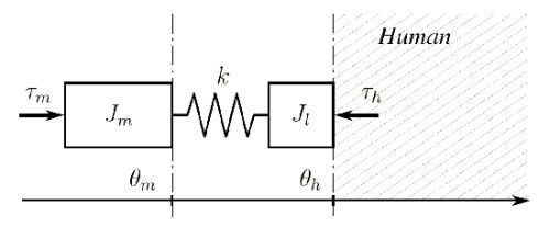
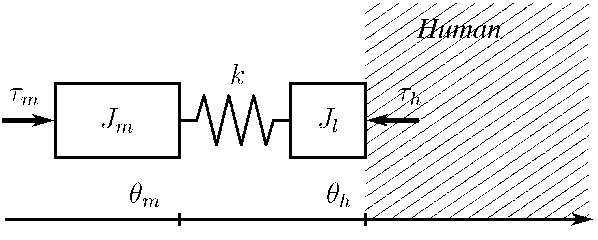
The interaction between an SEA and a human of unknown dynamics is represented in Figure 2, where for the simplicity of representation, angular quantities have been converted into linear equivalents. A torsional spring of stiffness k is arranged between a motor of inertia and a link of inertia , which is in contact with the human. In Figure 2, the variable, , is the motor input torque, is the motor position, is the human joint position, is the torque exerted by the spring (pointing toward the human) and is the torque exerted by the human. The relations among these variables can be written as:
The motor is supposed to be driven by a current loop with negligible dynamics, and the link is considered lightweight, i.e., with negligible inertia w.r.t. the coupled human inertia. Such a design allows one to control the interaction by controlling . Angular positions and velocities are considered measurable, while accelerations are not.
Figure 2.
Representation of a human-robot interaction using a series elastic actuator (SEA). The human dynamics is considered unknown, and it is represented as the dashed area.
Figure 2.
Representation of a human-robot interaction using a series elastic actuator (SEA). The human dynamics is considered unknown, and it is represented as the dashed area.
The system to be controlled needs to be expressed with as the input and as the output and can be derived from Equation (8) as:
where represents the system input and the unknown human joint torque, retained as a disturbance.
4. System Control
In this section, we describe the control design step and explain the advantages of integral SMC w.r.t. standard SMC in the considered control problem. Integral SMC has the main advantage of avoiding the reaching phase, which is highly undesirable, because during this transient, the system is subject to unpredictable dynamics. Furthermore, we will show that with integral SMC, it is possible to avoid feedback inversion in the equivalent control approximation, which can be harmful, especially in the case of approximated implementations, as in Equation (7).
Section 4.1 analyzes the disturbance introduced by the human. Section 4.2 describes the design of equivalent control approximation, and Section 4.3 proposes a candidate SMC approximation based on periodic task models.
4.1. Disturbance Analysis
Uncertainties are represented in Equation (9) by the human joint torque, , whose magnitude can be very high. Note that System (9) can be rewritten in a more convenient form:
where have been replaced with , according to Equation (8). Now, uncertainties are represented by the human joint acceleration, , which depends on the human dynamics, including mechanical impedance, neural mechanisms and motor control. In practical applications, can be estimated with a filtered finite difference approximation, , introducing an additive system uncertainty represented by . Thus, we can rewrite Equation (10) as:
The finite difference approximation is known to introduce uncertainties in the high spectrum. Moreover, if the velocity measure is derived from position sensors, the noise, , can be high in the case of slow motion, because of position quantization.
4.2. Control Design
An interesting aspect of integral SMC is that, by a proper initialization of the integral term, it is possible to avoid the reaching phase, having the state on the sliding surface from the beginning. This allows one to assure predictable control performance. In fact, the duration of the reaching phase is finite, but, in general, unknown, as it depends on uncertain dynamics. By avoiding the reaching phase, we ensure that desired control specifications are always fulfilled. To this aim, the integral error should be reinitialized whenever the state exits from a sliding surface neighborhood, as we will detail.
In the following, we start from the standard SMC design to then show the advantages of integral SMC. If we define the standard sliding surface:
where and λ is a positive design parameter, we can compute the equivalent control approximation from Equation (11) by setting and neglecting the uncertain term . It results:
that, by replacing , it can be rewritten as:
where the first two terms on the right-hand side can be interpreted as a proportional-derivative action with and . Unfortunately, it is not usually a good choice to have negative proportional gain (i.e., positive proportional feedback) if high robustness is desired. As a demonstration, we can consider an example where the human is modeled as a pure inertia, :
In this case, the system to control can be expresses as:
Then, if we consider a generic proportional-derivative controller , we find the following closed loop transfer function:
that is stable for and . If now, we put in the case of the control Law (14) with , the resulting gain margin is , which can be inadequate if the motor inertia is small with respect to the human inertia.
Even if in SMC theory there are no robustness requirements on the equivalent control approximation, as robustness is achieved through the discontinuous term in Equation (5), in practice, a well-behaving equivalent control approximation is desirable, especially in the case that we use a continuous approximation. In the following, we show that the integral SMC not only ensures predictable performances, but can also augment the robustness of equivalent control approximation, by avoiding positive feedback.
Let us consider the following integral sliding surface:
where and are positive design parameters and is the error integral over the interval , where is the starting time and t is the current time. By considering and substituting the system dynamics (11), it is possible to compute the equivalent control approximation:
where and . It follows that parameter defines the gain margin of equivalent control (19), as previously discussed. Interestingly, if , it is possible to avoid feedback inversion having positive and . As a particular case when , the proportional gain disappears, and the control effort is bounded even in the case of indefinitely high errors. This leads to improved safety, as detailed in Appendix A.
Parameters and also define the control performance when in the sliding regime, as reported in Section 2. Unfortunately, such robust control performance cannot be met during the reaching phase, which should be avoided by design. For this reason, it is necessary to reinitialize the integral term in Equation (18) as the state goes far from the sliding surface. In particular, we simply need to pose:
whenever is greater than a certain acceptable threshold, . In this way, the error dynamics is defined by . This means that we avoid the reaching phase, even in the cases of system initializations, failures or discontinuous references.
4.3. Improving the Accuracy within the Boundary
A solution to reduce the chattering is to substitute the discontinuity in Equation (5) with the continuous linear approximation (7). In this case, the system state converges to the boundary, , where it moves unpredictably. In this sliding-boundary regime, the applied control is de facto a high-gain linear control, whose structure depends on the sliding surface design. Here, accuracy can be enhanced by the internal model principle [33]. In particular, if we consider periodic tasks, they can be easily described in the frequency domain. Examples of such tasks are locomotion activities, such as walking, running, trotting or swimming. To provide the internal model for a periodic force task, we propose to introduce a resonator in the control law having the same base frequency of the task. The proposed controller is implemented by substituting the function, , in Equation (5) with , defined, using mixed time-frequency notation, as:
where s is the Laplace variable and is a gain that multiplies the resonator, , of frequency and damping ψ:
Outside the boundary, the continuous approximation is left unmodified, so the finite time convergence to the boundary is retained. When inside the boundary, we can imagine two additive control efforts. On one side, the equivalent control approximation leads the system to behave like:
where is generically intended as residual disturbance, neglected by equivalent control approximation. On the other side, the effect of the proposed function, , brings the system dynamics to be:
using mixed time-frequency notation. Consequently the dynamics of w can be seen as a random process, where the noise, , feeds the third-order transfer function:
where the denominator coefficients are . The effect of Filter (25) is double: at the denominator, we have a low pass-filter, while at the numerator, we have a notch filter, which can significantly reduce the disturbance in the vicinity of . Note that the tuning of is to be considered task specific; thus, it is valid independently of the particular system or environment.
We highlight that the key concept of the presented analysis is the interpretation of Equation (23) as a linear transfer function having as an exogenous input. We highlight also that boundedness (i.e., convergence to a boundary) is a typical phenomenon of real-world SMC implementations, and in general, the wider the boundary is, the less the chattering will be. In this light, we think that the general idea of using linear tools within such a boundary can be very helpful in practice, because it retains the simplicity and effectiveness of the linear filter design.
5. Experimental Results
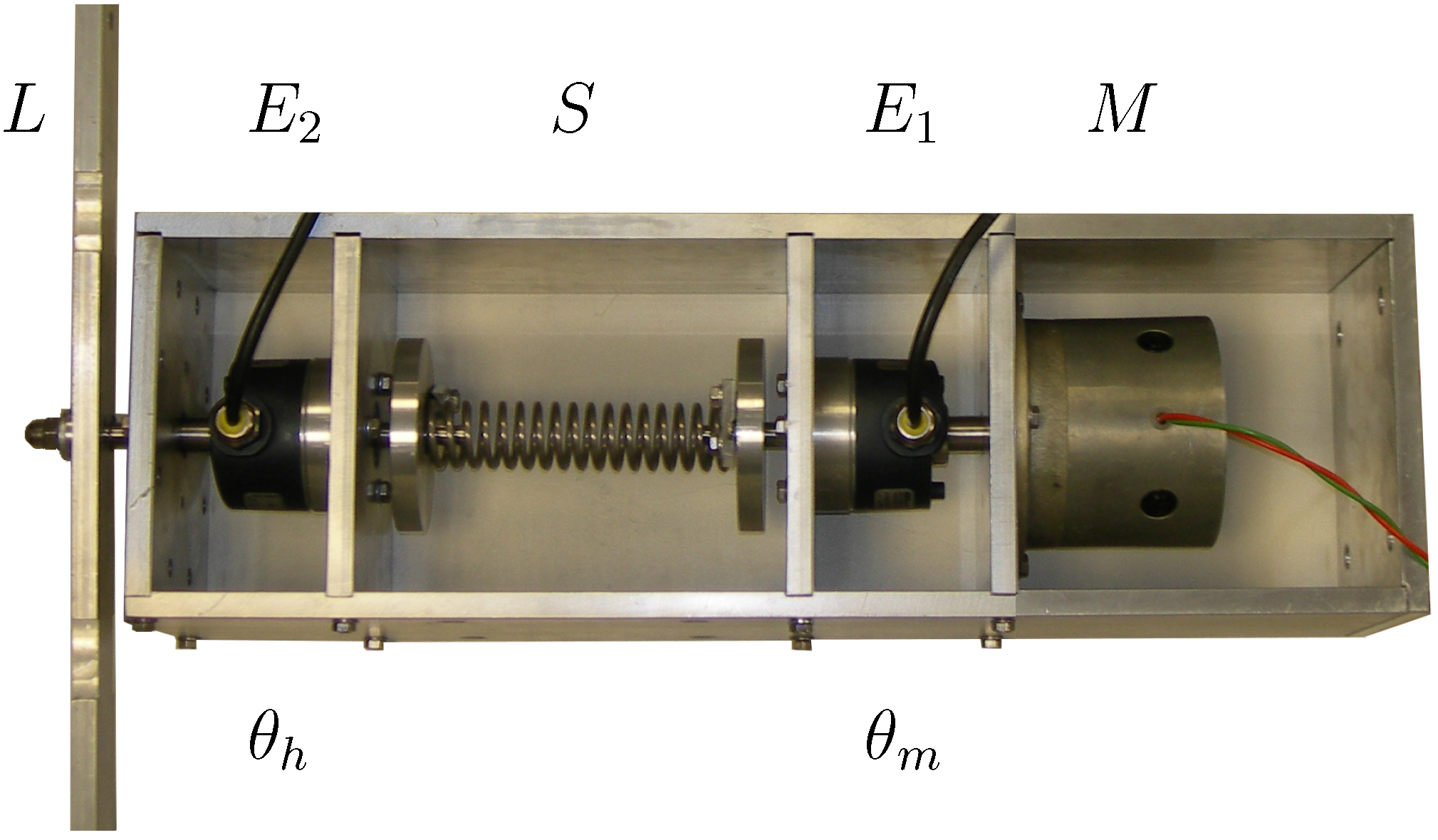
We implemented the described algorithms to control the SEA prototype in Figure 3, composed of a torque motor connected in series to a spring and then to an arm support. Two high accuracy encoders are used to measure motor position and spring displacement with a resolution of degrees. Velocities are obtained by measuring pulse inter-periods, using hardware interrupts. This gives a better approximation with respect to finite differences, especially in the case of higher velocities, where several inter-periods are averaged. The system parameters have been estimated using a procedure similar to that described in [34] and are reported in Table 1.
Figure 3.
The SEA prototype used as the testbed. The motor, M, is connected to the spring, S, and the angular quantities, and , are measured by encoders and , respectively. L is the arm support that is a pure inertial load when the system is not interacting with the human.
Figure 3.
The SEA prototype used as the testbed. The motor, M, is connected to the spring, S, and the angular quantities, and , are measured by encoders and , respectively. L is the arm support that is a pure inertial load when the system is not interacting with the human.


| Parameter | Symbol | Value |
|---|---|---|
| Spring Stiffness | k | 1.040 Nm/rad |
| Torque constant | 0.42 Nm/A | |
| Motor inertia | 0.00041 kg/m | |
| Wood load inertia | 0.00025 kg/m | |
| Metal load inertia | 0.00390 kg/m |
The control system runs on a standard PC equipped with a quad-core processor and a real-time Linux kernel. Real-time is obtained using a process with kernel-like priority and a system sleep function with the granularity of some nanoseconds (nanosleep). The control process runs at 3 kHz and communicates with the motor drive and the sensor electronics via the Ethercat protocol at the same rate.
Five sliding-mode controllers are implemented as shown in Table 2, where relative acronyms are reported. The first is a basic first order sliding-mode algorithm (SM); the second considers an integral sliding surface (ISM); the third is a linear approximation of the second (ILA); and the fourth introduces the proposed internal model rejection by adding a resonator (ILAR). Finally, we considered also a super twisting algorithm (STW), which has been reported to be experimentally superior w.r.t. other second order SMCs [35].
| Control Law | Acron. | Sliding Surface | k | |
|---|---|---|---|---|
| SM | standard (3) | (14) | ||
| ISM | integral (18) | (19) | ||
| ILA | integral (18) | (19) | ||
| ILAR | integral (18) | (19) | ||
| Super Twisting | STW | integral (18) | (19) | * |
The value indicates the amplitude of the term with the discontinuous derivative. Note that this is not the unique parameter to tune in the STW algorithm.
The gain, k, is tuned by trial and error to obtain a sliding regime. Parameters and are set to and , respectively, for all of the controllers to have critically damped control dynamics and a bounded control effort, as explained in Appendix A. The resulting control bandwidth when in the sliding regime is 8 Hz. The linear approximation boundary is set to ; the resonator frequency is set to 4 Hz, and its damping is set to slightly <1. In the case of integral sliding-mode, we implemented the integrator re-initialization, as explained in Section 4.2, using the threshold .
5.1. Qualitative Analysis
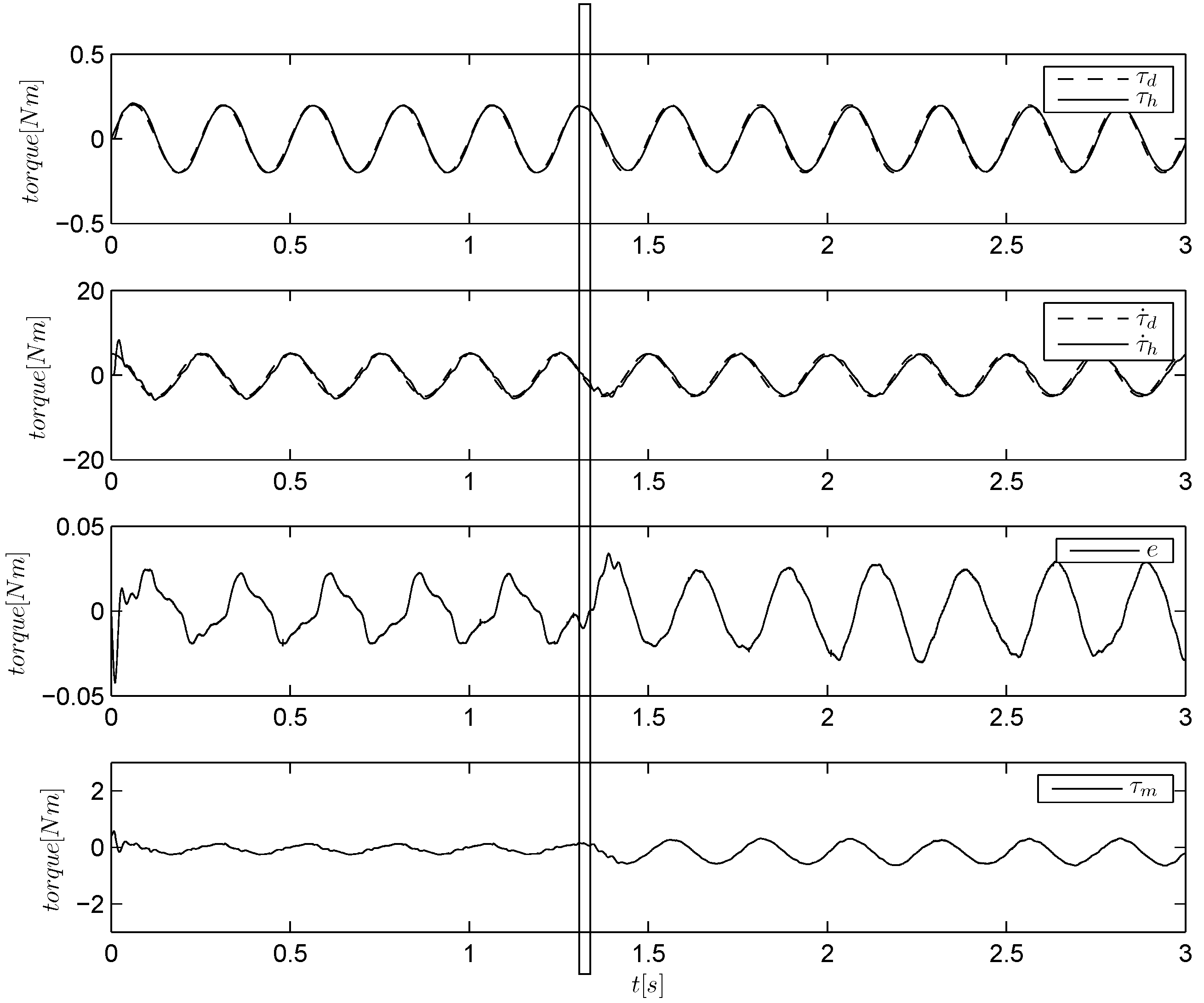
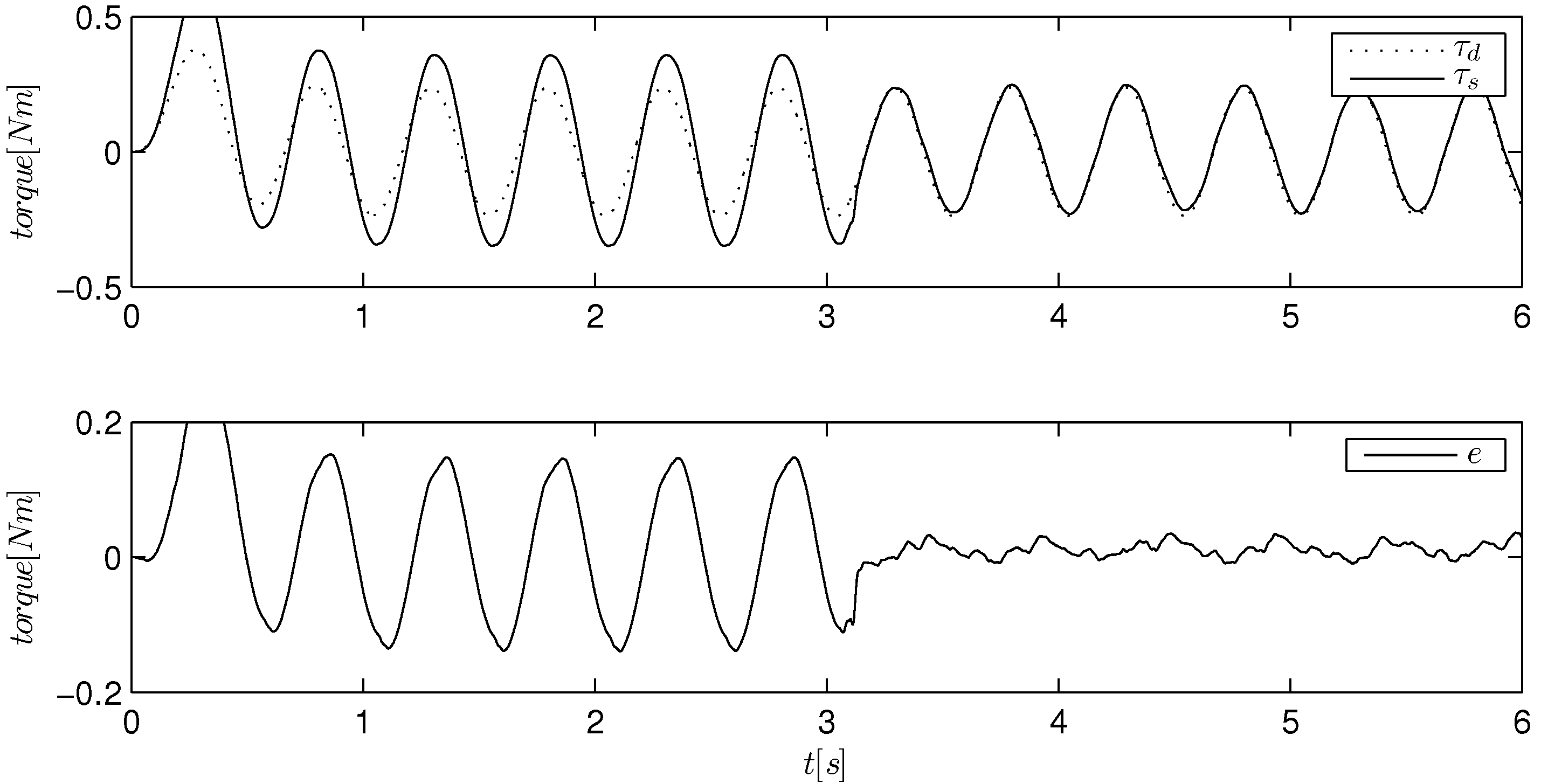
Experiments are designed to test control robustness in the worst case conditions, that is when the human dynamics is subject to high uncertainty and sudden variations. To this aim, we replaced the metal support L in Figure 3 with a wood frame. In fact, as the wood fame is very lightweight, the magnitude of the uncertain term, the acceleration, , can become very high. Furthermore we created a high impedance condition by holding the wood frame by hand and trying to be as stiff as possible. Figure 4, Figure 5, Figure 6, Figure 7, Figure 8 and Figure 9 show the responses of the different controllers during torque tracking experiments, where we keep the high impedance for a few initial seconds, and then, we release the frame, reaching an extremely low impedance condition. The torque reference is a 4-Hz sinusoid of an amplitude of 0.2 Nm. For each algorithm, we plot the torque signal, its derivative, the torque error and the control input, . We indicated with a vertical bar the impedance change. Note that immediately after this change, the control input varies its amplitude to retain the same tracking performance. The plot of SM algorithm is not reported, as it behaves similarly to ISM algorithm (Figure 5); a more significant comparison between SM and ISM is reported in the following.
By observation of Figure 4, Figure 5, Figure 6, Figure 7, Figure 8 and Figure 9, one can see that the torque tracking is always retained in both high and low impedance conditions with reasonable levels of accuracy, but different levels of chattering. In particular, both the ILA and ILAR algorithms (Figure 6 and Figure 8) show a chattering-free response, while the STW algorithm (Figure 9) exhibits some chattering if tuned to meet the required robustness.
Figure 4.
Torque tracking of a sinusoidal reference with the SM algorithm. The load is held by hand and then released at about s.
Figure 4.
Torque tracking of a sinusoidal reference with the SM algorithm. The load is held by hand and then released at about s.
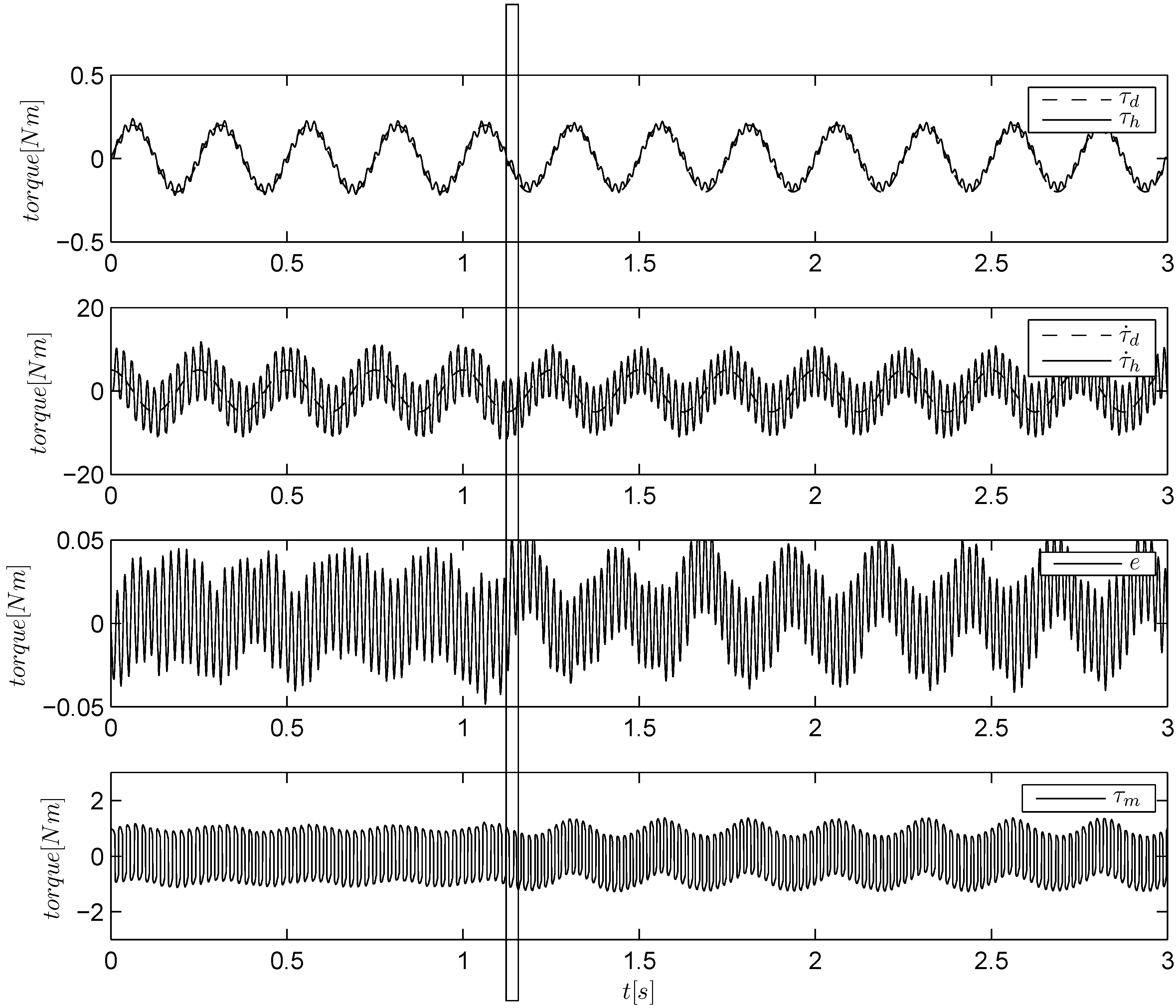
Figure 5.
Torque tracking of a sinusoidal reference with integral sliding-mode (ISM algorithm). The load is held by hand and then released at about s.
Figure 5.
Torque tracking of a sinusoidal reference with integral sliding-mode (ISM algorithm). The load is held by hand and then released at about s.

Figure 6.
Torque tracking of a sinusoidal reference using a linear approximation (ILA algorithm). The load is held by hand and then released at about s.
Figure 6.
Torque tracking of a sinusoidal reference using a linear approximation (ILA algorithm). The load is held by hand and then released at about s.

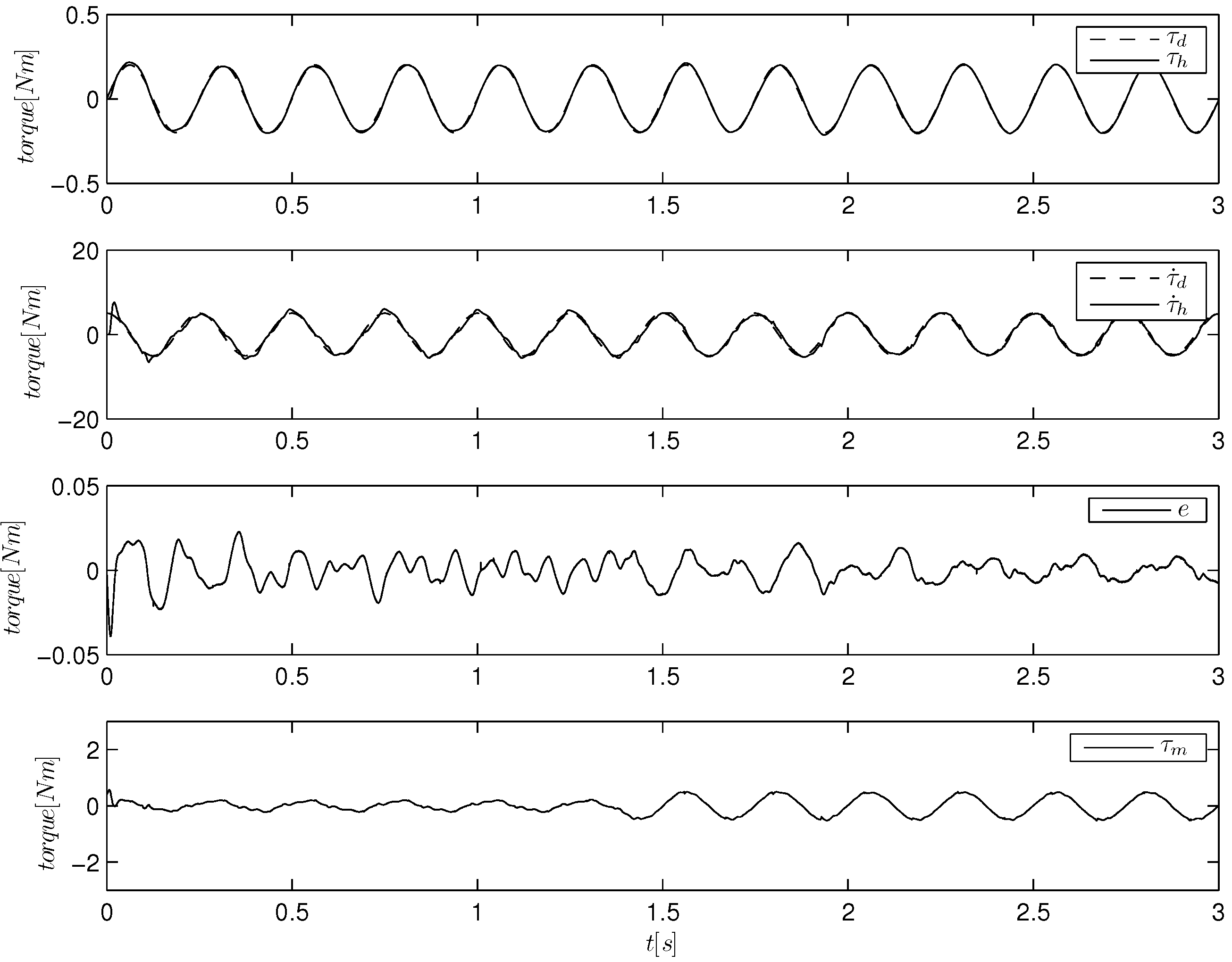
Figure 7.
Torque tracking of a sinusoidal reference using a linear approximation and a periodic task model (ILAR algorithm). The load is held by hand and then released at about s.
Figure 7.
Torque tracking of a sinusoidal reference using a linear approximation and a periodic task model (ILAR algorithm). The load is held by hand and then released at about s.

Figure 8.
Torque tracking of a sinusoidal reference using the ILAR algorithm in a longer experiment to better see the resonator dynamics (sometimes, it is necessary for the resonator to acquire the oscillating energy). The load is held by hand and then released at about s.
Figure 8.
Torque tracking of a sinusoidal reference using the ILAR algorithm in a longer experiment to better see the resonator dynamics (sometimes, it is necessary for the resonator to acquire the oscillating energy). The load is held by hand and then released at about s.
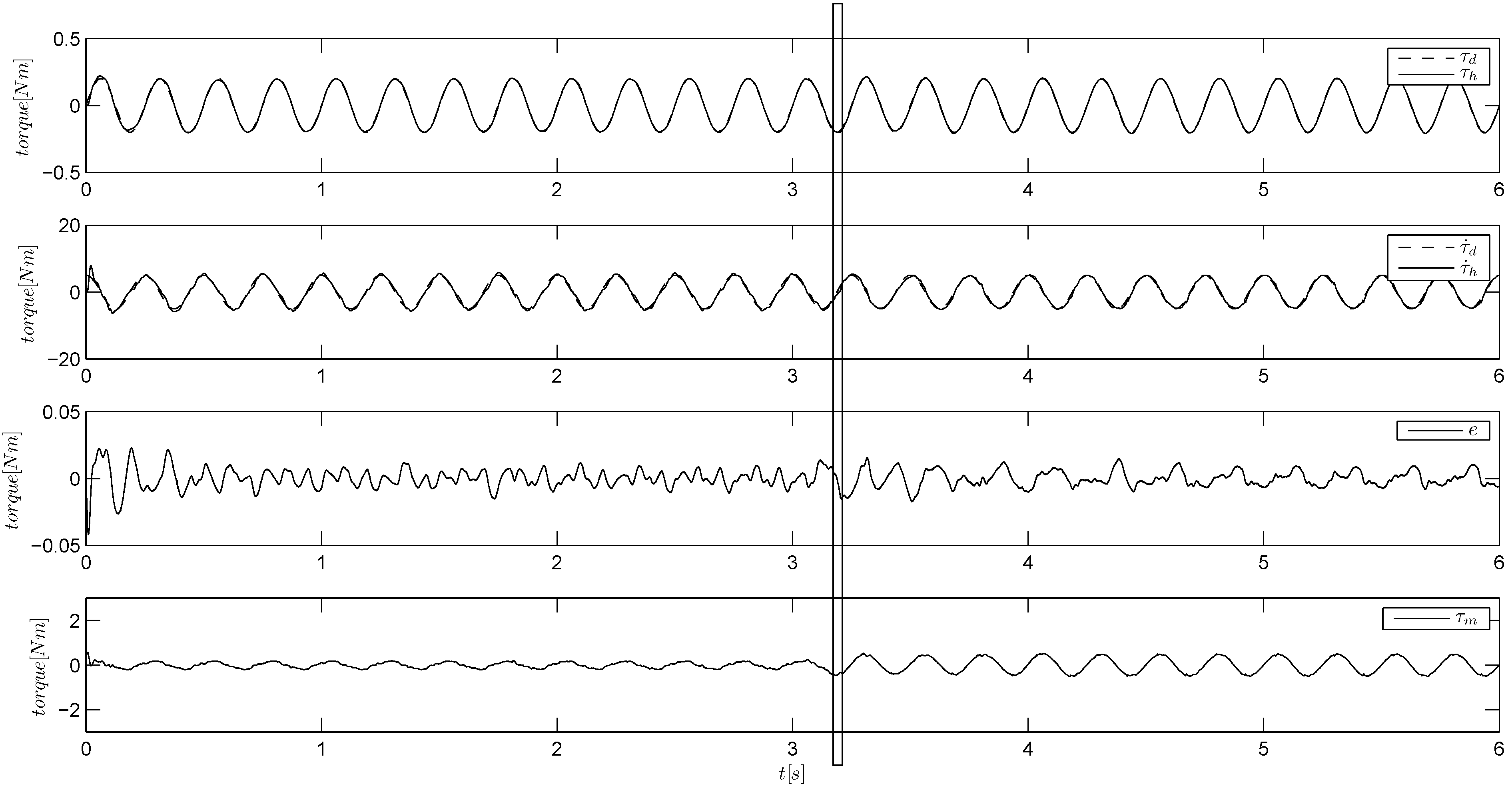
Figure 9.
Torque tracking of a sinusoidal reference using the STW algorithm. The load is held by hand and then released at about s.
Figure 9.
Torque tracking of a sinusoidal reference using the STW algorithm. The load is held by hand and then released at about s.
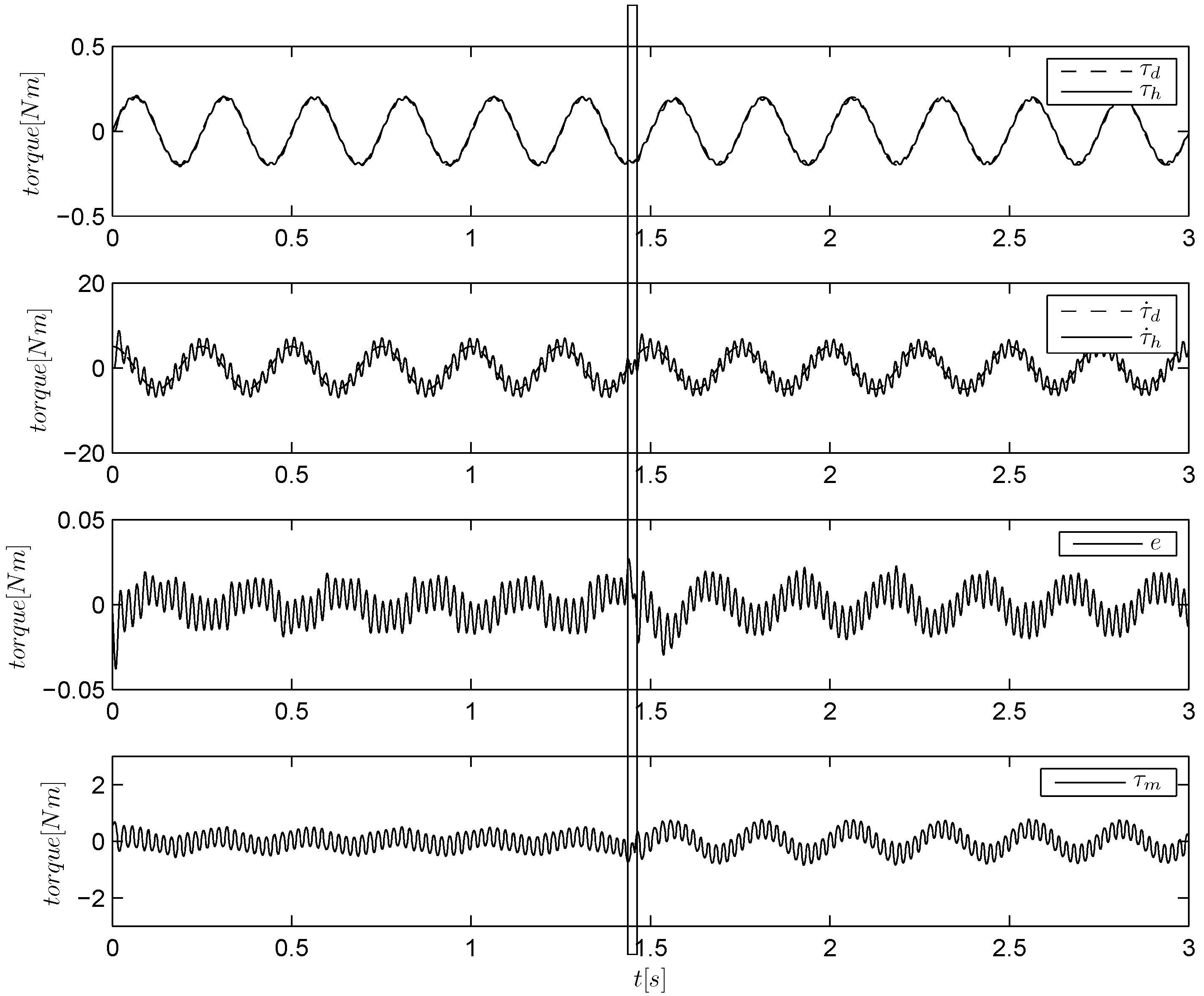
Figure 10 shows a step comparison between standard and integral sliding-modes in a high impedance condition. One can notice that the ISM and ILA algorithms provide the same kind of responses for different step amplitudes. This is because integral SMC with initialization (20) provides fully predictable (i.e., robust) control performance. On the other hand, the SM algorithm presents a non-exponential reaching phase, the duration of which depends on the step amplitude. This can be easily seen by comparing the left- and right-side plots, where in the latter case, the reaching time nearly doubled. We also highlight that in SMC theory, the reaching phase is sensitive to disturbance, so that the reaching time cannot be a priori known. Only when in the sliding regime, we have the SMC claimed robustness.
Finally, we observed that if we set the gain , we have that the SM algorithm is unstable, while the ISM algorithm is till stable. The observed instability is due to the weak stability margins of equivalent control (14), as explained in Section 4.2.
To provide a comparison between the proposed SMC approach and existing solutions, we show the behavior of a couple of passive controllers and an adaptive controller. The passive PID controller proposed in [36] is tuned with , and with a 1-Hz roll-off frequency (according to passivity constraints). Its response is shown in Figure 11. Errors are quite low in the high impedance case, but they increase when the load is released. Note that the error scale is magnified with respect to previous figures. To have a good performance in the low impedance condition, we use a passive PD controller computed with the pole placement method, by explicitly considering the wood inertia as the load in the system model. By considering 15-Hz critically damped poles as the reference, we found and , whose positiveness ensures the passivity of the controller [36]. Figure 12 shows that the response is accurate in the low impedance case, but it has significant overshoots when the impedance is high. The comparison with the proposed SMC approach is immediate: the passive controllers show a stable behavior as expected, but they cannot provide the same kind of force dynamics in different environments.
Figure 10.
Step response comparison among the SM (top), ISM (middle) and ILA (bottom) algorithms. The left and right figures show the responses to a step of an amplitude of 0.5 and 1.0 Nm, respectively. Note that the reaching time of the SM algorithm is about 0.1 s on the left plot and 0.2 s on the right plot.
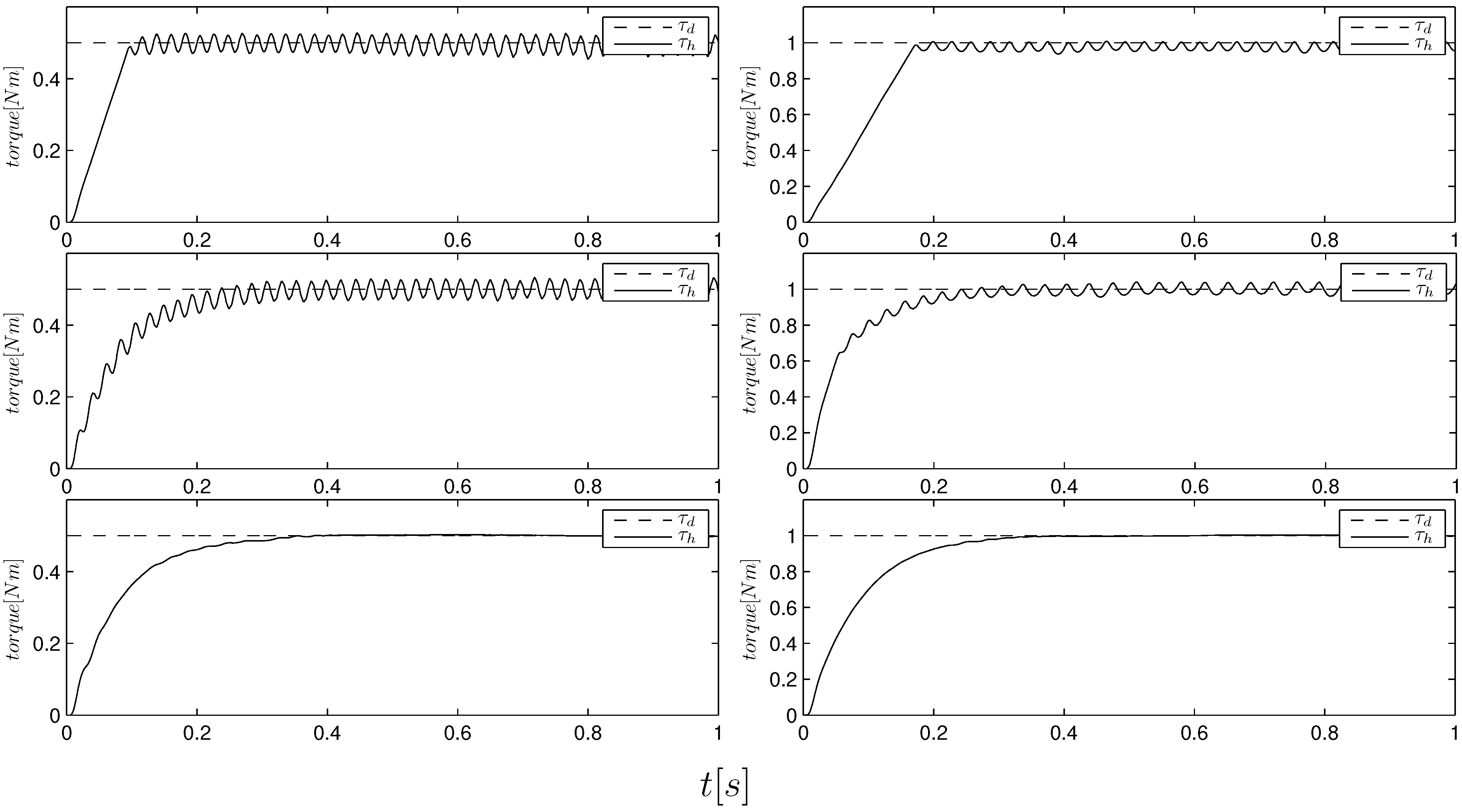
Figure 11.
Torque tracking of a sinusoidal reference using a passive PID. The load is firstly held by hand and then released at about s. Note that the error scale is zoomed out with respect to the previous figures.
Figure 11.
Torque tracking of a sinusoidal reference using a passive PID. The load is firstly held by hand and then released at about s. Note that the error scale is zoomed out with respect to the previous figures.

Figure 12.
Torque tracking of a sinusoidal reference using a passive PD controller tuned on a free load condition. The load is firstly held by hand and then released at about s.
Figure 12.
Torque tracking of a sinusoidal reference using a passive PD controller tuned on a free load condition. The load is firstly held by hand and then released at about s.
5.2. Quantitative Analysis and Comparison
In the following, we propose a comparison between the chattering-free SMC algorithms (ILA and ILAR) and the adaptive controller (AD) we proposed in [18], using in the latter case an 8-Hz critically damped reference model. Some details about the controller are reported in Appendix B, and a quantitative comparison w.r.t. passive algorithms is reported in [18], showing highly improved accuracy (up to ten times). The main advantage of SMC w.r.t. adaptive control is that stability is guaranteed against any kind of environmental coupling. In fact the adaptive approach is proven to be stable only when coupled to second order impedances. Furthermore, if the environment suddenly changes, it needs a little time to adapt. In Table 3, we report a comparison of the main theoretical and practical difference between the adaptive and sliding-mode approaches.
| Adaptive | Sliding-Mode (ILA/ILAR) | |
|---|---|---|
| Stability | In the sense of boundedness | In the sense of boundedness (sliding boundary) |
| Assumption for stability | Bounded human forces, second order human model | Bounded human accelerations |
| Human model | Second order linear system | Any |
| Accuracy | High accuracy is observed | A frequency model of the task is needed for high accuracy |
| Sensors | Environment position not required (force sensor) | Environment position (or velocity) required |
| Tuning | No tuning is necessary | Disturbance bound, boundary layer and task frequency |
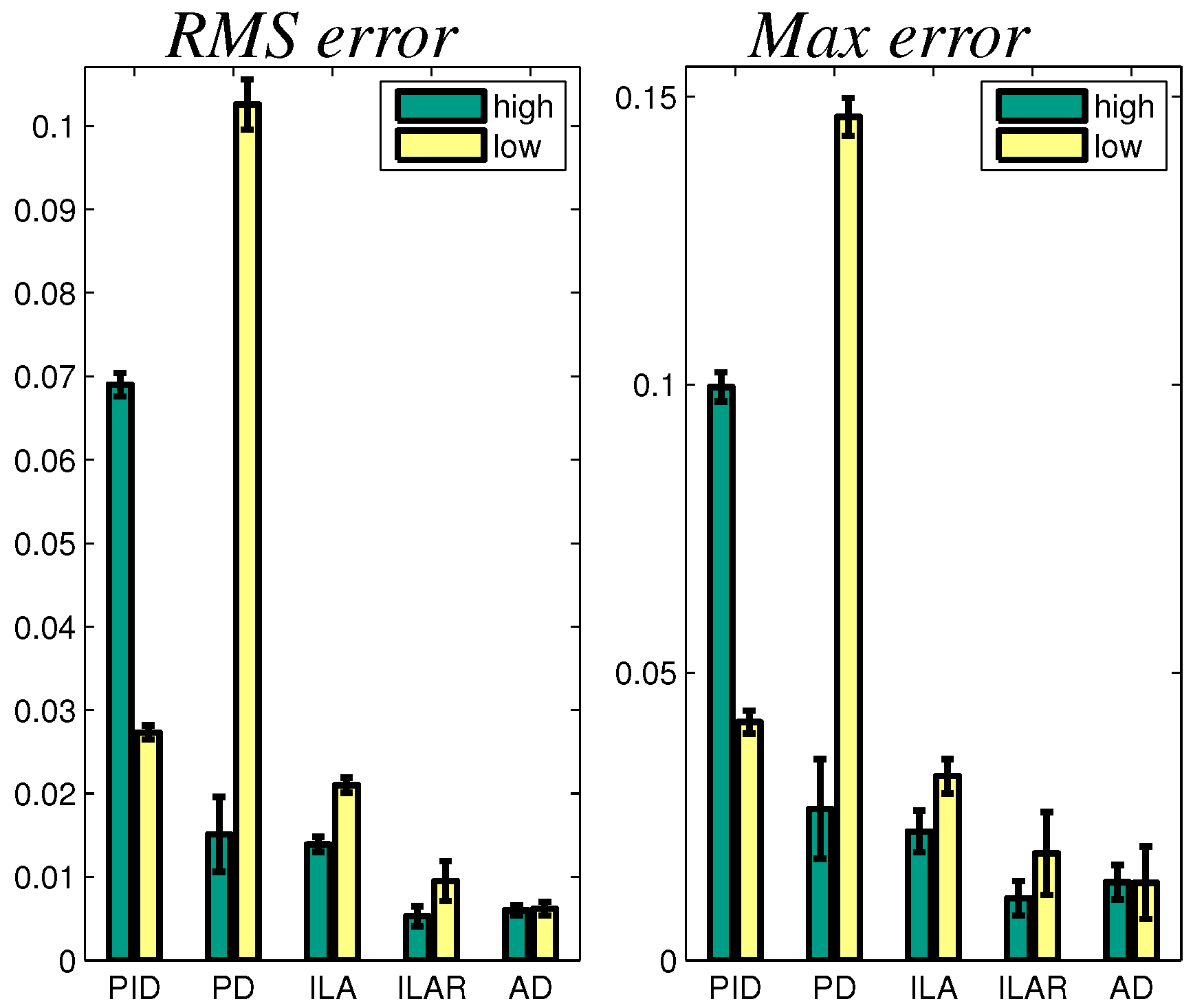
To quantitatively compare ILA, ILAR and adaptive algorithms, we considered the same kind of experiments described above (4-Hz sinusoidal torque tracking with an amplitude of 0.2 Nm), but we do separate tests for the high and low impedance conditions. The results are reported in Table 4 in terms of root mean square (RMS) and maximum error (Max). Due to the uncertain nature of pHRI, these indexes are computed for each reference period (We have a total of 240 periods for each controller, 120 in the high impedance condition and 120 in the low impedance condition) and considered as random processes with standard deviations and , respectively. As a result, the ILAR algorithm shows an evident improvement w.r.t. ILA, proving the effectiveness of embedding the internal model principle inside the sliding boundary. On the other hand, the adaptive controller seems to be only slightly better w.r.t. ILAR. The difference is even less significant if compared with the behavior of existing passivity-based solutions. the performance of which has been reported in Figure 13.
| High Impedance | Low Impedance | ||||||
|---|---|---|---|---|---|---|---|
| ILA | ILAR | AD | ILA | ILAR | AD | ||
| 13.9 | 5.3 | 6.0 | 21.0 | 9.5 | 6.2 | ||
| 0.3 | 0.4 | 0.19 | 0.3 | 0.8 | 0.27 | ||
| 22.4 | 10.8 | 13.6 | 32.0 | 18.6 | 13.5 | ||
| 1.2 | 1.0 | 1.0 | 1.0 | 2.4 | 2.1 | ||
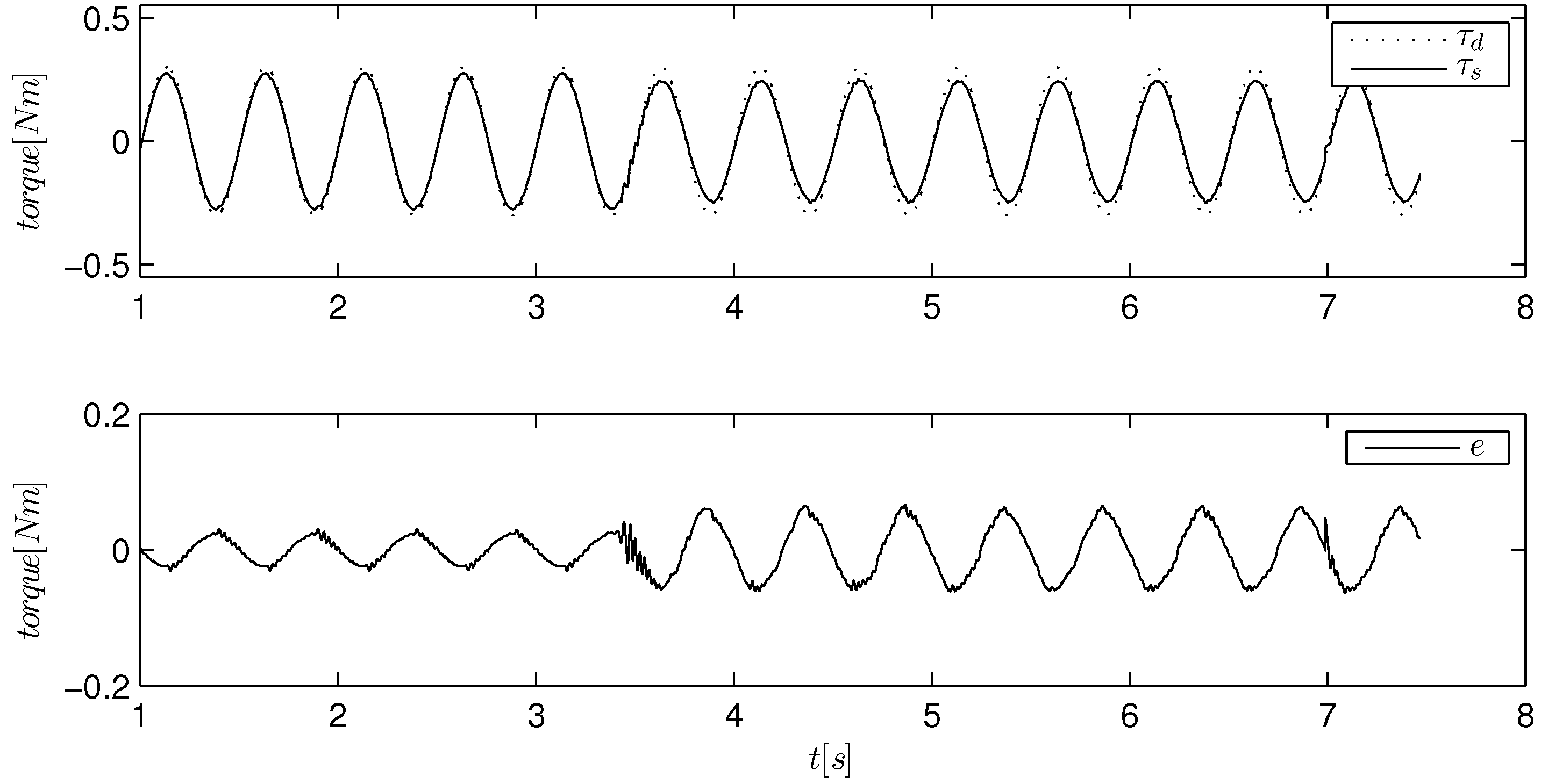
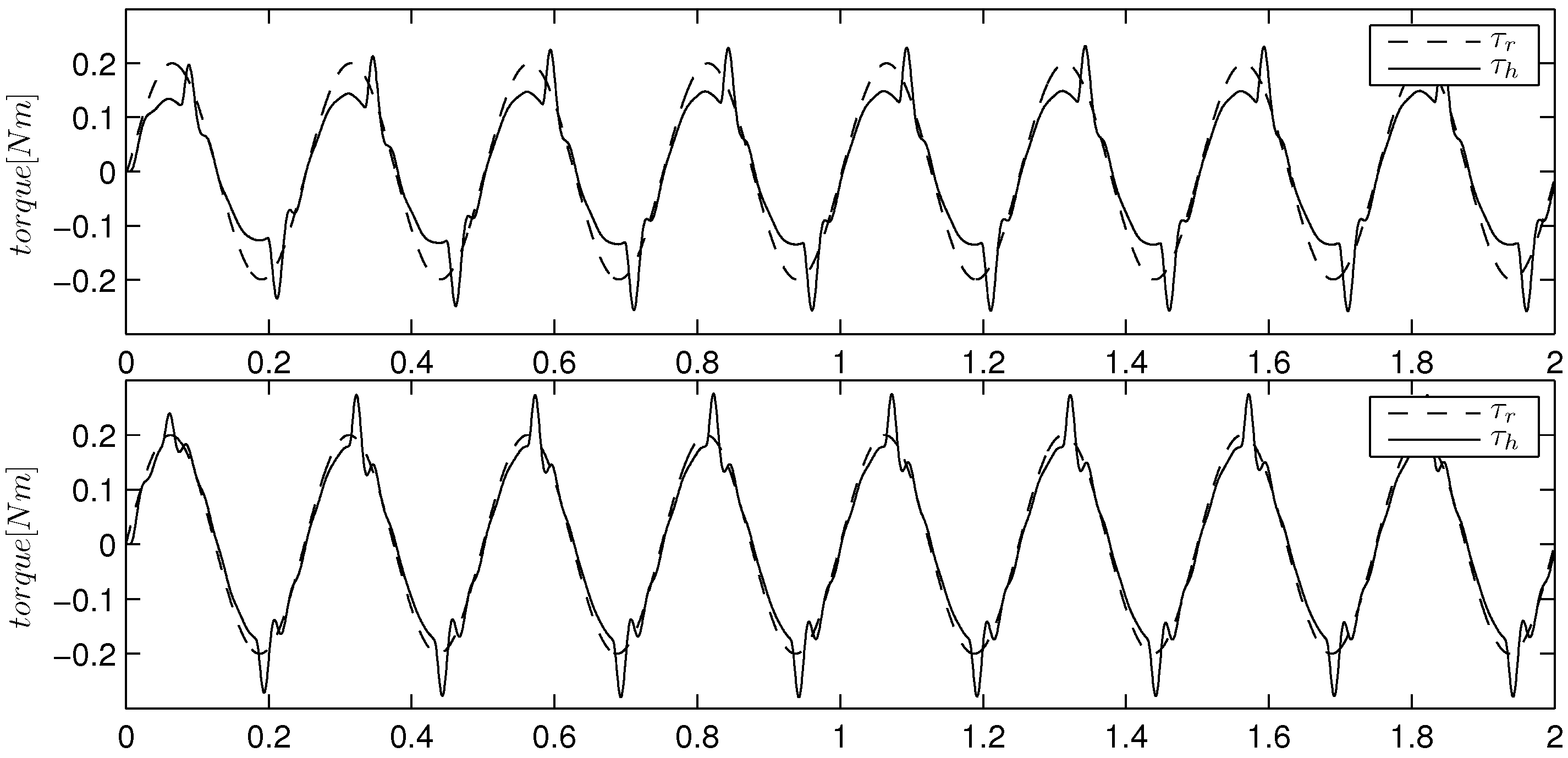
Finally we include a comparison between adaptive and ILAR algorithms during an intermittent impact test. In this experiment, we make the wood frame periodically hit a semi-rigid body, while it is tracking a sinusoidal torque reference. This situation usually represents a difficult control condition for robots, and to maintain low contact forces is usually challenging. The adaptive and sliding-mode algorithms exhibit a very different behavior, as shown in Figure 14. The adaptive controller acts by lowering its gains; thus, it reduces the impact force. As a consequence, the stability robustness increases at the cost of losing performance. On the other hand, the sliding-mode controller shows higher performance robustness with the side effect of higher impact forces.
Figure 13.
Graphical representation of the quantitative comparison with intervals to compare the performances in the high (green) and low (yellow) impedance conditions. The labels, PID and PD, are related to passive controllers, while AD indicates the adaptive controller.
Figure 13.
Graphical representation of the quantitative comparison with intervals to compare the performances in the high (green) and low (yellow) impedance conditions. The labels, PID and PD, are related to passive controllers, while AD indicates the adaptive controller.

Figure 14.
The response of the adaptive control (top) and ILAR algorithm (bottom) in an intermittent contact test.
Figure 14.
The response of the adaptive control (top) and ILAR algorithm (bottom) in an intermittent contact test.

6. Conclusions
In this paper, a sliding-mode solution for stable and accurate interaction control has been proposed, considering a series elastic actuator at the man-machine interface. We showed that integral sliding-mode allows fully predictable dynamics by avoiding the reaching phase, and it can improve the level of safety by assuring a bounded control input. We also proposed a solution to improve the accuracy of the linear approximation by introducing a simple task model. As a result, we achieve similar performance w.r.t adaptive control and also reduced chattering w.r.t. to second order SMC.
As a further development, we are currently investigating a robustification of adaptive control by means of SMC. This will ensure enhanced coupled stability, accounting for the presence of non-linear human dynamics and voluntary forces, and high accuracy, without the need of a task model.
A. Control Safety
Most of traditional controllers commonly adopted in robotics involve some risk of unsafe behavior when an anomalous event occurs. In case of unexpected contacts, temporary power failure, wrong system initialization or discontinuous control reference, the system can significantly deviate from the desired trajectory, generating a large control error [29]. Let us call control safety the control reaction to such a condition. A traditional control system can react with a sudden and excessive growth of controller internal energy due to the fact that most controllers employ either a high proportional gain, , or an integral gain, . During the error recovery process, the internal energy due to proportional action is quadratically related to the error deviation , whereas the integrator energy continuously increases unless the error goes to zero. Once we have an excessive control energy (which cannot be dissipated by the system), we get also into an undue control effort, which is a primary cause of unsafe behaviors. A well-known example is that of position-controlled robots, where high proportional gains are usually adopted and system dissipation is usually low [29]. Similar considerations apply to force control, where, in addition, we need to deal with environment uncertainties.
As a conclusion, if we aim at safety, force control should not only be robust to uncertainties, but should also reduce any proportional or integral action. This safety condition is satisfied in the case of integral SMC with equivalent control (19) and , which gives . One can note that the combination of Equations (5) and (19) is bounded, even if , providing limited . We highlight that the derivative term, , can be regarded as a dissipation; thus, it works at reducing the controller internal energy. The only risk with the error derivative can be due to discontinuous or abrupt changes in the reference signal, which can be easily avoided by using a pre-filter or a derivative roll-off.
B. Adaptive Force Control
This adaptive solution proposed in [18] considers an interaction model similar to that described in Section 3, but regards the environment as a second order linear system and online estimates its parameters. Given such an estimate, stability analysis can proceed using stability tools instead of passivity theory, providing convergence of both the force error and estimated parameters. In this approach, specifications can be given based on a second order model reference:
where represents the desired torque dynamics for in response to the reference input, , and parameters and are positive and chosen according to the desired responses of the controlled system. The proposed controller is defined as:
with adaptation dynamics given by:
where is the error with respect to the reference model (26) and is a measure of tracking performance. The parameter, ρ, determines the adaptation speed, and σ is a forgetting factor, which can be set arbitrarily small. The term, δ, is equal to , where ϵ is an arbitrarily small positive parameter.
Control stability can be proven in the sense of boundedness, i.e., the tracking error is guaranteed to converge inside a ball into the state space. Moreover, the ball dimension can be arbitrarily reduced by acting on the parameter, λ. This is formally stated and proven in [18].
Author Contributions
Andrea Calanca: SM theory, section 4 theory, experiments, manuscript writing.
Luca Capisani: SM theory, manuscript revision.
Paolo Fiorini: supervision, manuscript revision.
Conflicts of Interest
The authors declare no conflict of interest.
References
- Ekkelenkamp, R.; Veneman, J.; van der Kooij, H. LOPES: Selective Control of Gait Functions During the Gait Rehabilitation of CVA Patients. In Procedings of the 9th International Conference on Rehabilitation Robotics, Chicago, IL, USA, 28 June–1 July 2005; pp. 361–364.
- Herr, H.M.; Grabowski, A.M. Bionic ankle-foot prosthesis normalizes walking gait for persons with leg amputation. Proc. Biolog. Sci. 2012, 279, 457–464. [Google Scholar] [CrossRef] [PubMed]
- Lens, T.; Kunz, J.; Stryk, O.V.; Trommer, C.; Karguth, A. BioRob-Arm: A Quickly Deployable and Intrinsically Safe , Light-Weight Robot Arm for Service Robotics Applications. In Proceedings of the 41st International Symposium on Robotics, Munich, Germany, 7–9 June 2010; pp. 905–910.
- Duschau-Wicke, A.; von Zitzewitz, J.; Caprez, A.; Lunenburger, L.; Riener, R. Path control: A method for patient-cooperative robot-aided gait rehabilitation. IEEE Trans. Neural Syst. Rehabilit. Eng. 2010, 18, 38–48. [Google Scholar] [CrossRef] [PubMed] [Green Version]
- Pratt, J.; Chew, C.M.; Torres, A.; Dilworth, P.; Pratt, G. Virtual model control: An intuitive approach for bipedal locomotion. Int. J. Rob. Res. 2001, 20, 129–143. [Google Scholar] [CrossRef]
- Vallery, H.; van Asseldonk, E.H.F.; Buss, M.; van der Kooij, H. Reference trajectory generation for rehabilitation robots: complementary limb motion estimation. IEEE Trans. Neural Syst. Rehabilit. Eng. 2009, 17, 23–30. [Google Scholar] [CrossRef] [PubMed]
- Hogan, N. Impedance Control: An Approach to Manipulation: Part I,II,III. Journal of dynamic systems, measurement and control 1985, 107, 1–24. [Google Scholar] [CrossRef]
- Kong, K.; Member, S.; Bae, J. Control of Rotary Series Elastic Actuator for Ideal Force-Mode Actuation in Human-Robot Interaction Applications. IEEE/ASME Int. Conf. Mechatr. 2009, 14, 105–118. [Google Scholar] [CrossRef]
- Calanca, A.; Piazza, S.; Fiorini, P. Force Control System for Pneumatic Actuators of an Active Gait Orthosis. In Proceedings of the 2010 3rd IEEE RAS and EMBS International Conference on Biomedical Robotics and Biomechatronics (BioRob), Tokyo, Japan, 26–29 September 2010; pp. 849–854.
- Calanca, A.; Piazza, S.; Fiorini, P. A motor learning oriented, compliant and mobile Gait Orthosis. Appl. Bionic. Biomech. 2012, 9, 15–27. [Google Scholar] [CrossRef]
- Vallery, H. Stable and User-Controlled Assistance of Human Motor Function. Ph.D. Thesis, University of Munchen, Munich, Germany, 2009. [Google Scholar]
- Buerger, S.; Hogan, N. Relaxing Passivity for Human-Robot Interaction. In Proceedings of the 2006 IEEE/RSJ International Conference on Intelligent Robots and Systems, Beijing, China, 9–15 October 2006; pp. 4570–4575.
- Buerger, S.; Hogan, N. Complementary stability and loop shaping for improved human-robot interaction. IEEE Trans. Robot. 2007, 23, 232–244. [Google Scholar] [CrossRef]
- Colgate, E. The Control of Dynamically Interacting Systems. Ph.D. thesis, Massachusetts Institute of Technology, Cambridge, MA, USA, 1988. [Google Scholar]
- Hogan, N. Controlling impedance at the man/machine interface. In Proceedings of the International Conference on Robotics and Automation, Scottsdale, AZ, USA, 14–19 May 1989; pp. 1626–1631.
- Pratt, G.; Williamson, M.; Dillworth, P. Stiffness isn’t everything. In Proceedings of the Fourth International Symposium on Experimental Robotics, Stanford, CA, USA, 30 June–2 July 1995.
- Tagliamonte, N.L.; Accoto, D. Passivity Constraints for the Impedance Control of Series Elastic Actuators. J. Syst. Contr. Eng. 2013, 228, 138–153. [Google Scholar] [CrossRef]
- Calanca, A.; Fiorini, P. Human-Adaptive Control of Series Elastic Actuators. Robotica 2014, in press. [Google Scholar]
- Vallery, H.; Veneman, J.; van Asseldonk, E.H.F.; Ekkelenkamp, R.; Buss, M.; van Der Kooij, H. Compliant actuation of rehabilitation robots. IEEE Robot. Automa. Mag. 2008, 15, 60–69. [Google Scholar] [CrossRef]
- Pratt, G.A.; Willisson, P.; Bolton, C. Late motor processing in low-impedance robots: Impedance control of series-elastic actuators. In Proceedings of the American Control Conference, Boston, MA, USA, 30 June–2 July 2004; pp. 3245–3251.
- Markus, G.; Roman, M.; Konigorski, U. Model Based Control of Series Elastic Actuators. In Proceedings of the IEEE RAS/EMBS International Conference on Biomedical Robotics and Biomechatronics, Rome, Italy, 24–27 June 2012; pp. 538–543.
- Bae, J.; Kong, K.; Tomizuka, M. Gait Phase-Based Smoothed Sliding Mode Control for a Rotary Series Elastic Actuator Installed on the Knee Joint. In Proceedings of the American Control Conference, Baltimore, MD, USA, 30 June–2 July 2010; pp. 6030–6035.
- Utkin, V.I. Sliding Modes in Control and Optimization; Communications and Control Engineering; Springer-Verlag: Berlin, Germany, 1992; p. 286. [Google Scholar]
- Slotine, J.J.E.; Li, W. Applied Nonlinear Control; Prentice Hall: Englewood Cliffs, NJ, USA; Vol. 62, 1991; pp. 174–174. [Google Scholar]
- Damme, M.V.; Vanderborght, B. Proxy-based sliding mode control of a planar pneumatic manipulator. Int. J. Rob. Res. 2009, 28, 266–284. [Google Scholar] [CrossRef]
- Beyl, P.; Van Damme, M.; Van Ham, R.; Vanderborght, B.; Lefeber, D. Design and control of a lower limb exoskeleton for robot-assisted gait training. Appl. Bionic. Biomech. 2009, 6, 229–243. [Google Scholar] [CrossRef]
- Frisoli, A.; Sotgiu, E.; Procopio, C.; Bergamasco, M.; Rossi, B.; Chisari, C. Design and Implementation of a Training Strategy in Chronic Stroke with an Arm Robotic Exoskeleton. In Proceedings of the International Conference on Rehabilitation Robotics, Zurich, 29 June–1 July 2011; pp. 1127–1134.
- Kong, K. Proxy-based impedance control of a cable-driven assistive system. Mechatronics 2013, 23, 147–153. [Google Scholar] [CrossRef]
- Kikuuwe, R.; Yasukouchi, S.; Fujimoto, H.; Yamamoto, M. Proxy-Based Sliding Mode Control: A Safer Extension of PID Position Control. IEEE Trans. Rob. 2010, 26, 670–683. [Google Scholar] [CrossRef]
- Edwards, C.; Spurgeon, S. Sliding Mode Control: Theory And Applications; Taylor & Francis: London, UK, 1998. [Google Scholar]
- Bartolini, G.; Ferrara, A.; Usai, E. Chattering avoidance by second-order sliding mode control. IEEE Trans. Autom. Contr. 1998, 43, 241–246. [Google Scholar] [CrossRef]
- Levant, A. Higher-order sliding modes, differentiation and output-feedback control. Int. J. Contr. 2003, 76, 924–941. [Google Scholar] [CrossRef]
- Francis, B.; Wonham, W. The internal model principle of control theory. Automatica 1976, 12, 457–465. [Google Scholar] [CrossRef]
- Calanca, A.; Capisani, L.; Ferrara, A.; Magnani, L. MIMO closed loop identification of an industrial robot. IEEE Trans. Contr. Syst. Technol. 2011, 19, 1214–1224. [Google Scholar] [CrossRef]
- Calanca, A.; Capisani, L.; Fiorini, P.; Ferrara, A. Improving Continuous Approximation of Sliding Mode Control. In Proceedings of the 16th International Conference on Advanced Robotics, Montevideo, Uruguay, 25–29 November 2013.
- Pratt, G.A.; Williamson, M. Series Elastic Actuators. In Proceedings of the International Conference on Intelligent Robots and Systems, Pittsburgh, PA, USA, 5–9 August 1995; pp. 399–406.
© 2014 by the authors; licensee MDPI, Basel, Switzerland. This article is an open access article distributed under the terms and conditions of the Creative Commons Attribution license (http://creativecommons.org/licenses/by/3.0/).
Share and Cite
MDPI and ACS Style
Calanca, A.; Capisani, L.; Fiorini, P. Robust Force Control of Series Elastic Actuators. Actuators 2014, 3, 182-204. https://doi.org/10.3390/act3030182
AMA Style
Calanca A, Capisani L, Fiorini P. Robust Force Control of Series Elastic Actuators. Actuators. 2014; 3(3):182-204. https://doi.org/10.3390/act3030182
Chicago/Turabian StyleCalanca, Andrea, Luca Capisani, and Paolo Fiorini. 2014. "Robust Force Control of Series Elastic Actuators" Actuators 3, no. 3: 182-204. https://doi.org/10.3390/act3030182