
Quadcopter Trajectory Tracking Control Based on Flatness Model Predictive Control and Neural Network
College of Intelligent Systems, Science and Engineering, Harbin Engineering University, Habin 150001, China
*
Author to whom correspondence should be addressed.
Actuators 2024, 13(4), 154; https://doi.org/10.3390/act13040154
Submission received: 1 March 2024
/
Revised: 9 April 2024
/
Accepted: 11 April 2024
/
Published: 18 April 2024
(This article belongs to the Special Issue Fault-Tolerant Control for Unmanned Aerial Vehicles (UAVs))
Abstract
:In this paper, a novel control architecture is proposed in which FMPC couples feedback from model predictive control with feedforward linearization. The proposed approach has the computational advantage of only requiring a convex quadratic program to be solved instead of a nonlinear program. Feedforward linearization aims to overcome the robustness issues of feedback linearization, which may be the result of parametric model uncertainty leading to inexact pole-zero cancellation. A DenseNet was trained to learn the inverse dynamics of the system, and it was used to adjust the desired path input for FMPC. Through experiments using quadcopter, we also demonstrated improved trajectory tracking performance compared to that of the PD, FMPC, and FMPC+DNN approaches. The root mean square (RMS) error was used to evaluate the performance of the above four methods. The results demonstrate that the proposed method is effective.
1. Introduction
Quadcopters have experienced a substantial surge in popularity. The quadcopter-like Parrot AR.Drone [1] is presently employed in various applications, including but not limited to tasks such as inspection [2], search and rescue missions [3], mapping operations [4], and photography. Historically, PID controllers have been chosen for their simplicity and satisfactory performance. However, they may not offer optimal performance when dealing with diverse trajectories that have significant curvature. This research aims to develop a model predictive controller (MPC) [5] that addresses the limitations of proportional–integral–derivative (PID) controllers and offers enhanced trajectory-tracking capabilities for quadcopters. An MPC is an optimum control strategy that efficiently solves an optimization problem in real-time. Current real-time NMPC frequently performs only one iteration of a sequential quadratic program (SQP) with Gauss–Newton approximation, resulting in a suboptimal NLP solution [6,7]. The primary goal of an MPC is to calculate the most favorable control input by considering the current state and a desired set of future states. Various versions of MPC controllers are proposed in the literature. The methodology employed in this study is like the strategy proposed by M. Greeff and A. Schoellig in [8]. It incorporates the differential flatness characteristic of quadcopters combined with feedforward linearization and is commonly known as flatness model predictive control (FMPC).
MPCs outperform PID controllers for quadcopter applications. However, they still rely on a correct underlying system model, which may be challenging to accomplish in practice. To understand the unmodeled dynamics of the system, a DenseNet was trained using a methodology similar to that described in a previous study [9]. In that study, the network successfully learned the inverse dynamics of the system and was subsequently utilized to modify the desired trajectory employed by model predictive control (MPC).
Model predictive control has various versions, including nonlinear MPC [6], which addresses the non-convex, nonlinear optimization problem by employing direct nonlinear dynamics. The methodology is characterized by a high computation and a susceptibility to converging towards local minima. An alternative method is linear MPC [5], which involves linearizing the nonlinear model, bringing up a convex problem. This approach is simpler than nonlinear MPC. However, it suffers from performance drawbacks because of linearization. J.A. Primbs et al. [10] integrated feedback linearization with MPC. According to [11], coupling linear MPC with feedback linearization requires nonlinear term cancellation, making its robustness to noise, parameter uncertainty, and disturbances difficult to assess. They suggest including plant uncertainty in MPC+FBL (MPC and feedback linearization). MPC+FBL lacks robustness by failing to account for known input time delays. This approach eliminates nonlinear components through the feedback linearization process, leading to an optimization problem for MPC that can be formulated as a linear system of equations. This method is advantageous because it allows for the resulting optimization problem to be formulated as a quadratic program known for its computing efficiency. Furthermore, linearization around a fixed point is unnecessary. Typically, it is observed that the feedback linearization approach is subject to robustness problems. Thus, utilizing MPC with feedforward linearization is a potentially more effective method [8] in which the optimal future states are used to cancel the nonlinear terms. This requires dealing with the optimal future states obtained during the optimization process to overcome the influence of nonlinear components through a feedforward mechanism. Feedforward linearization aims to address the robustness challenges that arise from feedback linearization. These challenges may occur due to uncertainties in the parametric model, leading to the imperfect cancellation of poles and zeros [12]. For example, implementing feedforward linearization in the ball-plate experiment enhanced tracking performance compared to feedback linearization [13]. Due to the coupling of linear MPC with feedback, linearization requires nonlinear term cancellation, making its robustness to noise, parameter uncertainty, and disturbances difficult to assess. Feedforward linearization aims to overcome the robustness issues of feedback linearization, which may be the result of parametric model uncertainty leading to inexact pole-zero cancellation. The proposed methodology in this paper combines feedforward linearization with MPC, improving robustness and tracking performance.
The authors of [14] mainly investigate real-time optimal trajectory generation techniques, which enable dynamic systems in engineering applications to perform optimal trajectory planning under constraints. They discuss the concept of differential flatness and its application in trajectory generation. They describe the controllability and observability of a system. If a system is differentially flat, then all of its states and inputs can be parameterized by its outputs and a finite number of their derivatives. This implies that the dynamic behavior of the system can be fully captured by a finite-dimensional representation of the outputs, thereby simplifying the trajectory generation problem. The FMPC described in [8] employs differential flatness, a feature of many physical systems, such as cranes, cars with trailers, and quadrotors [15]. Differential flatness separates a nonlinear model into linear dynamics and nonlinear transformations. This characteristic is applicable in both feedback and feedforward linearization [12]. To put it in basic terms, a method is differentially flat if its state can be represented in terms of a flat output and its derivatives, which are not related to each other using a differential equation [15,16]. This problem is simplified by expressing the state in its flat counterpart, as the system formulation in the flat output space is linear. This allows for the integration of all of the nonlinear components into the feedforward linearization process.
MPC relies on an underlying accurate system model, which is hard to achieve because modeling aerodynamic drag, vibrations, and so on for a quadcopter is difficult. Much work can be found in the literature to learn the unknown dynamics of robotic systems. N. Petit, Mark B. Milam, and R.M. Murray [17] proposed a computationally efficient technique for the numerical solution of optimal control problems. This method utilizes tools from the nonlinear control theory to transform the optimal control problem to a new, lower-dimensional set of coordinates. Through numerical examples, it is shown that increasing the use of inverse mapping significantly improves the execution speed without sacrificing the convergence rate. Machine learning approaches have been successfully integrated into control system designs in several instances, leading to improved tracking performance in the presence of unpredictable environments [18,19,20,21]. Examples of these machine learning techniques include but are not limited to Gaussian Processes (GPs), ILC, and DNNs [22], among others. In [23], a recurrent neural network (RNN) was introduced that learned the dynamics of automated food slicing. The network was employed along with the MPC optimization loop to control the actions of a robot slicing different kinds of food items with a knife. Despite its effectiveness, the strategy incurs significant computational costs since the approach needs to learn the system’s dynamics from the beginning. In the case of a quadcopter, the conventional dynamics model remains an accurate representation of the actual system. Consequently, abandoning this model and learning the dynamics from the start would be inefficient.
A more effective strategy is to enhance and refine the existing model of the system, as suggested in [8], by training a deep neural network (DNN) to learn the inverse dynamics of a quadcopter following an impromptu trajectory. So, the deep neural network (DNN) was able to learn the inverse dynamics of a quadcopter and was used to adapt the desired flight path employed by MPC. Early review publications [24,25] explain how DNNs can be coupled with control approaches like predictive and adaptive control to account for system uncertainties and non-idealities. Numerous studies have demonstrated the effectiveness of using DNNs in various control applications. In [26], it was shown that DNNs can help linear quadratic regulators (LQR) manage trajectory tracking by approximating unmodeled quadrotor dynamics. In [27] and related studies in the literature, DNNs were employed to account for model uncertainty in manipulator impedance control. The trained DNN was then used to adjust the input to the controller to improve performance. However, during the training process of a DNN, the employment of gradient descent methods can often result in the problem of gradients converging towards zero, which can impede training to a standstill, particularly as the number of network layers grows. Consequently, the premature termination of training activity occurs, resulting in suboptimal parameter optimization. The solution to this problem is adopting a DenseNet [28], which is a feedforward convolutional neural network (CNN) architecture that links each layer to every other layer, incorporates skip connections, and effectively prevents the issue of premature optimization termination. Employing DenseNet guarantees that the parameter gradients do not converge to values extremely close to zero while undergoing optimization. This allows for the optimization of network parameters towards suitable optimal solutions.
We proposed an efficient controller to control a quadcopter and obtained a reliable trajectory-tracking performance. The significant contributions of this article are as follows:
- (1)
- This study proposes a novel control architecture in which FMPC couples feedback from model predictive control with feedforward linearization to provide a more reliable trajectory-tracking performance.
- (2)
- To further improve the performance of the above control architecture, a DenseNet was trained to learn the inverse dynamics of the system, which was used to adjust the desired path input to FMPC.
- (3)
- DenseNet and the feedforward linearization combined with feedback model predictive control both form a larger feedback system to improve the control robustness and trajectory-tracking performance of the quadcopter.
This paper is organized as follows: Section 2 explains the problem statement, Section 3 presents the background knowledge, and Section 4 describes the methodology of using MPC and learning the dynamics. Finally, Section 5 presents the experimental results and a discussion of the proposed techniques. Section 6 concludes the paper and describes future work objectives.
2. System Description
The mathematical model developed in the above section can be represented in a state-space form, , where the state and the input are given by
where , , and represent the linear position of the quadcopter; , , and correspond to the quadcopter’s roll, pitch, and yaw angles; is the commanded velocity in the z direction; is the commanded roll angle; is the commanded pitch angle; and is the commanded yaw rate.
The system model is given by
where , and . Note that the system’s response to the inputs was modeled using first-order differential equations, which worked fine with the simulation environment. The values of the time constants were identified by observing the system’s step response.
We consider the hover to be , where we assume that our current yaw angle remains constant at each time step.
Our control system comprises a low-level onboard controller and an MPC outer-loop controller. The MPC controller is capable of sending commands: .
Here represents the desired velocity in the z direction, is the desired roll angle, is the desired pitch angle, and is the desired yaw rate.
We begin by performing a system identification process to enhance the trajectory tracking accuracy. This process is similar to the method described in reference [29], allowing us to estimate the inner-loop attitude dynamics.
The symbols and indicate time constants. and show defined gains, and the angles , , and correspond to the quadcopter’s roll, pitch, and yaw angles. In contrast to [28], we refrain from transmitting a direct thrust command, . As a result, we make a comparable system identification to calculate the z-velocity dynamics using a second-order response with a time delay (td) of 0.1 s as follows:
where , , and are known time constants.
3. Background Knowledge
A nonlinear system model (3) is considered differentially flat if it exists , consisting of differentially independent components (meaning they are not related to each other through a differential equation), and the following condition is satisfied [15]:
where , and denote smooth functions, and represent the maximum orders of derivatives, and are required to explain the system, and is referred to as the flat output.
Every system that exhibits differential flatness can be mathematically described using a Brunovsky state (also known as a flat state):
It should be noted that represents the highest order derivative of found in Equation (8).
By using the state transformation between the flat state z and state x, derived by the differentiation of Equation (6) and utilizing Equation (7), we may convert Equation (2) into the standard form.
where represents a smooth function formed by the process of the transfor mation. Note that is the highest derivative of after times differentiating in Equation (6). The flat input, , is defined as follows:
By applying the explanations provided in (9) and (11), we rephrase (10) as follows:
where The linear flat model is denoted as (12). By replacing the definitions in Equations (9) and (11), we may rephrase Equation (8) as follows:
The following theorem is derived from reference [12]: Take into account a desired path in the flat output , together with a matching desired flat state (achieved by replacing the variable with the expected value of in Equation (9)) and desired flat input (obtained by replacing the variable with the desired value of in Equation (10) and Equation (11)). Given , and given that the nominal control, , is applied to a differentially flat system of Equation (2), provided that , it leads to a linear system through a change in coordinates, as expressed in Equation (12).
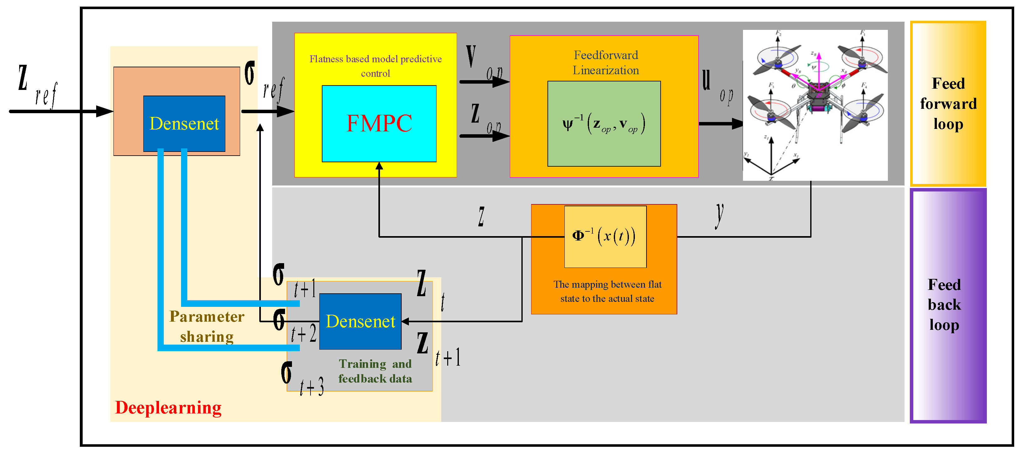
Theorem 1 enables trajectory generators or controllers to concentrate solely on the comparable linear flat model, as shown in our suggested approach depicted in Figure 1. The trajectory generator or controller produces the appropriate flat state and flat input as the output. These outputs can then be processed through inverse transformation (14) to counteract the system’s nonlinear component (13). Feedforward linearization fundamentally differs from feedback linearization by utilizing the desired flat state from Equation (14) instead of the measured flat state in the inverse term.
4. Methodology
The proposed method of coupling feedforward linearization and MPC, as seen in Figure 1, uses the linear flat model in a feedback MPC. The MPC outputs the flat state and flat input, which are then fed through the inverse term. Then, the result of feedforward linearization outputs to the quadcopter. The actual state of the quadcopter is mapped to a flat state, and the flat state is used as feedback for the controller. A DenseNet module is added to the FMPC architecture to adjust the reference inputs to the feedback control system. The DenseNet receives the current flat state and the future flat state as inputs. The DenseNet produces flat outputs that specify the desired trajectory input for the MPC controller.
4.1. Differential Flatness Formulation
This section presents some necessary formulations that rely on the differential flatness property of quadcopters. Note that we direct the reader to read [16] for more details about the characteristics of differential flatness. Below is a summary of this property.
Differential flatness means that the state and input ((1) and (2)) can be expressed in terms of a flat output and its derivatives. The flat output is defined as
and the flat state and flat input are defined as
The mapping between the flat state (16) and the actual state (1) is expressed below:
where is the gravitational constant; note that in the formulation shown above in (17), was assumed to be zero.
The mapping between the input, , from the flat state and flat input is provided as follows:
Below, and are given; note that their time derivatives were computed using the chain rule.
The entire system can be represented as a linear system by using the flat state and input in the following discretized form:
4.2. Flatness-Based Model Predictive Control
Based on the formulation of the system in the flat space (Equation (22)), the MPC optimization problem can be resolved by employing a quadratic cost function, similar to the approach described in reference [8]:
where is a positive semi-definite matrix that weighs the error with our reference trajectory. is positive-definite and regulates both the size and change in the inputs .
It should be noted that C is a permutation matrix consisting of ones and zeros, and it selects the flat output values from the flat state.
The above issue can be expressed as a quadratic program:
where .
The optimal input can then be determined by using Equation (19) and utilizing the optimal flat state and input obtained from the optimization problem :
4.3. Improvement via Learning
To enhance the accuracy of trajectory tracking for FMPC, a DenseNet was trained to effectively capture the inverse dynamics of the system. Figure 1 demonstrates the process of the DenseNet, where it feeds the reference trajectory as the input and generates a modified course with uniform or flat outputs . The concept is that the DenseNet will change the desired path to improve the overall tracking performance.
To provide a thorough explanation of the architecture and its underlying reasoning, we referred to Figure 2 and evaluated the following aspects:
- Assumptions: The DenseNet does not include modeling of the z and yaw directions to simplify the model. Only the x and y axes are taken into account.
- Inputs: The DenseNet receives the current flat state and the future flat state as inputs. Observing the x and y values relative to the position of is essential. This feature renders the neural network insensitive to the position of the input.
- Outputs: The DenseNet produces flat outputs that specify the desired trajectory input for the MPC controller. The value of N is either equal to or less than the prediction horizon of the MPC. Once again, all of the output values for x and y are relative to . So, to obtain the actual coordinates, the values are added back.
- Concept: Based on the current state and the desired future state , the DenseNet generates the optimal sequence of flat outputs to reach the desired future state . Consequently, the DenseNet learns inverse dynamics, and it refers to the inverse mapping from the input to the output. The input consists of the desired trajectory of MPC along with the current state , and the output is the future state .
- Training: The network is trained using a reference trajectory, , as shown in Figure 1. The resulting flat states, , are recorded. The flat states will serve as the inputs during the training phase, whereas will serve as the training labels. So, the neural network undergoes training using a supervised learning fashion.
- Inference: For an entire trajectory in a flat space , each pair of consecutive states in this trajectory feeds into the DenseNet. The DenseNet then produces N flat outputs , which are then recorded. At each time step t, the collected values are averaged and stored to create the reference trajectory .
The value of ‘N’ is essential as it determines the number of flat outputs generated by the neural network. Ideally, the value of ‘N’ should be the same as the prediction horizon of the MPC. However, this approach is inefficient, requiring the neural network to be more extensive. Only the initial reference states considerably impact the subsequent input to the quadcopters. States distant in the future have a diminished effect on the current input. Therefore, opting for N as ‘1’ results in unsatisfactory outcomes due to the neural network’s limited capacity for expressiveness. The value of N is selected as ‘3’, providing a balance between the two extremes and satisfactory results.
5. Experiment Results
5.1. Experiment Introduction
Various trajectories were constructed with varying degrees of aggression to evaluate the efficacy of the suggested architecture. The flight routes are designed to prevent abrupt changes in location, ensuring a smooth trajectory in the quadcopter’s input area [16]. These trajectories were selected based on their benchmark performance, which has set a standard for quadcopters. Minimum snap trajectories are generated by selecting an initial and final state and a sequence of waypoints connecting them. Ultimately, ninth-degree polynomial segments are utilized to establish connections between these waypoints. The optimization problem collectively solves the coefficients of the polynomial components.
The polynomial formulation is given as follows:
where is the total time assigned for the jth segment of the path. Note that dividing t by helps improve the numerical stability of the solution. The problem can then be formulated as a constrained quadratic program as follows:
where are the coefficients of the polynomial segments, and are the derivatives at the endpoints.
Three different minimum snap trajectories were generated with increasing levels of aggressiveness, with flight route ‘3’ being the most aggressive.
Before the experiments, a system identification step was executed where the system was subjected to a step input in the , , and directions. The time constants were 1.0, 2.4, and 2.4, respectively.
A PD controller coupled with feedback linearization was set up for comparison purposes. The dynamics in the x and y directions were modeled as a second-order system, and the tuned and gains were found to be ‘1’ and ‘8’, respectively. The z and yaw directions were modeled as first-order systems with a value of ‘10’. Note that a sufficient amount of effort was spent tuning the gains. However, there was no guarantee that they were optimal, as they could be further improved with more tuning.
For the FMPC controller, the model predictive loop was run at 10 Hz, with a prediction horizon of 20 time steps. Attempts to increase the prediction horizon to values higher than that have led to very low running frequencies, which caused instability. All quadratic programs were solved using the CVXOPT library in Python.
5.2. Training the DenseNet
To train the DenseNet, the flight routes shown in Figure 3 were used to compile a dataset. For each trajectory, the quadcopter performed 20 loops (10 in the reverse direction), resulting in 12,332 training/label tuples. The dataset was then normalized to avoid instability during training. The normalization coefficients were also stored to rescale the output from the neural network during inference. The direction of flight follows the direction of arrows.
The hidden layers of DenseNet consist of five layers and the same structures; each layer has 30 neurons and ReLU activations [30]. The root mean square error was used as the loss function, and Adam [31] was the optimizer chosen. The network was trained for 60 epochs with a batch size of 10.
The error function for each task is defined as the root mean square (RMS) error of N pairs of (x,y,z) coordinates sampled at 7 Hz, and the DenseNet feedback loop sampling rate between the desired trajectory, , and the observed trajectory, is determined as follows:
where is the Euclidean norm, while and are the position coordinates sampled at the time step from the desired trajectory and the observed trajectory , respectively. The quadrotor in the experiment repeats each task with and without the aid of the trained DenseNet.
Note that the selected trajectories for training had relatively mild maneuvers compared to some of the flight routes used in experimentation. That is because when attempting to train with more aggressive trajectories, the system experienced unfavorable fluctuations in the training dataset. Instead, relatively stable and well-conditioned flight routes were used for training, and their generalization to more aggressive trajectories was observed.
5.3. Results
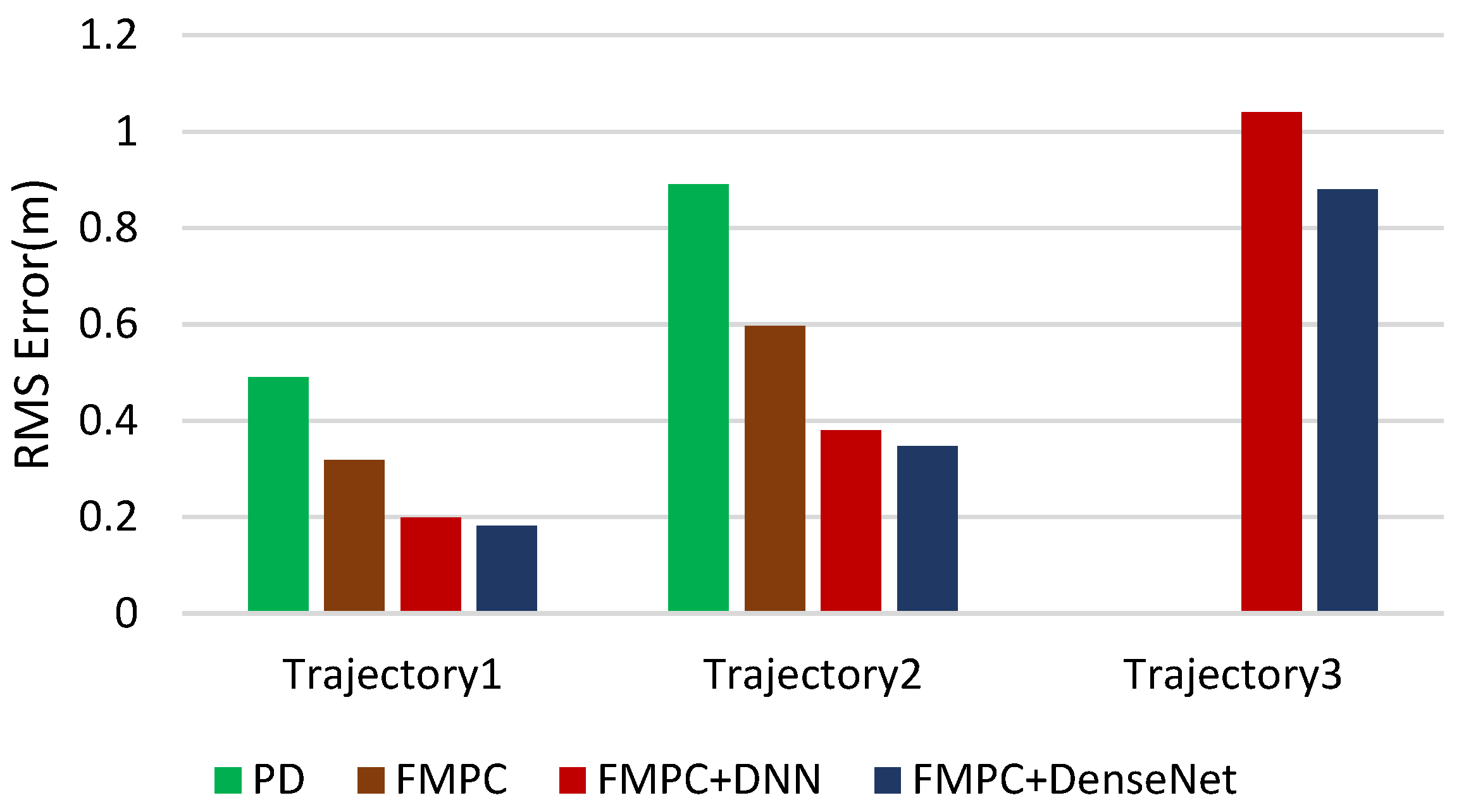
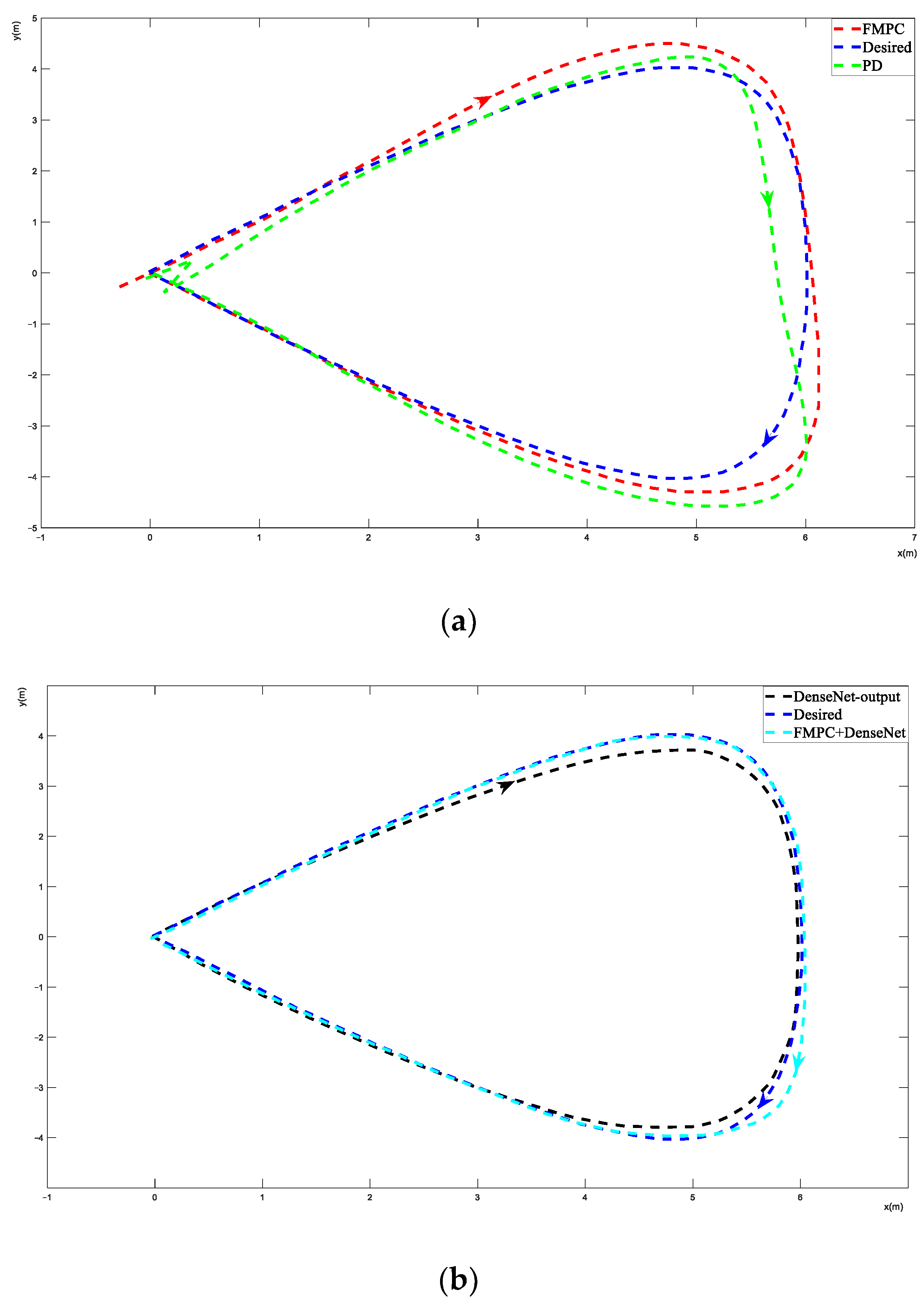
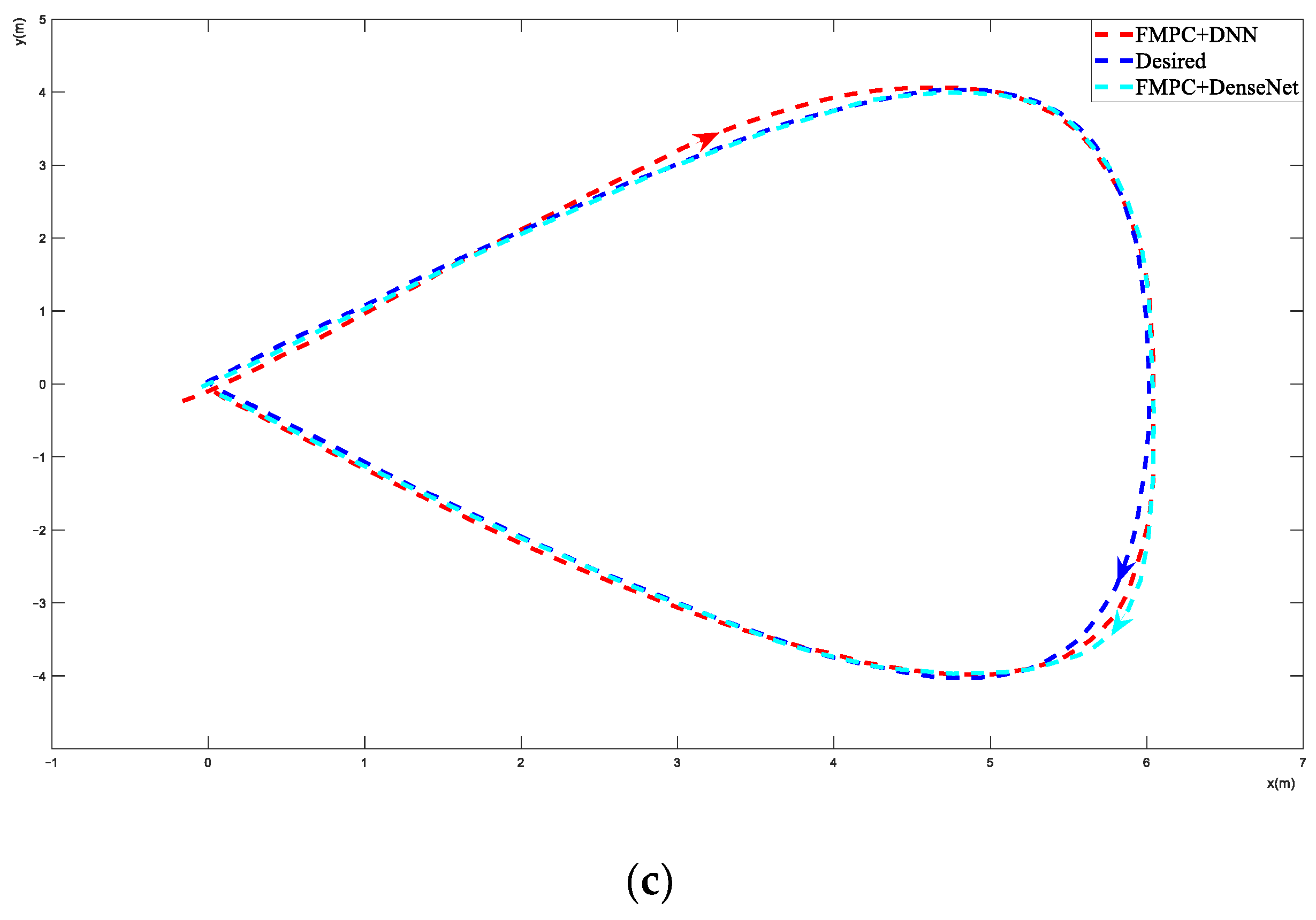
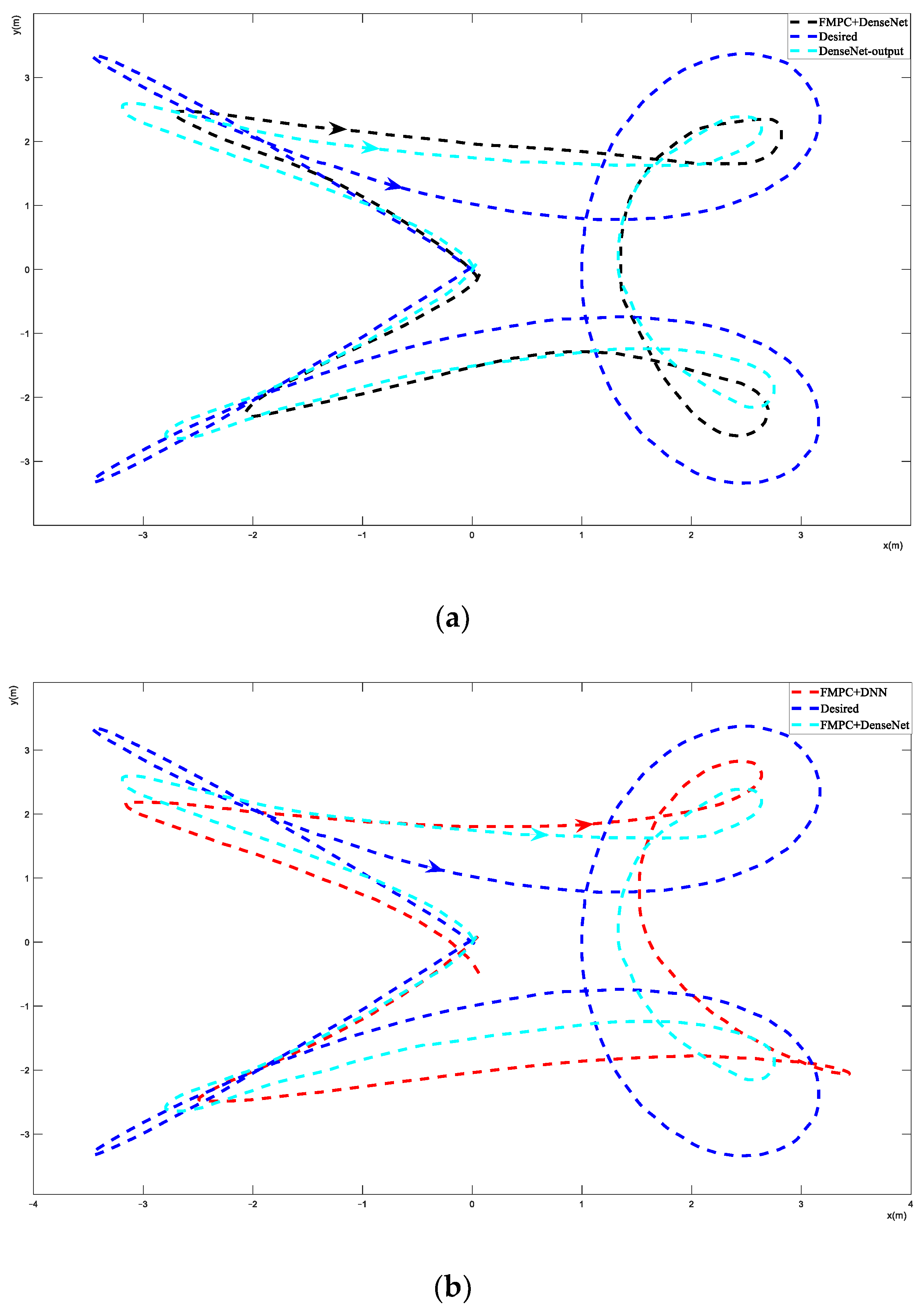
Figure 4 shows that the FMPC (without DNN and DenseNet) provides better trajectory tracking performance than the PD controller and has a 35% improvement on average. Figure 5a and Figure 6a depict figures of the resulting trajectories from the FMPC and PD controllers for trajectories 1 and 2, respectively. It is worth noting that the system has an unaccepted control error for trajectory 3 (the most aggressive) and cannot track this trajectory well when using the FMPC and PD control methods. That is because no constraints were imposed on the inputs when solving the MPC optimization problem and when generating the minimum snap trajectories. Therefore, the inputs were allowed to grow unboundless, in some cases exceeding the controllability range of the quadcopter (which is what happened with trajectory 3). The direction of flight in Figure 5, Figure 6 and Figure 7 follows the direction of arrows.
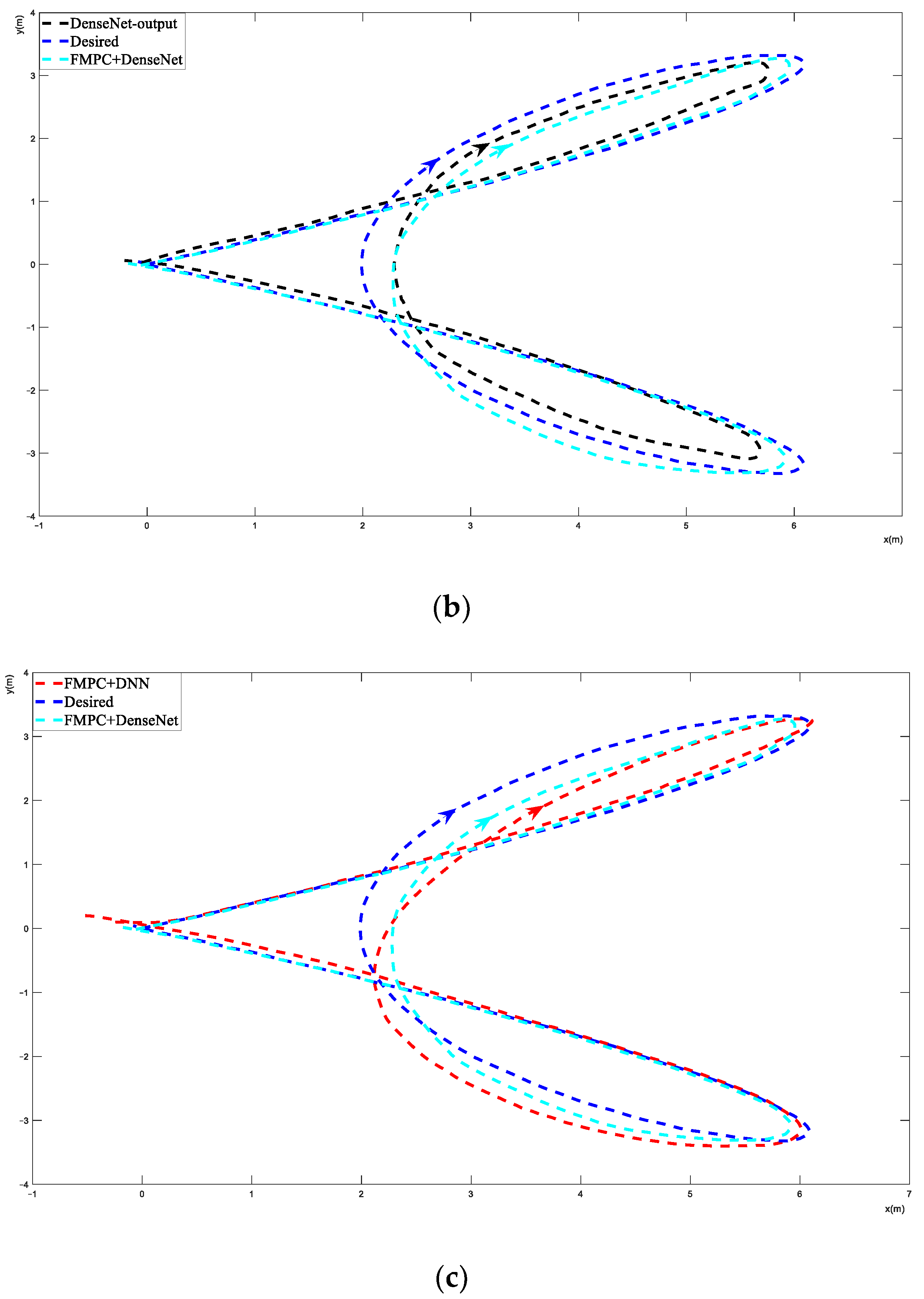
Figure 5a shows the PD and FMPC performance of trajectory 1; both PD and FMPC experience a noticeable drift from the desired trajectory. Figure 5b shows the DenseNet-output and FMPC+DenseNet performance of trajectory 1. The DenseNet output is the path, and it hopes FMPC adjusts its path to the desired path. Figure 5c shows the FMPC+DNN and FMPC+DenseNet performance of trajectory 1; both methods have a good performance, but it can be seen that FMPC+DenseNet achieved a more effective tracking performance.
Figure 6a shows that the PD method has a very unstable trajectory, and the FMPC method has an overshoot trajectory. Both PD and FMPC experience a significant amount of drift from the desired trajectory. Figure 6b presents the FMPC+DenseNet path and the adjusted desired path, which is the output of the DenseNet. As seen in Figure 6c, FMPC+DNN and FMPC+DenseNet achieve a more reasonable tracking performance, but FMPC+DenseNet has a more stable path than FMPC+DNN.
Figure 7 shows the FMPC+DNN and FMPC+DenseNet performance of trajectory 3. Both PD and FMPC have serious and unaccepted control errors and are not able to track this trajectory well. So, the figures of PD and FMPC are not listed. In Figure 7a, the black line presents the DenseNet output, which is the adjusted desired path. In Figure 7b, it can be seen that both FMPC+DNN and FMPC+DenseNet were able to track trajectory 3 in a stable state. We can see that FMPC+DenseNet has better performance than FMPC+DNN, and FMPC+DNN has an overshoot area with high curvature.
As can be seen in Figure 5a and Figure 6a, FMPC (without the DNN and DenseNet) always seemed to overshoot the desired trajectory at areas of high curvature. The reason for that could be that the MPC optimization loop might not be running at a high enough frequency, and the prediction horizon might not be sufficiently long. Also, the quadcopter might be reaching the limits of its controllability.
When the DNN and DenseNet are combined with FMPC, the trajectory tracking performance has improvements of 59% and 62% over the PD scenario, respectively, and improvements of 37% and 41% over FMPC for trajectories 1 and 2. Figure 5b and Figure 6b show figures of the outcomes for trajectories 1 and 2, respectively, with the black line representing the altered desired trajectory (DenseNet output) that is fed to the FMPC controller. For trajectories 1 and 2, FMPC+DenseNet has improvements of 3% and 4% over FMPC+DNN. For trajectory 3, although the PD and FMPC controllers resulted in instability, the FMPC+DNN and FMPC+DenseNet architectures resulted in reliable tracking, but that was at the cost of significant tuning to the original desired trajectory (as seen in Figure 7). It can be seen in Figure 4 that FMPC+DenseNet has a better performance than FMPC + DNN by about 11%. Hence, we can see that the DNN and DenseNet have learned to adjust the desired path by always pulling it inwards into the direction of curvature, with the amount of pull being proportional to the magnitude of velocities and accelerations. For example, by comparing the output of the DenseNet for trajectory 1 vs. trajectory 3, the amount of offset is much more significant in trajectory 3 since it requires movement at much higher velocities and accelerations. From Figure 7b, we can see that FMPC+DNN has a larger overshoot than FMPC+DenseNet. FMPC+DenseNet has a more stable trajectory, and the DenseNet has essentially learned that the quadcopter always overshoots areas of high curvature, so it pulled the desired trajectory in to compensate for this overshoot. So, the FMPC+DenseNet method performs better than FMPC + DNN and has a more stable trajectory. The DenseNet method offsets the disadvantage of a DNN and offers a good desired path for FMPC.
6. Conclusions
This study utilized a flatness-based model predictive controller (MPC) to regulate the movement of a quadcopter within a simulated environment. The controller’s performance surpasses that of a typical PD controller, resulting in a more reliable trajectory-tracking performance. To enhance the performance of FMPC, a DenseNet was trained to learn the inverse dynamics of the system. The network was then utilized to modify the desired path input for FMPC. When the controller faced potential instability without a DenseNet in FMPC, it ensured steady tracking and enhanced the tracking accuracy. Future research could evaluate the suggested framework under various model perturbations, such as gusty weather conditions. Moreover, optimizing the FMPC can enhance the controller’s prediction horizon, enhancing overall performance. Finally, the quadcopter’s inputs might be limited throughout the process of solving the MPC optimization problem and creating the minimum snap trajectories to ensure the safe operation of the quadcopter.
Future research could entail augmenting the training dataset for the DenseNet by incorporating a more comprehensive range of trajectories and evaluating the suggested framework under various model perturbations, such as gusty weather conditions. Moreover, optimizing the FMPC can enhance the controller’s prediction horizon, enhancing overall performance. Finally, the quadcopter’s inputs might be limited throughout the process of solving the MPC optimization problem and creating the minimum snap trajectories to ensure the safe operation of the quadcopter.
Author Contributions
Conceptualization, Y.L. and Q.Z.; methodology, Y.L.; software, Y.L.; validation, Y.L. and A.E.; formal analysis, Y.L. and A.E.; investigation, Y.L.; resources, Y.L.; data curation, Y.L.; writing—original draft preparation, Y.L.; writing—review and editing, Y.L.; visualization, Y.L.; supervision, Q.Z.; project administration, Q.Z.; funding acquisition, Q.Z. All authors have read and agreed to the published version of the manuscript.
Funding
Funding was provided by the National Natural Science Foundation of China with project grant number 52171299.
Data Availability Statement
All data are contained within the article.
Conflicts of Interest
The authors declare no conflicts of interest.
References
- Bristeau, P.; Callou, F.; Vissiere, D.; Petit, N. The navigation and control technology inside the ar. drone micro uav. IFAC Proc. 2011, 44, 1477–1484. [Google Scholar]
- Bircher, A.; Kamel, M.; Alexis, K.; Oleynikova, H.; Siegwart, R. Receding horizon path planning for 3D exploration and surface inspection. Auton. Robot. 2016, 42, 291–306. [Google Scholar] [CrossRef]
- Rudol, P.; Doherty, P. Human body detection and geo localization for UAV search and rescue missions using color and thermal imagery. In Proceedings of the IEEE Aerospace Conference, Big Sky, MT, USA, 1–8 March 2008; pp. 1–8. [Google Scholar]
- Han, J.; Chen, Y. Multiple UAV Formations for Cooperative Source Seeking and Contour Mapping of a Radiative Signal Field. J. Intell. Robot. Syst. 2013, 74, 323–332. [Google Scholar] [CrossRef]
- Bangura, M.; Mahony, R. Real-Time Model Predictive Control for Quadrotors. IFAC Proc. Vol. 2014, 47, 11773–11780. [Google Scholar] [CrossRef]
- Wang, Y.; Boyd, S. Fast Model Predictive Control Using Online Optimization. IEEE Trans. Control. Syst. Technol. 2010, 18, 267–278. [Google Scholar] [CrossRef]
- Houska, B.; Ferreau, H.; Diehl, M. ACADO toolkit—An open source framework for automatic control and dynamic optimization. Optim. Control Appl. Methods 2011, 32, 298–312. [Google Scholar] [CrossRef]
- Greeff, M.; Schoellig, A.P. Flatness-Based Model Predictive Control for Quadrotor Trajectory Tracking. In Proceedings of the IEEE/RSJ International Conference on Intelligent Robots and Systems (IROS), Madrid, Spain, 1–5 October 2018; pp. 6740–6745. [Google Scholar]
- Zhou, S.; Helwa, M.K.; Schoellig, A.P. Design of Deep Neural Networks as Add-on Blocks for Improving Impromptu Trajectory Tracking. In Proceedings of the IEEE Conference on Decision and Control (CDC), Melbourne, Australia, 12–15 December 2017; pp. 5201–5207. [Google Scholar]
- Primbs, J.A.; Nevistic, V. MPC extensions to feedback linearizable systems. In Proceedings of the American Control Conference (ACC), Albuquerque, NM, USA, 1–6 June 1997; pp. 2073–2077. [Google Scholar]
- Khotare, M.V.; Nevistic, V.; Morari, M. Robust constrained model predictive control for nonlinear systems: A comparative study. In Proceedings of the IEEE Conference on Decision and Control (CDC), New Orleans, LA, USA, 13–15 December 1995; pp. 2884–2889. [Google Scholar]
- Hagenmeyer, V.; Delaleau, E. Exact feedforward linearization based on differential flatness. Int. J. Control. 2003, 76, 537–556. [Google Scholar] [CrossRef]
- Hagenmeyer, V.; Streif, S.; Zeitz, M. Flatness-based feedforward and feedback linearization of the ball & plate lab experiment. In Proceedings of the 6th IFAC-Symposium on Nonlinear Control Systems (NOLCOS), Stuttgart, Germany, 1–3 September 2004; pp. 233–238. [Google Scholar]
- Milam, M.B. Real-Time Optimal Trajectory Generation for Constrained Dynamical Systems. Ph.D. Thesis, California Institute of Technology, Pasadena, CA, USA, 2003. [Google Scholar]
- Fliess, M.; L’evine, J.; Martin, P.; Rouchon, P. Flatness and defect of non-linear systems: Introductory theory and examples. Int. J. Control 1995, 61, 1327–1361. [Google Scholar] [CrossRef]
- Mellinger, D.; Kumar, V. Minimum snap trajectory generation and control for quadrotors. In Proceedings of the IEEE International Conference on Robotics and Automation (ICRA), Shanghai, China, 9–13 May 2011; pp. 2520–2525. [Google Scholar]
- Petit, N.; Milam, M.B.; Murray, R.M. Inversion Based Constrained Trajectory Optimization. IFAC Proc. Vol. 2001, 34, 1211–1216. [Google Scholar] [CrossRef]
- Schoellig, A.P.; Mueller, F.L.; D’Andrea, R. Optimization based iterative learning for precise quadcopter trajectory tracking. Auton. Robot. 2012, 33, 103–127. [Google Scholar] [CrossRef]
- Berkenkamp, F.; Schoellig, A.P.; Krause, A. Safe controller optimization for quadrotors with gaussian processes. In Proceedings of the IEEE International Conference on Robotics and Automation (ICRA), Stockholm, Sweden, 16–21 May 2016; pp. 493–496. [Google Scholar]
- Bristow, D.; Tharayil, M.; Alleyne, A. A survey of iterative learning control. IEEE Control. Syst. 2006, 26, 96–114. [Google Scholar] [CrossRef]
- Assael, J.-A.M.; Wahlström, N.; Schön, T.B.; Deisenroth, M.P. Data-efficient learning of feedback policies from image pixels using deep dynamical models. arXiv, 2015; arXiv:1510.02173v2. [Google Scholar]
- Li, Q.; Qian, J.; Zhu, Z.; Bao, X.; Helwa, M.K.; Schoellig, A.P. Deep neural networks for improved, impromptu trajectory tracking of quadrotors. In Proceedings of the IEEE International Conference on Robotics and Automation (ICRA), Singapore, 29 May–3 June 2017; pp. 5183–5189. [Google Scholar]
- Lenz, I.; Knepper, R.; Saxena, A. DeepMPC: Learning deep latent features for model predictive control. In Proceedings of the Robotics Scienceand Systems, Rome, Italy, 13–17 July 2015; pp. 201–209. [Google Scholar]
- Hunt, K.J.; Sbarbaro, D.; Zbikowski, R.; Gawthrop, P.J. Neural networks for control systems a survey. Automatica 1992, 28, 1083–1112. [Google Scholar] [CrossRef]
- Balakrishnan, S.; Weil, R. Neurocontrol: A literature survey. Math. Comput. Model. 1996, 23, 101–117. [Google Scholar] [CrossRef]
- Bansal, S.; Akametalu, A.K.; Jiang, F.J.; Laine, F.; Tomlin, C.J. Learning quadrotor dynamics with neural nets for flight control. arXiv 2016, arXiv:1610.05863. [Google Scholar]
- He, W.; Dong, Y.; Sun, C. Adaptive Neural Impedance Control of a Robotic Manipulator With Input Saturation. IEEE Trans. Syst. Man Cybern. Syst. 2016, 46, 334–344. [Google Scholar] [CrossRef]
- Huang, G.; Liu, Z.; van der Maaten, L.; Weinberger, K.Q. Densely Connected Convolutional Networks. In Proceedings of the 2017 IEEE Conference on Computer Vision and Pattern Recognition (CVPR), Honolulu, HI, USA, 21–26 July 2017; pp. 2261–2269. [Google Scholar]
- Kamel, M.; Burri, M.; Siegwart, R. Linear vs. Nonlinear MPC for Trajectory Tracking Applied to Rotary Wing Micro Aerial Vehicles. IFAC-Pap. 2017, 50, 3463–3469. [Google Scholar] [CrossRef]
- Agarap, A.F. Deep learning using rectified linear units (relu). arXiv 2018, arXiv:1803.08375. [Google Scholar]
- Kingma, D.P.; Ba, J. Adam: A method for stochastic optimization. arXiv 2014, arXiv:1412.6980. [Google Scholar]
Figure 1.
A schematic of the overall architecture of the control system.

Figure 2.
The DenseNet architecture for learning inverse dynamics.

Figure 3.
Different trajectories used for training.

Figure 4.
Comparison of RMS tracking error (averaged over 3 trials per trajectory).

Figure 5.
Trajectory 1 results of different methods. (a) Trajectory 1: PD and FMPC performance. (b) Trajectory 1: DenseNet output and FMPC+DenseNet performance. (c) Trajectory 1: FMPC+DNN and FMPC+DenseNet performance.
Figure 5.
Trajectory 1 results of different methods. (a) Trajectory 1: PD and FMPC performance. (b) Trajectory 1: DenseNet output and FMPC+DenseNet performance. (c) Trajectory 1: FMPC+DNN and FMPC+DenseNet performance.


Figure 6.
Trajectory 2 results of different methods. (a) Trajectory 2: PD and FMPC performance. (b) Trajectory 2: DenseNet output and FMPC+DenseNet performance. (c) Trajectory 2: FMPC+DNN and FMPC+DenseNet performance.
Figure 6.
Trajectory 2 results of different methods. (a) Trajectory 2: PD and FMPC performance. (b) Trajectory 2: DenseNet output and FMPC+DenseNet performance. (c) Trajectory 2: FMPC+DNN and FMPC+DenseNet performance.


Figure 7.
Trajectory 3 results of different methods. (a) Trajectory 3: DenseNet-output and FMPC+DenseNet performance. (b) Trajectory 3: FMPC+DNN and FMPC+DenseNet performance.
Figure 7.
Trajectory 3 results of different methods. (a) Trajectory 3: DenseNet-output and FMPC+DenseNet performance. (b) Trajectory 3: FMPC+DNN and FMPC+DenseNet performance.

Disclaimer/Publisher’s Note: The statements, opinions and data contained in all publications are solely those of the individual author(s) and contributor(s) and not of MDPI and/or the editor(s). MDPI and/or the editor(s) disclaim responsibility for any injury to people or property resulting from any ideas, methods, instructions or products referred to in the content. |
© 2024 by the authors. Licensee MDPI, Basel, Switzerland. This article is an open access article distributed under the terms and conditions of the Creative Commons Attribution (CC BY) license (https://creativecommons.org/licenses/by/4.0/).
Share and Cite
MDPI and ACS Style
Li, Y.; Zhu, Q.; Elahi, A. Quadcopter Trajectory Tracking Control Based on Flatness Model Predictive Control and Neural Network. Actuators 2024, 13, 154. https://doi.org/10.3390/act13040154
AMA Style
Li Y, Zhu Q, Elahi A. Quadcopter Trajectory Tracking Control Based on Flatness Model Predictive Control and Neural Network. Actuators. 2024; 13(4):154. https://doi.org/10.3390/act13040154
Chicago/Turabian StyleLi, Yong, Qidan Zhu, and Ahsan Elahi. 2024. "Quadcopter Trajectory Tracking Control Based on Flatness Model Predictive Control and Neural Network" Actuators 13, no. 4: 154. https://doi.org/10.3390/act13040154
Note that from the first issue of 2016, this journal uses article numbers instead of page numbers. See further details here.