
Integrated Spatial Kinematics–Dynamics Model Predictive Control for Collision-Free Autonomous Vehicle Tracking

School of Automation, Wuhan University of Technology, Wuhan 430070, China
*
Author to whom correspondence should be addressed.
Actuators 2024, 13(4), 153; https://doi.org/10.3390/act13040153
Submission received: 18 March 2024
/
Revised: 3 April 2024
/
Accepted: 10 April 2024
/
Published: 18 April 2024
(This article belongs to the Special Issue Advances in Dynamics and Motion Control of Unmanned Aerial/Underwater/Ground Vehicles)
Abstract
:The development of intelligent transportation technology has provided a significant impetus for autonomous driving technology. Currently, autonomous vehicles based on Model Predictive Control (MPC) employ motion control strategies based on sampling time, which fail to fully utilize the spatial information of obstacles. To address this issue, this paper proposes a dual-layer MPC vehicle collision-free trajectory tracking control strategy that integrates spatial kinematics and vehicle dynamics. To fully utilize the spatial information of obstacles, we designed a vehicle model based on spatial kinematics, enabling the upper-layer MPC to plan collision avoidance trajectories based on distance sampling. To improve the accuracy and safety of trajectory tracking, we designed an 8-degree-of-freedom vehicle dynamic model. This allows the lower-layer MPC to consider lateral stability and roll stability during trajectory tracking. In collision avoidance trajectory tracking experiments using three scenarios, compared to two advanced time-based algorithms, the trajectories planned by the proposed algorithm in this paper exhibited predictability. The proposed algorithm can initiate collision avoidance at predetermined positions and can avoid collisions in predetermined directions, with all state variables within safe ranges. In terms of time efficiency, it also outperformed the comparative algorithms.
1. Introduction
Advancements in artificial intelligence and hardware technologies have propelled the evolution of vehicle control systems beyond the initial assisted driving functionalities, ushering in a new era of high autonomy to meet the demands of intelligent transportation [1]. Cost-effective, high-precision hardware solutions have significantly augmented vehicles with environmental perception capabilities. The human-like deductive and inferential capabilities afforded by artificial intelligence empower vehicles to make rational maneuvering decisions in response to intricate traffic scenarios based on environmental information [2]. Recent years have witnessed substantial progress in autonomous vehicle research, particularly in the domains of traffic environment perception, graphics and image processing, path planning, and motion control. Notably, the planning and decision-making aspects of these studies must translate into coherent control commands executed by the vehicle’s control system to perform the ultimate maneuvers. Consequently, ensuring the practical deployment of fully autonomous vehicle technology underscores the critical research significance of autonomous vehicle control techniques.
During road vehicle driving, the lateral and longitudinal forces, and torque are predominantly determined by the interaction between the tires and the road surface. Under the assumption of small angles, the slip ratio and slip angle of the tires exhibit a linear relationship with the longitudinal and lateral forces [3]. However, in scenarios involving complex road conditions or aggressive driving maneuvers, the tire–road interaction manifests intricate nonlinear characteristics [4]. Consequently, to mitigate the complexity in controller design, vehicle control is often bifurcated into two independent design schemes: longitudinal controllers and lateral controllers [5].
The objective of the longitudinal controller is to compute the appropriate torque or throttle opening to achieve constant speed cruising or maintain stable inter-vehicle spacing [6]. Various nonlinear control algorithms such as adaptive control [7], sliding mode control [8], gain-scheduling control [9], etc., have been employed for vehicle longitudinal control. The primary goal of these controllers is to mitigate the impact of external disturbances, such as rolling resistance, wind speed, and unpredictable road slope factors, on the longitudinal velocity [10]. With the advancement of intelligent transportation and the maturation of vehicle-to-vehicle and vehicle-to-infrastructure communication technologies, MPC-based longitudinal controllers can leverage real-time traffic information to predict future vehicle states and disturbances, further enhancing longitudinal control performance [11].
The objective of lateral controllers is to compute appropriate steering inputs to accomplish lateral maneuvers such as trajectory tracking, overtaking maneuvers, and obstacle avoidance [12]. Compared to longitudinal dynamics, lateral dynamics exhibit more complex nonlinear characteristics. Therefore, the design of lateral controllers often needs to be tailored to specific control tasks [13]. In cases of high trajectory curvature or low ground friction coefficients, yaw controllers need to adjust the yaw moments and lateral velocity to recover the yaw rate [14]. In scenarios with high real-time requirements, MPC algorithms designed based on a low-degree-of-freedom vehicle model have been employed for trajectory tracking tests [15]. The experimental results demonstrate that when road conditions are favorable, MPC designs based on a bicycle dynamics model can achieve real-time trajectory tracking and collision avoidance. To simplify the impact of longitudinal dynamics, researchers generally assume a constant longitudinal velocity and employ longitudinal controllers to reduce velocity errors and decouple the longitudinal dynamics [16]. In contrast to longitudinal controller design, MPC is a prevalent framework in lateral controller design due to its capability in simultaneously handling state constraints for lateral control tasks [17].
To achieve high-performance vehicle driving, controllers considering both longitudinal and lateral dynamics have been proposed [18]. Under the nonlinear MPC framework, a simplified second-order longitudinal dynamics model and a nonlinear bicycle model are frequently employed to design an integrated longitudinal and lateral control algorithm [19,20]. Considering the nonlinear characteristics of tires, a linear tire model based on upper and lower bounds is used to design a multi-stage integrated longitudinal and lateral controller [21]. In trajectory planning, the lower bound linear tire model is utilized for path planning, while the upper bound linear tire model is employed for trajectory tracking. Similar to lateral control design, each integrated control requires a specific design for particular scenarios. Although there is an improvement in performance, the design process of such controllers is complex, and they lack generality due to limitations in nonlinear scenario settings.
The aforementioned studies on vehicle control primarily focus on achieving high-performance handling. However, beyond high performance, the complex traffic environment necessitates that vehicle maneuvers adhere to safety considerations. Aggressive driving behavior not only increases the risk of vehicle rollovers but also poses threats to other road participants. Therefore, alongside high-performance control, there is a growing emphasis on control technologies aimed at ensuring vehicle safety [22].
Collision avoidance is a critical indicator for testing the safety of autonomous vehicles [23]. Traditional nonlinear controllers, based on state errors, are not only conducive to stability proofs but also ensure real-time algorithm performance. However, these controllers cannot incorporate collision avoidance strategies, leaving collision avoidance strategies reliant on path planning algorithms. Controllers based on optimization algorithms, such as MPC, can utilize the optimization algorithm’s framework to consider vehicle state constraints, including nonlinear constraint optimization, mixed-integer programming, and other optimization algorithms [24]. As a result, they are widely used in collision avoidance control research for vehicles. Time-based MPC, by predicting the future states of the vehicle at multiple time points and considering obstacle information, constrains the vehicle’s future trajectory to accomplish collision avoidance. This class of algorithms, however, does not fully leverage the geographical information available in intelligent transportation systems. The exact time of collision cannot be predicted, but the distance from obstacles to the current moment is known. Utilizing sampled distances rather than sampled times to predict future vehicle states allows for a more accurate calculation of vehicle control inputs. Based on this perspective, collision avoidance strategies based on spatial MPC have been proposed [25,26]. Spatial MPC is used for the real-time replanning of collision-free trajectories, while the lower-level controller is employed to track the new trajectory. Similar strategies were adopted in [25]. The nonlinear bicycle model was used to calculate collision avoidance trajectories in those studies. However, the nonlinearity of this dynamic model leads to lengthy solution times, making it impractical for real-time deployment. Our previous research also compared the corresponding computation times, indicating that based on spatial nonlinear bicycle models under the CASADI solver, the computation time is higher than that of time-based bicycle models [27]. Collision avoidance strategies often include collision-free trajectory planning, collision avoidance behavior decision-making, and other components. Therefore, this strategy involves the interaction of multiple functional modules [28]. Furthermore, for more complex collision avoidance scenarios and demands, intelligent approaches enable autonomous vehicles to simulate human decision-making behaviors, rendering the collision avoidance mechanism more sophisticated [29]. In addressing intricate collision scenarios, particularly in close-proximity situations between vehicles, the necessity for more sophisticated collision avoidance strategies demands tailored design considerations. Reference [30] proposed an innovative approach that integrates MPC with ellipsoids to delineate keep-out zones. Furthermore, it employs linearization techniques to manage the resultant nonlinear constraints, thereby guaranteeing effective optimization within the MPC framework. These methods enhance the rationality of collision avoidance decision-making processes, yet reliable control schemes are still required for the specific deployment of collision avoidance actions.
Excessive driving behavior often leads to a loss of lateral stability in vehicles, causing them to deviate significantly from the intended trajectory [31]. Therefore, ensuring lateral stability is a crucial prerequisite for safe driving in controller design. As mentioned earlier, traditional nonlinear controllers cannot handle state constraints, necessitating consideration of the vehicle’s lateral and roll dynamics in the controller design process. This complexity and tediousness in the controller design process, along with poor algorithm scalability, can be mitigated by MPC [32]. MPC leverages steady-state or quasi-steady-state dynamics and kinematic analyses to formulate state constraints, ensuring the vehicle’s lateral stability. In cases of good ground conditions, the desired slip angle and yaw rate can typically be obtained using stead-state turning models. In [33], under low curvature trajectory settings, a steady-state steering dynamics model was used to calculate the steady-state error of the slip angle, deriving the relationship between the steady-state slip angle and steering, vehicle speed, trajectory curvature, and steering angle parameters. This relationship was then utilized as a slip angle constraint. To account for insufficient friction, in [34], a steady-state friction model was used to derive the relationship between the ground friction coefficient and yaw rate. This relationship can serve as the upper and lower bounds for the yaw rate since the maximum slip ratio is provided by the maximum ground friction. Treating vehicle motion as two-dimensional rigid body movement significantly reduces the modeling difficulty, but introducing more degrees of freedom to consider vehicle roll dynamics can further prevent the risk of vehicle rollover [35]. Therefore, for the risk of vehicle rollover, a 14-degree-of-freedom (14-DOF) vehicle model has been proposed to test various anti-rollover controllers [36]. To avoid complex vehicle load calculations in rollover prediction, simplified anti-rollover control based on load transfer rates was proposed [37]. The simplified 8-DOF model can further reduce the MPC controller computation time while ensuring roll stability [38]. The consideration of lateral safety and roll safety poses significant challenges to the autonomy of vehicles.
Based on the literature review outlined above, it is evident that the current motion control systems for autonomous vehicles have not fully exploited the spatial information of obstacles when addressing collision avoidance issues. This deficiency results in uncertainties in collision avoidance behaviors, such as uncertain initiation positions and ambiguous avoidance directions, during vehicle maneuvering. These uncertainties are prevalent in time-based MPC collision avoidance strategies. Additionally, the design of collision avoidance control strategies for vehicles needs to comprehensively consider the safety of the trajectory tracking process and the compatibility of safety constraint designs among different vehicle manufacturers.
Given the current state of autonomous vehicle control, this paper integrates considerations for collision avoidance, safety requirements, and control performance into a dual-layer MPC architecture. The contributions and advantages of the proposed algorithm are as follows:
- (1)
- In response to the predictability and compatibility requirements of collision avoidance strategies, a spatial MPC was designed based on a spatial kinematic model, serving as the upper-level trajectory planning layer. Collision avoidance strategies are implemented in the form of hard state constraints. Parameterizing the state trajectory using sampling distance enhances the predictability of collision avoidance strategies. The adoption of the vehicle’s kinematic model aims to reduce computation time, facilitating real-time deployment.
- (2)
- To accurately track collision-free trajectories from the upper-level planning, a linear time-varying MPC was designed. It utilizes an 8-DOF vehicle model with rolling dynamics. Differing from traditional nonlinear bicycle dynamic models, the inclusion of additional degrees of freedom accounts for the vehicle’s rolling dynamics during trajectory tracking, mitigating the risk of rollovers.
- (3)
- Considering the need for scalability and universality in vehicle control algorithms, this study’s constraint design, encompassing variables such as slip angle, yaw rate, and roll angle, leverages steady-state dynamic analysis to reduce the impact of algorithm applicability variations arising from different manufacturers’ vehicles.
- (4)
- We conducted collision avoidance tracking experiments using single-lane and double-lane scenarios. In aspects such as the rationality of vehicle collision avoidance trajectories, predictability, trajectory tracking effectiveness, lateral and roll stability, and algorithm execution time, the proposed algorithm was compared with two advanced time-based dual-layer MPC algorithms.
The paper is organized as follows: Section 2 details the modeling process of three vehicle models tailored for distinct tasks, namely trajectory planning, trajectory tracking, and model validation. Section 3 outlines the proposed control algorithms, encompassing the upper-level trajectory planning algorithm, lower-level trajectory tracking algorithm, and longitudinal control algorithm. Section 4 delves into collision avoidance tracking scenarios, addressing both single-lane and double-lane situations. Finally, Section 5 provides a summary of the entire paper.
2. Multifaceted Vehicle Modeling
The complexity of vehicle dynamics models significantly impacts controller design and simulation accuracy. High-fidelity models encompass subsystems such as the transmission system, powertrain system, sprung mass, unsprung mass, and tires, providing superior replication of real-world dynamics. However, for tasks like trajectory planning and vehicle control, overly complex models increase the computational load, necessitating rational design choices. To address this, our approach employs vehicle models with three distinct complexity levels. For collision-free trajectory planning, a simplified bicycle kinematic model parameterized by distance facilitates real-time calculations. The trajectory tracking utilizes an 8-DOF vehicle model to ensure accurate tracking while considering lateral and roll dynamics. For high-fidelity simulations, a 14-DOF model accurately reproduces vehicle longitudinal, lateral, and roll dynamics. This multi-level approach balances simulation accuracy with computational efficiency.
2.1. Spatial Kinematics Model
The vehicle kinematic model describes the vehicle’s motion based on geometric properties, independent of force considerations [39]. The motion equations are determined by the vehicle and road geometries, as depicted in the schematic diagram in Figure 1. Here, the construction of the kinematic model is undertaken for the sake of completeness, facilitating subsequent derivations of the spatial kinematic model. The following assumptions were made in deriving this model:
- (a)
- The vehicle is represented by a single axle, with the left and right wheels of the front axle combined as point A, and the two wheels of the rear axle combined as point B. The vehicle’s steering is determined by the front wheel steering angle , while the rear wheel steering angle is set to 0.
- (b)
- The velocities at points A and B align with the steering directions of the front and rear wheels. Specifically, the velocity at point A is related to the steering angle of the front wheels, represented by , while the velocity at point B is in the same direction as the axis. Consequently, the slip angles for both the front and rear wheels are zero.
- (c)
- The process of vehicle steering is considered as rigid body motion, that is, there exists an instantaneous rotation center O. The vehicle moves only in the plane.
In Figure 1, point C represents the center of mass. The distances from A and B to C are denoted as a and b, respectively. The distance from C to the rotation center O is denoted as . The angle between the vehicle velocity and axis AB is the slip angle . The angle between axis AB and the global coordinate axis X is the yaw angle . R denotes the rotation radius. X and Y represent the global coordinate system, namely the inertial coordinate system.
Figure 1.
Kinematics of bicycle model in global frame.

In triangles OCA and OCB, the sine rule can be used to obtain
By using Equations (1) and (2), the following can be obtained:
According to the assumption, the vehicle’s motion around O is considered as rigid body motion. Thus, the following can be obtained:
Combining Equations (3)–(5), the vehicle’s motion equations can be represented as follows:
To apply this kinematic model to collision-free trajectory planning, a curvilinear coordinate transformation is introduced to convert it into spatial-based kinematic equations. Figure 2 illustrates the relationship between the vehicle and the road (the trajectory) in the curvilinear coordinate system. x and y represent the vehicle body coordinate system. represents the lateral distance of the vehicle’s center of gravity from the given trajectory. represents the deviation between the vehicle’s heading and the heading of the given trajectory (counterclockwise direction is positive). Point O is the instantaneous rotation center, and is the radius of rotation. is the distance parameter of the given trajectory, that is, the trajectory is a parameter curvilinear of the traveled distance s. Therefore, , , , and are all functions of .
The following relationships can be deduced from Figure 2:
where represents the velocity of the vehicle in the direction of the reference trajectory. represents the heading angle of the reference trajectory. represents the speed of the reference point. The calculation of Equation (7) is performed in the global coordinate system X and Y.
The logical flow of the derivation from Equation (7) is outlined as follows: firstly, the current state of the vehicle is determined. Using this state information, a reference point on the trajectory is located, typically chosen as the nearest point. Utilizing the geometric details of the reference trajectory, the instantaneous rotation point O, the turning radius , and the heading angle of the reference point are determined. Subsequently, based on this information, the distance deviation and the heading deviation between the vehicle and the trajectory at that moment are calculated. The rate of change of the distance deviation is interpreted as the projection of the vehicle’s velocity in the centripetal direction (relative to the rotation center O). Additionally, the rate of change of the heading deviation is defined as the difference between the vehicle’s heading rate and the reference trajectory’s heading rate.
The vehicle’s state is parameterized by time , whereas in the curvilinear coordinate system, the reference trajectory is parameterized by distance . If we can also parameterize the vehicle’s state trajectory using the same distance parameter , we can design collision-free trajectories in trajectory planning using distance s. This approach fully leverages the geographical information of the reference trajectory, and in subsequent MPC design, we can utilize the sampling distance as a substitute for the sampling time to predict future states. Hereafter, we use the parameter to parameterize the vehicle’s state:
where represents the rate of change of the vehicle’s lateral distance relative to the trajectory with respect to the distance parameter . In the subsequent text, the symbol indicates the derivative with respect to distance , and represents the derivative with respect to time . and are determined using Equation (7).
The motion equation parameterized by distance can be derived as follows:
In the spatial kinematics model, the state vector with a new sample distance is represented as and the input vector is . ‘HL’ is utilized as the superscript because this model is employed by the upper-level algorithm in the subsequent two-tiered MPC structure. After parameterizing the state trajectory with distance , the prediction of state variables at various distances is feasible. The position information of obstacles can easily be transformed into a distance-based form relative to the road using intelligent transportation systems, for example, the coordinates of an obstacle can be denoted as , indicating that the obstacle is located at with a lateral distance from the reference trajectory of . Therefore, when planning the trajectory, it is imperative to ensure that the vehicle’s trajectory at satisfies . The specific obstacle avoidance strategy will be elaborated in detail in Section 3.
Remark 1.
When the curvature of the reference trajectory changes drastically, reference points may not be uniquely determined, or multiple rotation centers may exist. Therefore, this study only considered straight-line segment reference trajectories. Consequently, the accuracy of the proposed algorithm would be significantly affected under highly variable reference trajectories.
2.2. Integrating Roll Dynamics into 8-DOF Vehicle Model
In the field of autonomous vehicle control, a commonly employed model is the nonlinear bicycle dynamics model and its variants. These models primarily focus on the lateral dynamics of the vehicle, treating it as a rigid body moving in a plane. The 8-DOF vehicle model encompasses the longitudinal, lateral, yaw, and roll dynamics, as well as the rotational dynamics on each tire. This comprehensive representation enables a more thorough depiction of the vehicle’s motion state. The schematic diagram of this model is depicted in Figure 3.
In the 8-DOF model, the sprung mass (denoted by the subscript ), in comparison to the unsprung mass (comprising the chassis and tires, denoted by the subscript u), exhibits an additional degree of freedom related to roll (). The subscripts represent the four tire–ground contact points, with the first two indicating left and right and the second denoting front and rear. and represent the front and rear track widths, respectively. To simplify the analysis of rolling dynamics, we assume the vehicle has three roll centers. The distance from the sprung mass center of gravity to the roll center beneath it is denoted as , and the distances to the front and rear roll centers are denoted as and , respectively. Their relationships are expressed as follows:
By employing the roll center positioned below the center of gravity of the sprung mass as the origin, with velocity and angular velocity , the application of rigid body kinematics principles enables the derivation of the velocity and acceleration for both the sprung mass and the chassis, as outlined below:
To simplify the force analysis, the vehicle’s dynamic model is established based on chassis force analysis. Considering the chassis neglects rolling dynamics, the lateral and longitudinal forces are obtained by subtracting the inertia force of the sprung mass from the forces at the ground-tire contact points:
The torque exerted on the sprung mass’s roll dynamics can be obtained by subtracting the torque due to tire–ground contact forces from the torque induced by the lateral forces on the chassis. This yields the rolling dynamics of the sprung mass.
Applying the parallel-axis theorem allows for the analysis of the rolling dynamics of the sprung mass at the roll center, yielding the following:
where and denote the equivalent front and rear suspension roll stiffness, and and denote the equivalent front and rear suspension roll damping.
Precisely analyzing the forces between the tires and the ground is extremely complex, as it requires consideration of factors such as the ground conditions, tire material, and changes in vehicle load. There is extensive research in the literature on the mechanical analysis of tires, including mechanical models, semi-empirical models, and others [17]. For controller design, overly detailed tire models can result in an overly complex vehicle model, leading to difficulties in controller design. Under the assumption of small slip angles and slip ratios, the forces on the tires are linearly related to these variables, allowing for model simplification. Therefore, this study adopted a linear tire model for the lateral and longitudinal forces on the tires. The vertical forces on the tires, crucial for calculating the load transfer during vehicle motion, are essential in designing roll stability constraints. Assuming zero torques exerted by the longitudinal forces of the vehicle’s tires on both sides and both ends relative to the ground contact point—indicating constant contact with the ground—enables the derivation of the total vertical force of the tires:
, , , and represent the vertical forces exerted on the tires, specifically referring to the left front, left rear, right front, and right rear tires, respectively. The expressions consist of five terms: the first two are gravity-related components, the third term is associated with the torque represented by the vehicle’s roll stiffness, the fourth term is related to the torque generated by lateral inertial forces, and the final term is associated with the torque produced by longitudinal inertial forces.
The state vector of the 8-DOF vehicle model is denoted as , with representing the inputs. We use ‘LL’ as the superscript because in the subsequent two-tiered MPC structure, this model is employed by the lower-level algorithm.
2.3. 14-DOF Validation Vehicle Model
Conducting physical vehicle experiments is costly and time-consuming, often requiring multiple iterations for parameter tuning to achieve the desired performance. Therefore, a high-fidelity vehicle simulation model offers a practical alternative. Such a model not only provides an initial assessment of the control strategy effectiveness but also validates the controller parameters, significantly reducing deployment costs and time. In this study, a 14-degree-of-freedom high-fidelity vehicle dynamics model was employed. This model includes six degrees of freedom for the sprung mass and rotational dynamics and vertical freedom for each tire, totaling 14 degrees of freedom.
The original model uses bond graph and Newtonian mechanics for derivation, making the modeling process intricate. This chapter does not replicate the original modeling procedure but supplements it with additional details on coordinate transformations and annotations. Additionally, the original modeling process overlooked algebraic loop issues; hence, this study addressed and rectified this concern. The narrative sequence was adjusted from a modeling perspective to enhance reader comprehension and facilitate the deployment of this model. To aid readers in referring to the original text, consistent terminology and schematic diagrams were maintained in alignment with the original work [36].
The 14-DOF vehicle model is depicted in Figure 4. This model employs two coordinate systems: Coordinate System 1 is fixed to the sprung mass, with its origin at the center of mass of the sprung mass and Coordinate System 2 is fixed to the unsprung mass, with its origin coinciding with the point where the tire contacts the ground. In the subsequent discussion, Coordinate System 2 specifically refers to the right front wheel. Coordinate System 2 is obtained by rotating around a fixed axis relative to the global inertial coordinate system (XYZ), reflecting the vehicle’s heading, where represents the vehicle’s heading angle. Coordinate System 1 is continuously rotated around a fixed axis relative to Coordinate System 2, reflecting the pitch and roll dynamics of the vehicle, where and represent the pitch and roll angles of the vehicle. The rotation matrix from Coordinate System 2 to Coordinate System 1 can be obtained as follows:
The modeling process from bottom to top is as follows: the interaction between the ground and the tire generates lateral and longitudinal forces on the tire, as well as vertical forces due to tire deformation. The tire subsequently influences the motion of the unsprung mass. The unsprung mass, in turn, affects the suspension points, where changes in suspension length reflect variations in the vehicle load. Force analyses at the suspension points, combined with the concept of the roll center, are used to calculate the vehicle’s load transfer, ultimately yielding the motion equations for the sprung mass. We divided the modeling process into five steps:
Step 1. Calculate the velocity of the right front struct point based on rigid body kinematics principles. The vehicle’s suspension influences the sprung mass through four struct points. In Coordinate System 1, the calculation of the velocity at the right front struct point is as follows:
Step 2. By introducing the geometric dimension of the vehicle suspension (instantaneous length ), the lateral and longitudinal velocities in Coordinate System 1 can be calculated through rigid body kinematics:
The vertical motion of the unsprung mass is influenced by three factors: the force at the site of tire–ground contact, its own gravity , and the forces generated by changes in the vehicle load and suspension deformation . Thus, in Coordinate System 1, the force equilibrium of the unsprung mass in the vertical direction can be expressed as:
where and represent the suspension stiffness and damping, respectively, and denotes the instantaneous compression of the suspension. The first three terms on the right-hand side represent the transformation of the tire–ground contact forces and gravity into Coordinate System 1. The vertical velocity is a solution to this differential equation.
From Equations (19) and (21), we can obtain the vertical velocities of the struct point and the unsprung mass. The difference in these velocities reflects the deformation of the vehicle suspension. Hence, the compression of the vehicle suspension can be calculated:
The compression is a solution to differential Equation (22). Further, based on the initial length of the vehicle suspension and the initial compression , we can update the instantaneous length :
It is noteworthy that in the original text, Equations (21) and (22) are presented in differential form, yet both and appear in them, leading to algebraic loop issues (e.g., Equation (20) requires , but is also a solution to the subsequent differential Equations (21) and (22)). In practical model deployment, which occurs in discrete time, to circumvent algebraic loop problems, it is imperative to assign initial values to and before calculating Equation (20). The subsequent solution of Equations (21) and (22) follows the sequence described in this paper, providing the necessary values for Equation (20) at the next sampling instant.
Step 3. Introduce the geometric parameter of the tire (instantaneous tire radius ). In Coordinate System 2, the relationship between the tire–ground contact point velocity and the unsprung mass can be derived using rigid body kinematics. In the original work, the author employed bond graphs to depict this relationship, leading to a complex presentation. In this paper, we use coordinate transformations to express this relationship and provide explicit formulas for each step, simplifying the model deployment process.
Similar to Step 2, the lateral and longitudinal velocities satisfy Equation (24). However, the vertical velocity, involving tire deformation, requires a separate analysis. Therefore, Equation (24) is exclusively utilized for calculating lateral and longitudinal velocities:
Constant contact between the tire and the ground implies a vertical velocity of 0. As the load transfers, the longitudinal force on the tire varies. To simplify the analysis, we utilized the longitudinal tire deformation to calculate the longitudinal force:
where is the tire stiffness.
In Coordinate System 2, the instantaneous tire compression is equal to the difference in longitudinal velocities between the tire and the overlying unsprung mass:
The instantaneous tire radius is determined by the instantaneous tire compression and the tire radius :
It is important to note that the tire radius in Coordinate System 1 represents the vertical distance between the unsprung mass and the tire–ground contact point (aligned with the Z-axis of Coordinate System 1). On the other hand, represents the vertical distance in Coordinate System 2 (aligned with the Z-axis of Coordinate System 2). Therefore, a coordinate transformation is required in Equation (28).
Similar to Step 2, Equations (24)–(29) in the original text also suffer from algebraic loop issues. Consequently, before computing Equations (24)–(26), it is imperative to assign values to and . Subsequently, the next time-step values for and are calculated based on Equations (27) and (29) to eliminate the algebraic loop problem.
Step 4. The forces at the tire–ground contact point represent the external forces acting on the vehicle in Coordinate System 2. Subtracting the inertial forces of the unsprung mass yields the dynamics of the sprung mass. Before performing this operation, it is necessary to transform the contact point forces into Coordinate System 1:
In Coordinate System 1, the longitudinal and lateral forces at the right front struct point are
The vertical force is equal to the force generated by the deformation of the vehicle suspension:
Step 5: In the original work, the author introduced multiple torque calculations with similar symbols, which could lead to confusion. This paper simplifies and summarizes the process into two steps (depicted in Figure 5): before introducing the roll center, calculate the torque of the external forces acting on the center of mass of the sprung mass; after introducing the roll center, calculate the torque of the forces at the struct points acting on the roll center. The difference in these torques is responsible for the roll dynamics, representing the torque generated relative to the roll center due to load transfer.
In the X-direction of Coordinate System 1, the torque generated by the right front support point on the center of mass is
When the roll center is introduced, the torque of the force acting on the right front suspension point relative to the roll center is given by
The torque difference introduced before and after the roll center is directly applied to the sprung mass. The torque of the load transfer force acting on the roll center is equal to this torque difference. Consequently, we can obtain the load transfer force:
Similar to previous steps, Equation (35) is a differential equation, causing algebraic loop issues in Equation (21). Therefore, before solving Equation (21), it is necessary to assign a value to , and the solution of Equation (35) serves as the initial value for the next sampling instant, which is provided to Equation (21).
In the Y and Z-axis directions of Coordinate System 1, the torques generated by the force at the right front struct point on the center of mass of sprung mass are, respectively,
Combining the aforementioned five steps yields the dynamic equation for the center of mass of the sprung mass:
In this study, the computation of wheel forces was conducted exclusively via the utilization of the Pacejka tire model [40]. This computational approach, widely recognized within the field of vehicular dynamics, encompasses a sophisticated representation of tire behavior under diverse operational circumstances.
3. Controller Design
The two-layer MPC algorithm is illustrated in Figure 6. Road information and obstacle data are fed into the upper-layer MPC. The upper-layer MPC utilizes a spatial vehicle kinematic model to plan a collision-free trajectory. This trajectory is then fed into the lower-layer MPC. The lower-layer MPC, using an 8-DOF vehicle model, tracks the trajectory. The two-layer MPC model assumes a constant vehicle speed to reduce computational complexity and runtime. At the end of each MPC computation cycle, a nonlinear longitudinal controller calculates the torque based on the current vehicle speed and the specified speed difference, implementing longitudinal control.
3.1. Upper-Layer MPC Design
The spatial kinematic model in Section 2.1, discretized using the Euler method, can be expressed as
where represents the sampling distance and denotes the sampling distance.
Differing from time-based state-space equations, Equation (38) enables us to predict state variables with a fixed distance. The schematic diagram of the collision avoidance strategy is depicted in Figure 7. The position of obstacles can be obtained by intelligent traffic systems and converted into curvilinear coordinates. In this study, we assume that obstacles are enveloped by rectangles, and these rectangles are aligned with the orientation of the reference trajectory. The determination of these rectangles can be achieved through algorithms for environmental perception, computational geometry, and machine vision [4]. In this paper, we assume that these rectangles are known.
As shown in Figure 7, the red box encloses the obstacle with coordinates , representing the distance coordinates of the left and right boundaries and the lateral distance from the center point to the reference road. The current vehicle is at position so. If the obstacle is within the predictive length range (i.e., ), this distance is converted to the predicted sample point . Here, signifies the obstacle at the sampling distance, and the vehicle needs to navigate around the obstacle at this point:
Considering the geometric dimensions of the obstacle, we can also convert the distance from the obstacle’s right edge to the current position into a predicted sample point . Therefore, the accurate avoidance zone during the prediction cycle is .
Equation (63) signifies that the avoidance strategy is unidimensional, specifically choosing the lateral distance () of the vehicle relative to the given road. Conventional collision avoidance algorithms often prescribe the two-dimensional coordinates (i.e., x and y coordinates) of the vehicle. This simplification is effective in reducing computational time, given that one dimension aligns with the reference lane, namely the distance parameter s. Moreover, this strategy facilitates the integration of collision avoidance with decision and planning modules. In light of this, we have designed two collision avoidance heuristic strategies.
In Heuristic 1,
where denotes the current time, represents the vehicle width, signifies the safety margin, and the last term indicates the alignment of the planned trajectory’s lateral distance direction with the current direction. Heuristic 1 implies that during trajectory planning, the MPC determines the avoidance direction based on the lateral positions of the vehicle, obstacle, and the tracking trajectory at the current time. When the obstacle is closer to the trajectory, the vehicle implements avoidance on the side away from the trajectory. The lateral distance of the vehicle must be greater than the obstacle’s lateral distance plus half of its own width and a safety margin. Conversely, when the vehicle is closer to the trajectory, it opts for avoidance on the side closer to the trajectory. This process is illustrated in Figure 7 by the green rectangle. The vehicle is farther from the reference trajectory compared to the obstacle, necessitating avoidance from the side away from the trajectory. The green rectangle represents the precise avoidance segment, and its orientation aligns with the vehicle’s orientation at this moment (both on the right side of the reference trajectory).
In Heuristic 2, we directly specify all the avoidance trajectories:
Heuristic 2 simulates the interaction between the decision-making module, the planning module commands, and the MPC algorithm. As illustrated in Figure 8, when the vehicle is relatively far from the obstacle compared to the trajectory, a typical avoidance algorithm would consider going around the obstacle from the right side to minimize the control effort. Heuristic 1 might lead the vehicle to avoid the obstacle while staying away from the reference lane. However, to utilize the available space more effectively, Heuristic 2 explicitly instructs the vehicle to avoid the obstacle while staying close to the lane edge, maximizing the use of the narrow road traffic environment. Heuristic 2 represents the high-level intervention of the planning module in avoidance control. Importantly, time-based algorithms cannot directly specify the avoidance direction within the MPC framework. Heuristic 2 directly specifies the lateral distance from to to precisely dictate the avoidance direction, achieving a more efficient use of space. Consequently, the vehicle will pass through the obstacle from the left side rather than the right side. The detailed avoidance algorithm is presented in Algorithm 1.
| Algorithm 1: Avoidance Strategy. |
| Input: , , , , , Heuristic Output: |
| 1: 2: 3: if and : 4: 5: 6: else: 7: = null 8: if and : 9: 10: 11: else: 12: 13: if and : 14: for from to : 15: 16: elseif : 17: for from 2 to : 18: 19: End |
The planning of the avoidance trajectory needs to account for the coefficient of friction between the vehicle and the ground, ensuring that the planned trajectory does not exceed the friction limit. Assuming the vehicle’s initial velocity remains constant during trajectory planning, the centripetal acceleration is provided by the ground friction. The state constraints are expressed as follows:
The MPC controller, unlike traditional state-based controllers, does not explicitly calculate state feedback inputs. Instead, it solves an optimal input problem in the form of a constrained optimization. In this paper, the objective of the upper-layer MPC is to minimize the deviation of the vehicle from the reference trajectory, control effort, and control rate while satisfying the vehicle dynamics, collision avoidance, and lateral stability requirements. Therefore, the cost function for the upper-layer MPC is given by
where is the predicted state sequence. represents the predicted input sequence, and represents the predicted incremental input sequence. represents the reference road information. , , and respectively denote the state penalty matrix, input penalty matrix, and input increment penalty matrix, all of which are semi-positive definite matrices. Here, and denote the dimension of the kinematics model vector and input vector, respectively.
The upper-level controller can be represented as
where the first constraint indicates that the current state is assigned to the initial predicted state of the MPC. The second constraint employs Equation (10) to represent the spatial kinematic constraint, meaning that the vehicle state at the predicted distances must satisfy the spatial kinematic model. The third constraint calculates the input increment. The fourth term includes the state constraints, using obtained from Algorithm 1 and lateral stability constraints from Equation (42). The fifth constraint represents the input constraints. The sixth constraint indicates the input increment constraint.
When the upper-level MPC computes the optimal result , which is parameterized by the sampling distance , and the lower-level MPC is parameterized by time , a space–time conversion is required. As discussed in Section 2.1, the relationship between sampling time and sampling distance is given by
The integration of Equation (45) yields
Since the MPC is deployed in discrete time, the time point corresponding to the sampling distance, is given by
As a result, the collision-free trajectory obtained by the upper-level MPC can be converted into a time-based parameterization of the state trajectory . Due to the uneven distribution of time points from to and the lower-level MPC requiring an evenly distributed time sequence, spline interpolation is applied to achieve uniformity in the lower-level MPC.
Remark 2.
With the support of advanced intelligent transportation systems and vehicular connected technology, autonomous vehicles can readily access spatial information about obstacles, even if they are beyond the vehicle’s perceptual range. Therefore, this study assumes that all obstacle information is available in advance. However, providing excessive future information to the MPC system may hinder its closed-loop performance. Hence, to enhance real-time trajectory tracking performance, it may be beneficial to devise corresponding feedforward compensation schemes [41]. Due to the nonlinear characteristics of spatial kinematics, analyzing the stability of nonlinear MPC poses challenges [42]. This study did not conduct theoretical analyses but instead employed numerical experiments to iteratively select the appropriate penalty parameters. Furthermore, through the comparative analysis in Section 4, the trajectory variations following obstacle avoidance visually reflect the stability of the control system. In instances where the control system exhibits stability, the vehicle promptly returns to the predetermined trajectory, demonstrating the system’s robustness to external disturbances.
3.2. Lower-Layer MPC Design
In Section 2.2, the state-space equations of the 8-DOF vehicle model exhibit significant nonlinearity. Directly employing this model for the design of nonlinear MPC could result in excessively long algorithm-solving times, which is impractical for real-time deployment. Therefore, to achieve real-time trajectory tracking, we linearized the model.
The current state vector, denoted as , satisfies the 8-DOF vehicle dynamics equation:
For this operating point, a first-order Taylor series expansion is performed, and the vehicle dynamic equation in the vicinity of this operating point can be approximated as
where the last term represents the linear error term. In cases where the dynamic changes are not significant, this term can be omitted. However, in trajectory tracking experiments, we observed that retaining this term allows for more accurate trajectory tracking. Therefore, this paper includes this term. Equation (49) can be discretized as follows:
Based on Equation (50), it can be observed that in the linearized model, the state at the sampling instant exhibits an affine linear relationship only with the initial state and the input . This greatly simplifies the state prediction calculation. As the lower-level MPC tracks only the states X and Y in the upper-level’s state trajectory and not all states, the output equation selects the corresponding states from the predicted states:
In addition, since the MPC does not have the form of integral control, the control increment form can play a role similar to integral control in classical control. We define a new state variable , output variable , and control increment . The new state-space equation is
The matrices are defined as follows:
The predicted output of the lower-level MPC within the prediction range and the control range can be expressed as
where
The interplay between the tires and road gives rise to propulsive forces, facilitating vehicular maneuverability and control. While optimizing control inputs solely based on 8-DOF vehicle dynamics models and reference trajectories is an idealized approach, practical constraints arising from insufficient ground friction may impede the realization of this ideal. Consequently, it becomes imperative to account for the influence of ground friction forces, constraining the lateral stability of the vehicle to enable the implementation of planned controls.
In the field of vehicle dynamics and control, the constraint on the yaw rate plays a crucial role in ensuring safety and optimal performance. The yaw rate, denoted as , is a key parameter in the stability and control of the vehicle. In practical situations, when the longitudinal force is constrained to zero, and the tire–road friction is primarily allocated to lateral acceleration (), it must satisfy the constraint
Here, represents the change in lateral velocity, is the longitudinal velocity, denotes the tire–road friction coefficient, and g is the gravitational acceleration. In the field of vehicle control, where is relatively small, a significant portion of lateral acceleration can be attributed to the second term, . To ensure the safe control of the vehicle within its constraint range, a widely adopted constraint is
This constraint (Equation (57)) allocates a significant portion of the available tire–road friction to generate lateral acceleration (85%), supporting stable and agile vehicle control under various driving conditions [38].
The sideslip angle quantifies the deviation between the direction of vehicle travel and its actual trajectory, playing a profound role in the stability, maneuverability, and overall performance of the vehicle. Excessive sideslip angle can lead to loss of control, skidding, and potential accidents. By imposing constraints on , enhancing the safe operation of the vehicle and mitigating the risk of instability can be achieved. The constraint chosen here is
Thus, based on Equations (56) and (57), linear state constraints are obtained:
where
represents the vehicle longitudinal speed at the current moment to distinguish it from the state variable , which remains constant throughout the entire MPC prediction period to ensure that matrix is a constant matrix.
Finally, compared to low curvature tracking tasks, the vehicle maneuvers more aggressively during collision avoidance trajectory tracking. Excessive maneuvers can lead to the risk of vehicle rollover. Therefore, in addition to lateral stability constraints, we also need to avoid the risk of rollover during trajectory tracking.
The lateral load transfer ratio (LTR), also known as the rollover index, is a critical concept in vehicle dynamics and safety [43]. It quantifies the distribution of lateral load transfer when the vehicle is turning or changing direction. It is defined as
The LTR represents the rate of change of the difference between the vertical forces on the two sides of the vehicle relative to gravity. Therefore, the LTR reflects the load transfer situation of the vehicle during steering. When the vehicle load distribution is uniform, the LTR value is close to 0. When there is excessive maneuvering, the support force on both sides of the vehicle increases to maintain torque balance, leading to a larger difference in support forces, and the LTR value approaches 1 or −1. In extreme cases, the support force on one side of the vehicle disappears, indicating tire lift-off, and the LTR value equals 1 or −1.
Based on the vertical forces on the tires in the 8-DOF model (Equation (17)), the LTR can be calculated:
According to the analysis of the LTR, we need to minimize the LTR as much as possible to avoid rollover. Therefore, when the LTR reaches its maximum value, the vehicle’s rolling state can be used as a constraint for the roll dynamics. When the LTR reaches its maximum value, the support force on one side of the vehicle’s tires is assumed to be zero. Based on the torque balance in the rolling direction in Figure 3, we can obtain
Due to the small rolling angle, we can obtain the lateral acceleration in this case based on the small roll angle assumption:
Substituting Equation (64) into Equation (62), the differential equation concerning the roll angle can be obtained:
where
Before each MPC calculation cycle, the maximum roll angle can be obtained by solving Equation (65). Therefore, the roll angle constraint can be obtained:
Combining the above steps, the final representation of the lower-level MPC is as follows:
where the objective function of the lower-level MPC requires the vehicle’s output states to closely follow the trajectory set by the upper-level MPC while minimizing control effort. The first three terms in the constraints represent input constraints. The fourth term is the state output constraint, calculated using Equations (52) and (55). The fifth term is the lateral stability constraint, with the specific calculation given in Equations (82) and (83). The final term is the roll constraint, calculated using Equations (59) and (60). The control law for this MPC entails solving the optimization problem defined by Equation (68). Once the optimal solution is obtained, the first optimal input is applied as the real input. Subsequently, the optimization problem is solved again, moving horizontally to the next sample, and this process is repeated iteratively.
Remark 3.
For the linear time-varying MPC strategy employed in the trajectory tracking layer, its objective is to track collision-free trajectories generated by the upper-level planner. While collision-free trajectories may be effective, the dynamics of the vehicle can introduce variations that may lead to instability in the lower-level MPC. Although theoretical analyses of this instability remain challenging, researchers in the field of autonomous vehicle control often employ strategies to ensure obstacle avoidance. These strategies may include increasing the safety distance around obstacles (i.e., enlarging the obstacles) and imposing constraints on the maximum tracking error for the lower-level controller [25]. Alternatively, invariant set theory, such as considering all initial conditions for which the lower-level controller is persistently feasible [44], could also be utilized to guarantee obstacle avoidance. These approaches aim to mitigate potential instabilities and enhance the robustness of the autonomous motion control system in real-world scenarios.
3.3. Longitudinal Controller Design
The inputs to the dual-layer MPC controller are both ; however, in practice, the vehicle speed cannot be maintained at a constant speed due to the influence of rolling friction and aerodynamic resistance. Therefore, to ensure a constant longitudinal velocity for the vehicle, and make the matrices constant for the MPC, we designed a longitudinal controller.
For the convenience of controller design, a simplified longitudinal dynamics model was employed instead of Equation (37):
where represents the driving force. represents the total mass. is the longitudinal velocity from Equation (37). In this work, the effects of rolling friction and aerodynamic resistance are considered, and is calculated as follows:
where represents the aerodynamic resistance coefficient and represents the rolling resistance coefficient.
The tire dynamics is as follows:
where represents the radius of the tire, represents the angular velocity of the tire, and and represent the traction torque and braking torque, respectively. denotes the inertial property of the tire.
In the assumption where the wheels do not slip, the relationship between the vehicle speed and the wheel angular velocity can be simplified to
Hence, the driving force can be expressed as
Combining with Equations (69)–(73), the relationship between the driving torque and the vehicle speed is
The purpose of the longitudinal controller is to calculate or ( and cannot be activated simultaneously) to ensure that the vehicle tracks the reference speed. Next, we designed the longitudinal controller using the Lyapunov function method. The vehicle speed error is given by
In this study, the vehicle aims for a constant speed, so the error derivative is
The Lyapunov function is defined as
Thus, when the Lyapunov function satisfies the following first-order differential equation, the speed error converges to 0:
When Equations (74) and (76) are substituted into Equation (78), the result is
Therefore, the longitudinal control law is defined as follows:
4. Experiments
To validate the effectiveness of the proposed algorithm, we compared it with two representative time-based two-layer MPC algorithms. The first algorithm, denoted as Algorithm 2, employs a geometric point distance approach in the upper collision avoidance layer and an 8-DOF trajectory tracking model in the lower layer (consistent with the approach presented in this paper). The geometric point distance strategy uses point mass representation for vehicles or obstacles, resulting in a low computational overhead, and is a commonly employed collision avoidance tactic [23].
The second algorithm, referenced as Algorithm 3 and stemming from our prior research [27], utilizes a polygon distance-based collision avoidance strategy in its upper layer and a nonlinear bicycle model for trajectory tracking in the lower layer. The polygon distance strategy precisely calculates the distance between the vehicle and obstacles, albeit with a higher computational cost. The lower layer employs a nonlinear bicycle model, a prevalent choice in contemporary road vehicle trajectory tracking controllers [26].
The algorithm proposed in this paper is succinctly referred to as Algorithm 1. Notably, all three algorithms share identical state constraints, as the constraint design in this paper utilizes steady-state analysis, requiring only the incorporation of vehicle and road parameters. The optimization algorithm solver in the experiments employs the Fmincon function and the simulations were conducted on the MATLAB 2022b platform. All simulation parameters are listed in Table 1.
In real-world autonomous driving systems, vehicle control algorithms serve as crucial subsystems, which are seamlessly integrated into the broader architecture. In practical traffic environments, the definition of lane waypoints becomes a pivotal aspect, and is typically determined by trajectory planning and behavioral decision-making layers. This experimental design draws inspiration from the established literature, such as the work in [45], where lane points are utilized as a convenient means to set reference trajectories.
To comprehensively assess the algorithm’s performance and versatility, three distinct yet representative scenarios were selected for experimentation. The first scenario involves single-lane collision avoidance, where the vehicle is tasked with tracking a predefined single-lane trajectory while intelligently avoiding obstacles within that lane. This scenario mirrors common driving situations where maintaining safe distances from obstacles in a single lane is crucial. The second scenario introduces a more complex dual-lane collision avoidance task. Here, the vehicle is required to execute a lane-changing maneuver, transitioning from one lane to another while adeptly avoiding obstacles present in both lanes.
This scenario replicates the intricate dynamics of lane-changing maneuvers frequently encountered in real-world traffic scenarios. Additionally, a third scenario is introduced to test the robustness of the proposed algorithm. This scenario consists of three segments, each featuring multiple obstacles, providing a challenging environment to evaluate the algorithm’s ability to handle complex and dynamic scenarios. The deliberate selection of these scenarios demonstrates a comprehensive evaluation strategy, covering both lane-tracking and lane-changing maneuvers. Such diverse scenarios are essential to assess the algorithm’s adaptability to various driving situations and its potential integration into a broader autonomous driving framework.
4.1. Single-Lane Collision Avoidance Experiment
In Figure 9, a single lane is depicted with square obstacles 10 m in length and 1 m in width located at positions 40 m and 80 m along the lane, indicated by red squares. The green rectangle represents the collision avoidance region specified by the heuristics, as detailed in Section 3.1. The vehicle initiates its trajectory from the origin point with an initial speed matching the designated speed, both set at 60 km/h.
This experimental setup aimed to evaluate the algorithms based on criteria such as predictability, compatibility, trajectory tracking performance, lateral and roll stability, and algorithmic computational efficiency.
Predictability assesses whether the vehicle’s collision avoidance behavior is activated based on the specified theoretical collision avoidance points. As shown in Figure 9, the proposed algorithm employs a distance-parameterized vehicle model, ensuring that collision avoidance is determined solely by the vehicle’s position rather than its speed. This characteristic enhances the predictability of the vehicle’s collision avoidance maneuvers.
In Algorithm 1, the predicted distance for collision avoidance was set to 15 m. Observing the trajectory, it is evident that the vehicle remained on the reference lane until 15 m before the obstacle. Specifically, at 25 m and 65 m, the vehicle maintained its course on the reference lane. Therefore, Algorithm 1 exhibited predictability in its collision avoidance behavior. In Figure 10, it is observed that all variables remain within the safe region.
The time-based algorithm predicts collision avoidance based on a prediction horizon () of sampled time durations. Therefore, the predicted distance is equal to the product of the time duration and the current speed (30 × 0.05 × 60/3.6 = 25 m). However, the initiation of collision avoidance depends on different strategies for different orientation situations.
Algorithm 2 employs a point-distance collision avoidance strategy, and the calculated collision avoidance distance overestimated the actual distance. As a result, the collision avoidance strategy was activated at 15 m to navigate around the first obstacle. Therefore, the collision avoidance process for the first obstacle was predictable. However, while maneuvering around the first obstacle, the vehicle detected the second obstacle as it approaches the trajectory, at approximately 60 m, and initiated a turn. The theoretical collision avoidance point should have been at 55 m. The tracking results are depicted in Figure 11. In Figure 12, it is evident that all variables consistently remain within the designated safe region.
Algorithm 3 utilizes a polygon-based distance calculation method, enabling the precise measurement of collision avoidance distance. It could accurately track the trajectory even after detecting obstacles (at 15 m) and achieved collision avoidance along the edge of the avoidance area. While this strategy obtained efficient collision avoidance trajectories, its predictability was lower. Algorithm 3 activated the collision avoidance strategy at 22 m to navigate around the first obstacle. However, during the second collision avoidance process, it could not distinguish between trajectory tracking overshoot and the collision avoidance trajectory. The tracking results are illustrated in Figure 13. However, in Figure 14, it’s evident that the tracking controller fails to ensure the safety of the tracking process.
Compatibility refers to whether external modules can directly specify the avoidance behavior of the algorithm. In the single-lane tracking experiment, obstacle 1 was close to the left side of the lane, and obstacle 2 was close to the right side. Therefore, an efficient avoidance trajectory should pass around obstacle 1 on the right and round obstacle 2 on the left, forming an S-shaped avoidance trajectory. To simulate the decision-making and planning layers of autonomous driving systems, this paper used Heuristic 1 for obstacle 1, representing a conventional avoidance scenario where the relative position of the vehicle to the obstacle determines the avoidance direction. For obstacle 2, Heuristics 2 was used, mimicking the decision-making layer and forcing the vehicle to pass around the left side of obstacle 2 to make full use of the free space.
Algorithm 1 efficiently planned an S-shaped trajectory, showcasing superior avoidance efficiency. In contrast, Algorithm 2, employing point-distance calculations for obstacle avoidance, exhibited a more conservative strategy when passing around obstacle 1 on the right. This conservatism led to the vehicle deviating away from the lane as it approached obstacle 2. On the other hand, Algorithm 3, utilizing a polygon-based distance strategy, accurately computed the vehicle’s position concerning obstacles. Consequently, it approached obstacle 1 closer to the lane, resulting in a left-side route around obstacle 2. Although both Algorithms 1 and 3 planned S-shaped collision avoidance trajectories, Algorithm 1 achieved this through a predetermined avoidance direction, while Algorithm 3 relied on an accurate distance calculation method. Thus, among the three algorithms, only Algorithm 1 possessed compatibility.
Figure 10, Figure 12 and Figure 14 illustrate the results of the constraint variables for the three algorithms, providing insights into their lateral and roll stability. Algorithms 1 and 2, utilizing an 8-DOF model for trajectory tracking, both satisfied the lateral and roll stability requirements. However, Algorithm 3, employing a bicycle model for trajectory tracking, failed to meet lateral stability requirement due to model inaccuracies, such as the yaw rate variable exceeding the constraint conditions.
Algorithm 1 and Algorithm 2 exhibited significantly lower computation times than Algorithm 3. This discrepancy arises from Algorithm 3 incorporating a high-precision avoidance strategy and introducing additional nonlinear constraints (albeit convex), thereby increasing the computation time. Algorithm 1, which builds on Algorithm 2, further constrains the avoidance direction, resulting in a reduced search space and, consequently, lower computation times. The time comparison of the three algorithms is depicted in Table 2. All bold numerals represent the time consumption benefits.
4.2. Double-Lane Collision Avoidance Experiment
In order to further validate the algorithm’s practicality in complex traffic scenarios, we conducted a double-lane tracking and avoidance experiment. Obstacles were placed at 40 m and 120 m, with a lane-change point at 100 m. The efficient avoidance criterion was to utilize the free space as much as possible while ensuring the vehicle’s safety. An effective avoidance trajectory should navigate to the right side past obstacle 1 and then to the left side past obstacle 2, forming an S-shaped avoidance path. This experiment poses more severe lateral stability challenges.
Concerning predictability, Algorithm 1 consistently activated avoidance maneuvers at the specified avoidance points of 25 m and 105 m, demonstrating predictability. The tracking results are depicted in Figure 15. In Figure 16, it is evident that all variables consistently remain within the designated safe region.
Algorithm 2, after navigating on the right around obstacle 1, turned left towards the left lane. Due to the premature execution of the avoidance task caused by overestimating the collision risk with obstacle 2 using point-distance calculation, it failed to efficiently avoid obstacle 2 on the right, deviating from the prescribed S-shaped trajectory. While Algorithm 2 activated the first avoidance maneuver at 15 m as intended, it deviated from the prescribed 95 m avoidance point during the lane change at 94 m. The tracking results are depicted in Figure 17. In Figure 18, it is evident that all variables consistently remain within the designated safe region.
Algorithm 3 activated avoidance maneuvers at 20 m and 107 m, closely adhering to the avoidance region. Despite displaying efficient avoidance trajectories, it lacked predictability. The compatibility results mirrored those of the single-lane scenario, with only Algorithm 1 successfully implementing avoidance maneuvers according to the prescribed timing and direction. The other algorithms failed to demonstrate compatibility. The tracking results are illustrated in Figure 19. However, in Figure 20, it’s evident that the tracking controller fails to ensure the safety of the tracking process.
The lateral and roll stability results, as shown in Figure 16, Figure 18 and Figure 20, indicated that Algorithm 1, which used S-shaped trajectory tracking, exhibited more aggressive maneuvers without violating the constraints, highlighting the effectiveness of the lateral and roll constraints.
Algorithm 3, using the same S-shaped trajectory tracking, had a yaw rate that did not satisfy the constraint conditions. The time comparison results were similar to those of Scenario 1. Algorithms 1 and 2 had shorter times than Algorithm 3, with Algorithm 1 having the lowest execution time. The time comparison of the three algorithms is depicted in Table 3. All bold numerals represent the time consumption benefits.
Based on the experiments, it is evident that the algorithm proposed in this paper holds advantages over time-based MPC algorithms in terms of predictability of collision initiation points, compatibility, trajectory tracking stability, and time efficiency. Table 4 summarizes the comparison of the proposed algorithm and the time-based MPC algorithms based on these four metrics in the two experiments.
4.3. Triple-Lane Collision Avoidance Experiment
From the experiments in the previous sections, it is evident that the algorithm proposed in this paper effectively utilizes spatial information for collision avoidance compared to time-based MPC algorithms. Due to the nonlinear characteristics of the spatial kinematics and vehicle dynamics, theoretical analyses of the stability and robustness of nonlinear MPC algorithms pose considerable challenges. The stability analysis of nonlinear MPC remains an open problem due to these complexities [42]. Therefore, this section employs numerical experiments to demonstrate the stability and robustness of the proposed algorithm. In this experiment, the vehicle is subjected to a three-segment collision avoidance test. The tracked lane consisted of three segments, each containing obstacles located at 30 m, 80 m, and 160 m.
Figure 21 depicts the planned trajectories of the algorithm proposed in this paper. It can be observed from the figure that the algorithm can initiate collision avoidance at theoretical collision points (15 m, 65 m, and 145 m). Moreover, all collision avoidance directions aligned with the green safe zones. After avoiding the obstacles, the vehicle could stably track the specified lane. When changing lanes from the second segment to the third lane, there was a slight overshoot in trajectory tracking, but it quickly returned to the specified lane. Figure 22 presents the state variables of the algorithm, all of which fell within the predetermined ranges. Therefore, the proposed algorithm passed the robustness test, demonstrating its capability to achieve safe collision avoidance in complex driving environments.
5. Conclusions
This paper introduces a novel dual-layer Model Predictive Control strategy for autonomous vehicles, addressing the limitations of the existing motion control strategies that primarily rely on sampling time. The proposed strategy integrates spatial kinematics and vehicle dynamics, enabling more effective utilization of spatial information for collision-free trajectory tracking. By designing a vehicle model based on spatial kinematics, the upper-layer MPC can plan collision avoidance trajectories based on distance sampling, while the lower-layer MPC considers lateral and roll stability during trajectory tracking using an 8-degree-of-freedom vehicle dynamic model.
The simulation experimental results across three scenarios demonstrated that the proposed algorithm offers improved predictability, initiating collision avoidance at predetermined positions and directions while ensuring that all state variables remain within safe ranges. Moreover, the proposed algorithm surpasses comparative algorithms in terms of time efficiency. Overall, this research contributes a robust and efficient approach to autonomous vehicle trajectory planning and collision avoidance by effectively leveraging spatial information.
The stability and robustness of the proposed algorithm remain to be theoretically proven. Therefore, in future work, we aim to address this limitation by focusing on theoretical analyses. Additionally, conducting real-world vehicle experiments will be a key aspect of our future research efforts.
Author Contributions
Conceptualization, W.Y. and Y.S.; methodology, W.Y. and Y.S.; software, W.Y.; validation, W.Y., Y.S. and Y.C.; formal analysis, C.L.; writing—original draft preparation, W.Y.; writing—review and editing, Y.C. and C.L.; visualization, C.L.; supervision, Y.S. and Y.C. All authors have read and agreed to the published version of the manuscript.
Funding
This research received no external funding.
Data Availability Statement
The simulations conducted in this study did not involve the use of external datasets. For inquiries regarding the implementation details, please contact the authors directly.
Conflicts of Interest
The authors declare no conflicts of interest.
References
- Van Brummelen, J.; O’Brien, M.; Gruyer, D.; Najjaran, H. Autonomous Vehicle Perception: The Technology of Today and Tomorrow. Transp. Res. Part C Emerg. Technol. 2018, 89, 384–406. [Google Scholar] [CrossRef]
- Velasco-Hernandez, G.; Yeong, D.J.; Barry, J.; Walsh, J. Autonomous Driving Architectures, Perception and Data Fusion: A Review. In Proceedings of the 2020 IEEE 16th International Conference on Intelligent Computer Communication and Processing (ICCP), Cluj-Napoca, Romania, 3–5 September 2020; pp. 315–321. [Google Scholar]
- Carvalho, A.; Gao, Y.; Gray, A.; Tseng, H.E.; Borrelli, F. Predictive Control of an Autonomous Ground Vehicle Using an Iterative Linearization Approach. In Proceedings of the 16th International IEEE Conference on Intelligent Transportation Systems (ITSC 2013), The Hague, The Netherlands, 6–9 October 2013; pp. 2335–2340. [Google Scholar]
- Mohamed, A.; Gindy, M.E.; Ren, J. Advanced Control Techniques for Unmanned Ground Vehicle: Literature Survey. Int. J. Veh. Perform. 2018, 4, 46. [Google Scholar] [CrossRef]
- Saleem, H.; Riaz, F.; Mostarda, L.; Niazi, M.A.; Rafiq, A.; Saeed, S. Steering Angle Prediction Techniques for Autonomous Ground Vehicles: A Review. IEEE Access 2021, 9, 78567–78585. [Google Scholar] [CrossRef]
- Nobe, S.A.; Wang, F.-Y. An Overview of Recent Developments in Automated Lateral and Longitudinal Vehicle Controls. In Proceedings of the 2001 IEEE International Conference on Systems, Man and Cybernetics. e-Systems and e-Man for Cybernetics in Cyberspace (Cat.No.01CH37236), Tucson, AZ, USA, 7–10 October 2001; Volume 5, pp. 3447–3452. [Google Scholar]
- Cheng, S.; Li, L.; Guo, H.-Q.; Chen, Z.-G.; Song, P. Longitudinal Collision Avoidance and Lateral Stability Adaptive Control System Based on MPC of Autonomous Vehicles. IEEE Trans. Intell. Transport. Syst. 2020, 21, 2376–2385. [Google Scholar] [CrossRef]
- Nouvelière, L.; Mammar, S. Experimental Vehicle Longitudinal Control Using a Second Order Sliding Mode Technique. Control Eng. Pract. 2007, 15, 943–954. [Google Scholar] [CrossRef]
- Poussot-Vassal, C.; Sename, O.; Dugard, L.; Savaresi, S.M. Vehicle Dynamic Stability Improvements through Gain-Scheduled Steering and Braking Control. Veh. Syst. Dyn. 2011, 49, 1597–1621. [Google Scholar] [CrossRef]
- Zhou, H.; Laval, J.; Zhou, A.; Wang, Y.; Wu, W.; Qing, Z.; Peeta, S. Review of Learning-Based Longitudinal Motion Planning for Autonomous Vehicles: Research Gaps Between Self-Driving and Traffic Congestion. Transp. Res. Rec. 2022, 2676, 324–341. [Google Scholar] [CrossRef]
- Yakub, F.; Mori, Y. Comparative Study of Autonomous Path-Following Vehicle Control via Model Predictive Control and Linear Quadratic Control. Proc. Inst. Mech. Eng. Part D J. Automob. Eng. 2015, 229, 1695–1714. [Google Scholar] [CrossRef]
- Stano, P.; Montanaro, U.; Tavernini, D.; Tufo, M.; Fiengo, G.; Novella, L.; Sorniotti, A. Model Predictive Path Tracking Control for Automated Road Vehicles: A Review. Annu. Rev. Control 2023, 55, 194–236. [Google Scholar] [CrossRef]
- Varughese, S.K.; Prasad, A.; Devadhas, G.; Vijayan, S. Recent Developments in Control of Car like Robot Using MP-MPC. In Proceedings of the 2018 International Conference on Control, Power, Communication and Computing Technologies (ICCPCCT), Kannur, India, 23–24 March 2018; pp. 596–599. [Google Scholar]
- Ambike, S.; Schmiedeler, J.P. A Methodology for Implementing the Curvature Theory Approach to Path Tracking with Planar Robots. Mech. Mach. Theory 2008, 43, 1225–1235. [Google Scholar] [CrossRef]
- Domina, A.; Tihanyi, V. Modelling the Dynamic Behavior of the Steering System for Low Speed Autonomous Path Tracking. In Proceedings of the 2019 IEEE Intelligent Vehicles Symposium (IV), Paris, France, 9–12 June 2019; pp. 535–540. [Google Scholar]
- Hiraoka, T.; Nishihara, O.; Kumamoto, H. Automatic Path-Tracking Controller of a Four-Wheel Steering Vehicle. Veh. Syst. Dyn. 2009, 47, 1205–1227. [Google Scholar] [CrossRef]
- Yao, Q.; Tian, Y.; Wang, Q.; Wang, S. Control Strategies on Path Tracking for Autonomous Vehicle: State of the Art and Future Challenges. IEEE Access 2020, 8, 161211–161222. [Google Scholar] [CrossRef]
- Yu, F.; Li, D.-F.; Crolla, D.A. Integrated Vehicle Dynamics Control—State-of-the Art Review. In Proceedings of the 2008 IEEE Vehicle Power and Propulsion Conference, Harbin, China, 3–5 September 2008; pp. 1–6. [Google Scholar]
- Wei, S.; Zou, Y.; Zhang, X.; Zhang, T.; Li, X. An Integrated Longitudinal and Lateral Vehicle Following Control System with Radar and Vehicle-to-Vehicle Communication. IEEE Trans. Veh. Technol. 2019, 68, 1116–1127. [Google Scholar] [CrossRef]
- Fergani, S.; Menhour, L.; Sename, O.; Dugard, L.; D’Andréa-Novel, B. Integrated Vehicle Control through the Coordination of Longitudinal/Lateral and Vertical Dynamics Controllers: Flatness and LPV/-based Design. Int. J. Robust Nonlinear Control 2017, 27, 4992–5007. [Google Scholar] [CrossRef]
- Turri, V.; Carvalho, A.; Tseng, H.E.; Johansson, K.H.; Borrelli, F. Linear Model Predictive Control for Lane Keeping and Obstacle Avoidance on Low Curvature Roads. In Proceedings of the 16th International IEEE Conference on Intelligent Transportation Systems (ITSC 2013), The Hague, The Netherlands, 6–9 October 2013; pp. 378–383. [Google Scholar]
- Sohrabi, S.; Khodadadi, A.; Mousavi, S.M.; Dadashova, B.; Lord, D. Quantifying the Automated Vehicle Safety Performance: A Scoping Review of the Literature, Evaluation of Methods, and Directions for Future Research. Accid. Anal. Prev. 2021, 152, 106003. [Google Scholar] [CrossRef] [PubMed]
- Mukhtar, A.; Xia, L.; Tang, T.B. Vehicle Detection Techniques for Collision Avoidance Systems: A Review. IEEE Trans. Intell. Transport. Syst. 2015, 16, 2318–2338. [Google Scholar] [CrossRef]
- Gehrig, S.K.; Stein, F.J. Collision Avoidance for Vehicle-Following Systems. IEEE Trans. Intell. Transport. Syst. 2007, 8, 233–244. [Google Scholar] [CrossRef]
- Gao, Y.; Gray, A.; Frasch, J.V.; Lin, T.; Tseng, E.H.; Hedrick, J.K.; Borrelli, F. Spatial Predictive Control for Agile Semi-Autonomous Ground Vehicles. In Proceedings of the 11th International Symposium on Advanced Vehicle Control, Seoul, Republic of Korea, 9–12 September 2012. [Google Scholar]
- Li, S.; Tian, Y.; Yue, X.; Zhang, N.; Guo, L.; Wang, S. Spatial-Based Predictive Control for Vehicle Collision Avoidance by Steering Maneuvers. Int. J. Automot. Technol. 2022, 23, 41–53. [Google Scholar] [CrossRef]
- Yang, W.; Chen, Y.; Su, Y. A Double-Layer Model Predictive Control Approach for Collision-Free Lane Tracking of On-Road Autonomous Vehicles. Actuators 2023, 12, 169. [Google Scholar] [CrossRef]
- Ma, Y.; Sun, C.; Chen, J.; Cao, D.; Xiong, L. Verification and Validation Methods for Decision-Making and Planning of Automated Vehicles: A Review. IEEE Trans. Intell. Veh. 2022, 7, 480–498. [Google Scholar] [CrossRef]
- Chen, Y.; Cheng, C.; Zhang, Y.; Li, X.; Sun, L. A Neural Network-Based Navigation Approach for Autonomous Mobile Robot Systems. Appl. Sci. 2022, 12, 7796. [Google Scholar] [CrossRef]
- Wang, X.; Li, Y.; Zhang, X.; Zhang, R.; Yang, D. Model Predictive Control for Close-Proximity Maneuvering of Spacecraft with Adaptive Convexification of Collision Avoidance Constraints. Adv. Space Res. 2023, 71, 477–491. [Google Scholar] [CrossRef]
- Li, P.; Nguyen, A.-T.; Du, H.; Wang, Y.; Zhang, H. Polytopic LPV Approaches for Intelligent Automotive Systems: State of the Art and Future Challenges. Mech. Syst. Signal Process. 2021, 161, 107931. [Google Scholar] [CrossRef]
- Falcone, P.; Eric Tseng, H.; Borrelli, F.; Asgari, J.; Hrovat, D. MPC-Based Yaw and Lateral Stabilisation via Active Front Steering and Braking. Veh. Syst. Dyn. 2008, 46, 611–628. [Google Scholar] [CrossRef]
- Velenis, E.; Frazzoli, E.; Tsiotras, P. Steady-State Cornering Equilibria and Stabilisation for a Vehicle during Extreme Operating Conditions. Int. J. Veh. Auton. Syst. 2010, 8, 217. [Google Scholar] [CrossRef]
- Marzbani, H.; Vo, D.Q.; Khazaei, A.; Fard, M.; Jazar, R.N. Transient and Steady-State Rotation Centre of Vehicle Dynamics. Int. J. Nonlinear Dyn. Control 2017, 1, 97. [Google Scholar] [CrossRef]
- Yim, S.; Jeon, K.; Yi, K. An Investigation into Vehicle Rollover Prevention by Coordinated Control of Active Anti-Roll Bar and Electronic Stability Program. Int. J. Control Autom. Syst. 2012, 10, 275–287. [Google Scholar] [CrossRef]
- Ghike, C.; Shim, T. 14 Degree-of-Freedom Vehicle Model for Roll Dynamics Study; No. 2006-01-1277; SAE International: Warrendale, PA, USA, 3 April 2006. [Google Scholar]
- Liu, J.; Jayakumar, P.; Stein, J.L.; Ersal, T. Combined Speed and Steering Control in High-Speed Autonomous Ground Vehicles for Obstacle Avoidance Using Model Predictive Control. IEEE Trans. Veh. Technol. 2017, 66, 8746–8763. [Google Scholar] [CrossRef]
- Chen, S.; Chen, H.; Pletta, A.; Negrut, D. Coupled Lateral and Longitudinal Control for Trajectory Tracking, Lateral Stability, and Rollover Prevention of High-Speed Automated Vehicles Using Minimum-Time Model Predictive Control. In Proceedings of the 17th International Conference on Multibody Systems, Nonlinear Dynamics, and Control (MSNDC), Virtual, 14–17 August 2021; American Society of Mechanical Engineers: New York, NY, USA, 2021; Volume 9, p. V009T09A024. [Google Scholar]
- Rajamani, R. Vehicle Dynamics and Control, 2nd ed.; Mechanical Engineering Series; Springer: New York, NY, USA, 2012; ISBN 978-1-4614-1433-9. [Google Scholar]
- Pacejka, H.B.; Bakker, E. The magic formula tyre model. Veh. Syst. Dyn. 1992, 21, 1–18. [Google Scholar] [CrossRef]
- Valencia-Palomo, G.; Rossiter, J.A.; López-Estrada, F.R. Improving the Feed-Forward Compensator in Predictive Control for Setpoint Tracking. ISA Trans. 2014, 53, 755–766. [Google Scholar] [CrossRef]
- Biegler, L.T. A Perspective on Nonlinear Model Predictive Control. Korean J. Chem. Eng. 2021, 38, 1317–1332. [Google Scholar] [CrossRef]
- Li, H.; Zhao, Y.; Wang, H.; Lin, F. Design of an Improved Predictive LTR for Rollover Warning Systems. J. Braz. Soc. Mech. Sci. Eng. 2017, 39, 3779–3791. [Google Scholar] [CrossRef]
- Mayne, D.Q.; Rawlings, J.B.; Rao, C.V.; Scokaert, P.O.M. Constrained Model Predictive Control: Stability and Optimality. Automatica 2000, 36, 789–814. [Google Scholar] [CrossRef]
- Waykole, S.; Shiwakoti, N.; Stasinopoulos, P. Review on Lane Detection and Tracking Algorithms of Advanced Driver Assistance System. Sustainability 2021, 13, 11417. [Google Scholar] [CrossRef]
Figure 2.
Kinematics model in curvilinear coordinates.

Figure 3.
The 8-DOF full vehicle model with sprung mass and unsprung mass.

Figure 4.
The 14-DOF full vehicle model with sprung mass and unsprung mass.

Figure 5.
The 14-DOF full vehicle model with and without a roll center.

Figure 6.
The two-layer MPC with a longitudinal controller.

Figure 7.
Heuristic 1 for obstacle avoidance strategy.

Figure 8.
Heuristic 2 for obstacle avoidance strategy.

Figure 9.
Trajectory results from Algorithm 1.

Figure 10.
Maneuver and bound variable results from Algorithm 1.

Figure 11.
Trajectory time results from Algorithm 2.

Figure 12.
Maneuver and bound variable results from Algorithm 2.

Figure 13.
Trajectory time results from Algorithm 3.

Figure 14.
Maneuver and bound variable results from Algorithm 3.

Figure 15.
Trajectory results from Algorithm 1 in double-lane scenario.

Figure 16.
Maneuver and bound variable results from Algorithm 1 in double-lane scenario.

Figure 17.
Trajectory results from Algorithm 2 in double-lane scenario.

Figure 18.
Maneuver and bound variable results from Algorithm 2 in double-lane scenario.

Figure 19.
Trajectory results from Algorithm 3 in double-lane scenario.

Figure 20.
Maneuver and bound variable results from Algorithm 3 in double-lane scenario.

Figure 21.
Trajectory results from Algorithm 1 in triple-lane scenario.

Figure 22.
Maneuver and bound variable results from Algorithm 1 in triple-lane scenario.


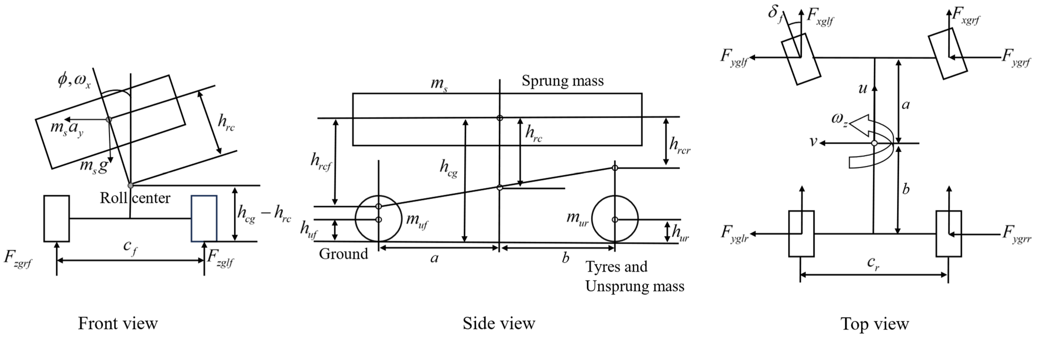
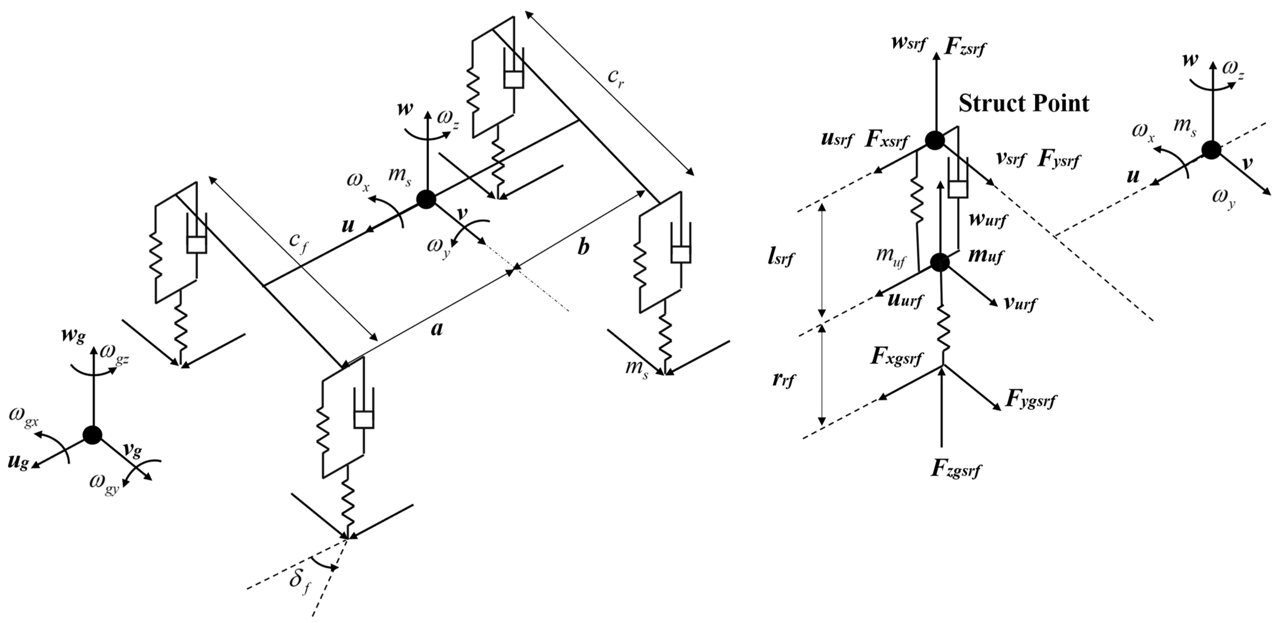
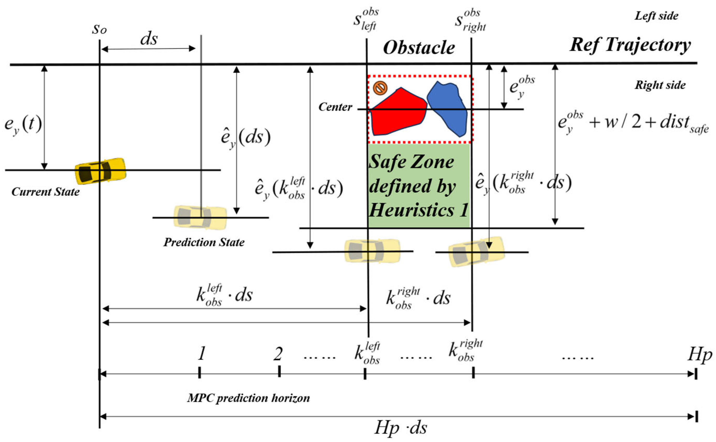
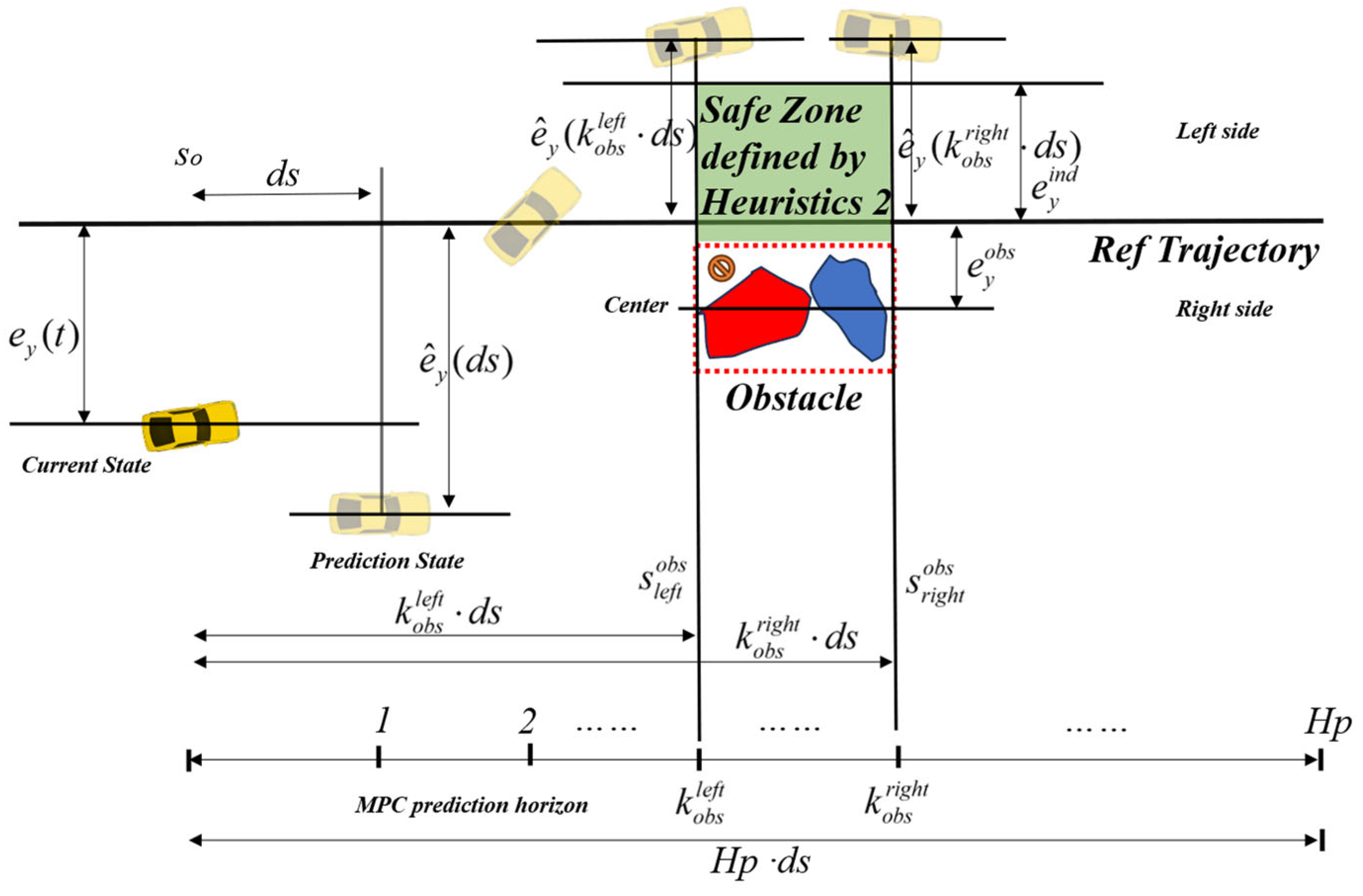
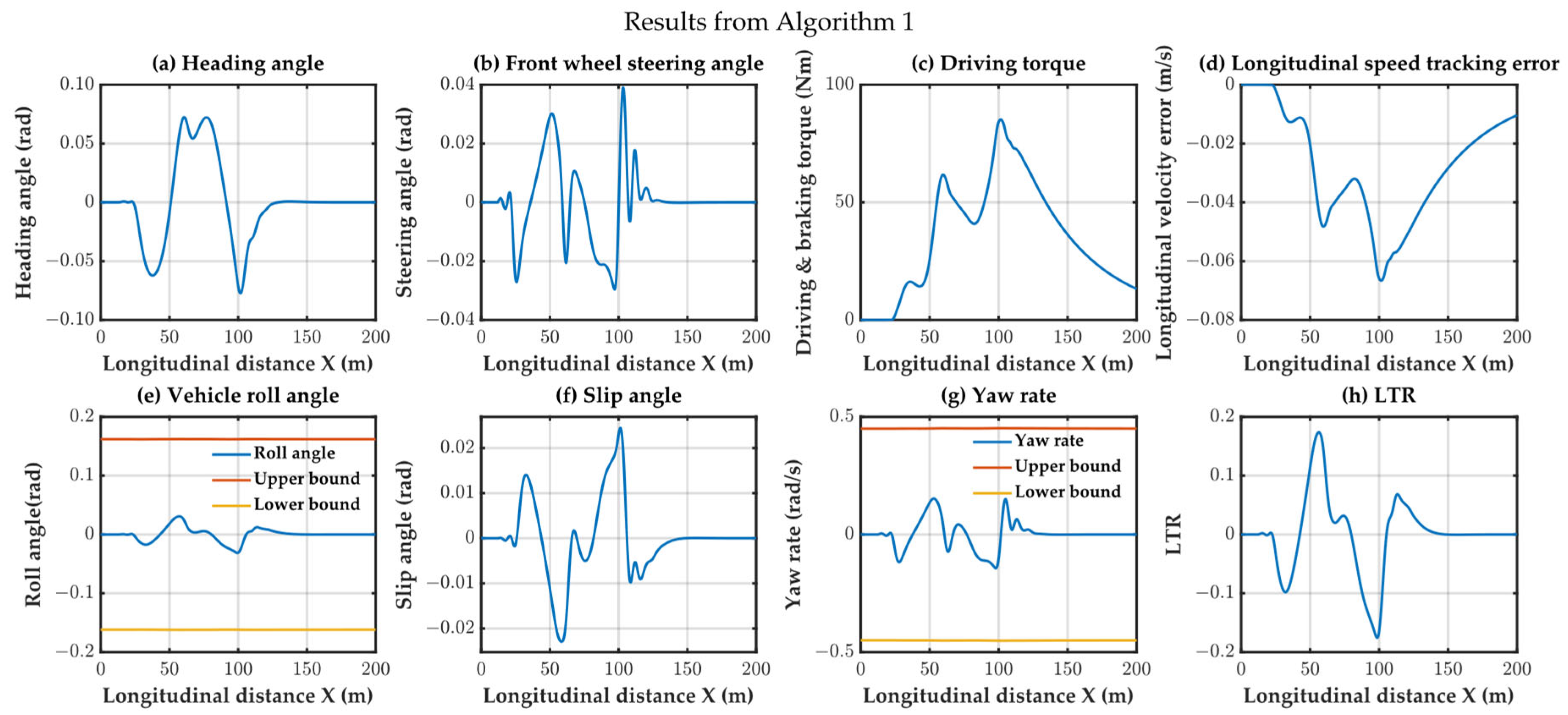
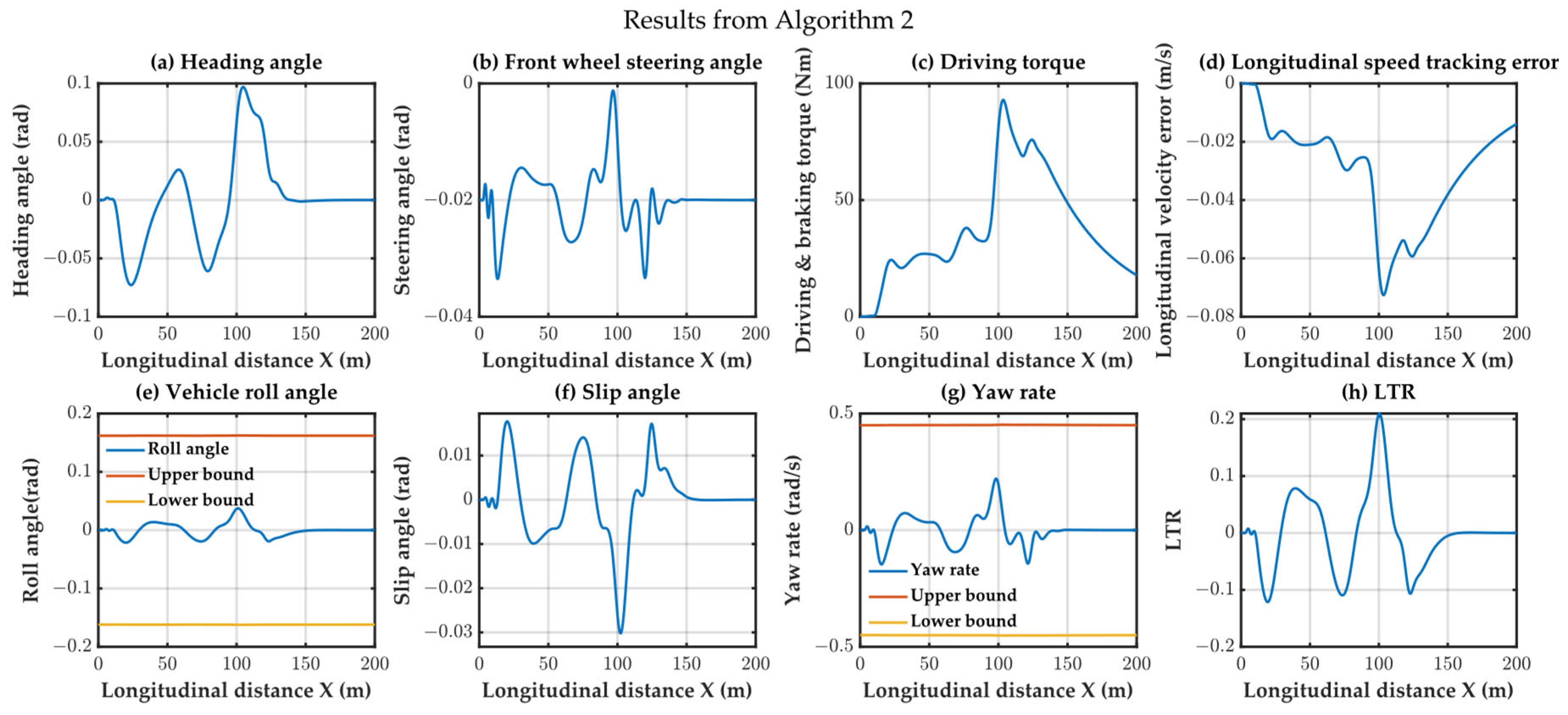
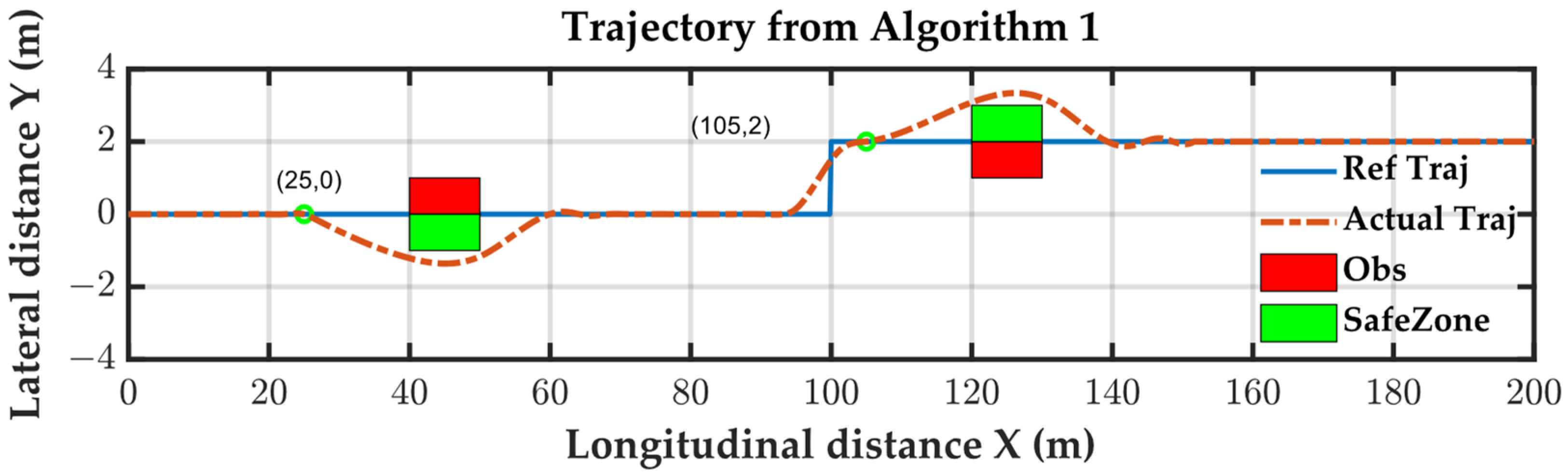
Table 1.
Simulation parameters.
| Parameter | Value |
|---|---|
| 1440 kg | |
| , , | 900 kg m2, 2000 kg m2, 2000 kg m2 |
| 1.15 m, 1.5 m | |
| 35,000 N/m, 32,000 N/m | |
| 0.75 m | |
| 1.5 m | |
| 2500 Ns/m, 2000 Ns/m | |
| 80 kg | |
| 30,000 N/m | |
| 0.285 m | |
| 0.65 m, 0.6 m | |
| 0.9 | |
| 30, 20 | |
| 0.5 m | |
| 0.05 s | |
| 1.5 | |
| (for upper-level MPC) | Diag([100, 100, 0, 0, 0, 0]) |
| (for upper-level MPC) | 200 |
| (for upper-level MPC) | 100 |
| (for lower-level MPC) | Diag([150, 120, 0, 0, 0, 0, 0, 0]) |
| (for lower-level MPC) | 150 |
Table 2.
Time consumption comparison of three algorithms in single-lane scenario.
| Algorithm 1 | Algorithm 2 | Algorithm 3 | ||||||
|---|---|---|---|---|---|---|---|---|
| Max | Mean | Median | Max | Mean | Median | Max | Mean | Median |
| 0.2000 | 0.1429 | 0.1430 | 0.2198 | 0.1548 | 0.1551 | 0.5420 | 0.4282 | 0.4343 |
Table 3.
Time consumption comparison of three algorithms in double-lane scenario.
| Algorithm 1 | Algorithm 2 | Algorithm 3 | ||||||
|---|---|---|---|---|---|---|---|---|
| Max | Mean | Median | Max | Mean | Median | Max | Mean | Median |
| 0.2713 | 0.1444 | 0.1443 | 0.2200 | 0.1513 | 0.1527 | 0.5403 | 0.4445 | 0.4395 |
Table 4.
Comparison of performance metrics between proposed algorithm and time-based MPC algorithms.
Table 4.
Comparison of performance metrics between proposed algorithm and time-based MPC algorithms.
| Predictability | Compatibility | Tracking Stability | Time Efficiency | |
|---|---|---|---|---|
| Algorithm 1 | ✓ | ✓ | ✓ | ✓ |
| Algorithm 2 | ✗ | ✗ | ✓ | ✓ |
| Algorithm 3 | ✗ | ✓ | ✗ | ✗ |
Disclaimer/Publisher’s Note: The statements, opinions and data contained in all publications are solely those of the individual author(s) and contributor(s) and not of MDPI and/or the editor(s). MDPI and/or the editor(s) disclaim responsibility for any injury to people or property resulting from any ideas, methods, instructions or products referred to in the content. |
© 2024 by the authors. Licensee MDPI, Basel, Switzerland. This article is an open access article distributed under the terms and conditions of the Creative Commons Attribution (CC BY) license (https://creativecommons.org/licenses/by/4.0/).
Share and Cite
MDPI and ACS Style
Yang, W.; Su, Y.; Chen, Y.; Lian, C. Integrated Spatial Kinematics–Dynamics Model Predictive Control for Collision-Free Autonomous Vehicle Tracking. Actuators 2024, 13, 153. https://doi.org/10.3390/act13040153
AMA Style
Yang W, Su Y, Chen Y, Lian C. Integrated Spatial Kinematics–Dynamics Model Predictive Control for Collision-Free Autonomous Vehicle Tracking. Actuators. 2024; 13(4):153. https://doi.org/10.3390/act13040153
Chicago/Turabian StyleYang, Weishan, Yixin Su, Yuepeng Chen, and Cheng Lian. 2024. "Integrated Spatial Kinematics–Dynamics Model Predictive Control for Collision-Free Autonomous Vehicle Tracking" Actuators 13, no. 4: 153. https://doi.org/10.3390/act13040153
Note that from the first issue of 2016, this journal uses article numbers instead of page numbers. See further details here.