Abstract
Bearing fault diagnosis is a pivotal aspect of monitoring rotating machinery. Recently, numerous deep learning models have been developed for intelligent bearing fault diagnosis. However, these models have typically been established based on two key assumptions: (1) that identical fault categories exist in both the training and testing datasets, and (2) the datasets used for testing and training are assumed to follow the same distribution. Nevertheless, these assumptions prove impractical and fail to accurately depict real-world scenarios, particularly those involving open-world assumption fault diagnosis in multi-condition scenarios. For that purpose, an open set domain adaptive adversarial network framework is proposed. Specifically, in order to improve the learning of distribution characteristics in different fields, comprehensive training is implemented using a deep convolutional autoencoder model. Additionally, to mitigate the negative transfer resulting from unknown fault samples in the target domain, the similarity of each target domain sample and the shared classes in the source domain are estimated using known class classifiers and extended classifiers. Similarity weight values are assigned to each target domain sample, and an unknown boundary is established in a weighted manner. This approach is employed to establish the alignment between the classes shared between the two domains, enabling the classification of known fault classes, while allowing the recognition of unknown fault classes in the target domain. The efficacy of our suggested approach is empirically validated using different datasets.
1. Introduction
The quality of bearings can directly impact the performance, reliability, and safety of rotating machinery. However, rolling bearings are susceptible to a variety of faults due to their frequent exposure to challenging conditions such as high loads and speeds. Moreover, bearing faults carry substantial maintenance costs and can have serious consequences, underscoring the critical importance of timely diagnosis and intervention. Early fault diagnosis methods have primarily relied on human expertise. However, such a manual approach is inadequate for the real-time diagnosis of bearing failure issues during operation.
With the rapid advancement in sensor and signal processing technologies, we can now extract robust features from collected data that aid in identifying the condition of bearings []. By employing deep learning models to discern the differences between normal operation and various fault states of bearings, we can accurately predict the presence of specific fault categories in an end-to-end manner. This approach effectively addresses the limitations of traditional fault diagnosis methods, which heavily rely on expert knowledge and manual intervention.
The current bearing fault diagnosis methods employ sophisticated deep learning models such as convolutional neural networks (CNN) [], autoencoders (AE) [], and graph convolutional neural networks (GCN) []. For example, Ince et al. [] employed a one-dimensional convolutional neural network model to directly analyze raw time-domain vibration signals to detect motor faults, thus significantly streamlining the time-consuming and labor-intensive feature extraction process. Mao et al. [] introduced a bearing fault diagnosis approach based on deep autoencoders, which effectively integrated multiple types of fault discrimination information. Their study demonstrated the method’s capability to extract deep features with enhanced representation, mitigate overfitting, and ensure model stability. Additionally, Cao et al. [] proposed an integrated transfer convolutional neural network that leveraged multi-sensor raw vibration signals, along with a newly devised decision fusion strategy, to classify fault types in gearboxes.
While significant progress has been made in utilizing mature deep learning models for intelligent bearing fault diagnosis, many current approaches are constrained by certain assumptions. Primarily, these methods assume that (1) the training and testing datasets share the same fault categories, and (2) the datasets used for testing and training adhere to the same distribution. However, in real-world industrial settings, bearing fault data can originate from diverse task requirements and environmental conditions. Consequently, the test dataset may include fault types not encountered in the training dataset, and there may be distributional disparities in the data collected under different operating conditions. Therefore, the aforementioned assumptions are impractical in practice.
To address the distributional differences in bearing fault data arising from various working conditions, many methods employ domain adaptation techniques. Domain adaptation can fully leverage the information from both the source and target domains to minimize the differences between distributions across different domains to the greatest extent possible. These approaches will be reviewed in detail in Section 2. However, the traditional domain adaptation methods have not effectively addressed the domain shift problem caused by the presence of unknown classes in the target domain. Therefore, a practical fault diagnosis model not only needs to align the distributions of shared categories of the two domains but also needs to have the ability to detect unknown classes, which is referred to as open set domain adaptation (OSDA) for fault diagnosis.
Research on the problem of OSDA is relatively mature in the field of computer vision. Busto and Gall [] first proposed the OSDA problem and used linear support vector machines to detect target anomalies. The open set domain adaptation by back-propagation (OSBP) method proposed by Saito et al. [] is an adversarial training strategy that constructs boundaries between known and unknown classes for classification purposes. In comparison, there is limited research in the literature on OSDA fault diagnosis, especially for rolling bearings.
Figure 1 shows the difference between closed-set and open set domain adaptation. To solve the OSDA bearing fault diagnosis problem, this study presents an open set domain adaptive adversarial network framework. First, we propose using a deep convolutional autoencoder model to better learn cross-domain fault category features. Then, we propose an adversarial model for domains. To encourage adversarial training and improve the positive transfer between samples, this paper assigns weights to target samples based on a similarity analysis between the target domain samples and known classes. In the test phase, the input sample’s category is determined by the unknown class classifier. The following are this paper’s main contributions:
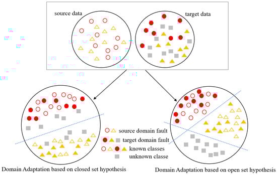
Figure 1.
The difference between closed sets and open sets in domain adaptation.
(1) To address diverse domains or data distributions, we integrate supervised multiple classifiers with unsupervised deep convolutional autoencoders to accomplish known fault classification and capture intricate data distributions. The feature distributions of the samples in the target and source domains are successfully aligned by improving the encoder and decoder and using the scale-invariant mean squared error, leading to improved performance in bearing fault diagnosis.
(2) To address negative transfer in open set fault diagnosis, we employ multiple classifiers to compute similarity weights for target domain samples, learning their likelihood of belonging to shared categories. These weights are incorporated into the corresponding target domain samples, thereby excluding the unknown fault samples from the target domain and mitigating domain classification loss error.
(3) We conducted experiments on three laboratory bearing datasets, evaluating different transfer fault tasks and conducting a comparative analysis. Our findings emphatically demonstrated the effectiveness of our proposed open set domain adaptation method.
The remainder of this paper is structured as follows: Section 2 introduces the development of existing related work in domain adaptation. Section 3 elaborates on the design of the proposed OSDA method. Section 4 describes the experimental settings on multiple datasets and presents the validation and analysis of the experimental results. Finally, Section 5. provides a summary of the key findings and conclusions of this study.
2. Related Work
We briefly introduce various recent domain adaptation methods. These methods primarily address the constraint of label set relationships between different domains and are categorized into closed domain adaptation, partial domain adaptation, and open domain adaptation.
(a) Closed-Set Domain Adaptation (CSDA). As mentioned, CSDA means sharing the same class in both the source and target domains, focusing primarily on the goal of mitigating the performance degradation caused by domain differences. Early feature adaptation methods mainly relied on traditional statistical learning techniques to map or transform features from the source domain to the target domain, such as PCA, LDA, etc. As deep learning research has advanced, statistical moment alignment has become a popular approach. For example, Tzeng et al. [] first used the maximum mean discrepancy (MMD) distance to measure the distance between two domains, achieving as much as possible alignment between domains. Long et al. [] proposed a deep adaptation network (DAN) structure that extends deep convolutional neural networks to domain adaptation scenarios. Compared to MMD’s use of a single kernel function, DAN is extended to multiple kernels and linear combinations of kernel functions, achieving minimization of the maximum average difference between deep feature cross-domain distributions. Taking into account that target and source domains are not fully consistent, Long et al. [] improved DAN by introducing residual transfer network structures into the source domain classifier and adding an entropy minimization criterion in the target domain. To further learn the differences in labels by considering domain differences, Long et al. [] generalized the kernel function to a joint distribution through inner product operations.
With the emergence of generative adversarial networks (GANs), there has been a gradual increase in research focusing on adversarial learning applied to domain adaptation. This approach involves training a domain classifier, also called a discriminator, to distinguish between source and target domain features, while simultaneously training the feature extractor to confuse this discriminator by generating domain-invariant features []. Goodfellow et al. [] proposed a generative framework based on adversarial learning, which trained models through competition. Ganin et al. [] used a domain discriminator to distinguish two domains, and in the domain adversarial training paradigm, the feature extractor learned to confuse the domain discriminator.A conditional domain adversarial network(CDAN) [] was also introduced to improve the domain adversarial network by matching the joint distribution of labels and features. The aforementioned work laid the foundation for further development of the field.
(b) Partial Domain Adaptation (PDA). Compared with traditional closed-set domain adaptation methods, partial domain adaptation assumes that the label spaces between the source and target domains are not completely identical and that the label set of the source domain should be large enough to include the target label set [], which is more suitable for applications in big data scenarios. In order to solve the problem of partial domain adaptation in bearing fault diagnosis, many researchers have used a weighting method to distinguish between private and shared labels. Kuang et al. [] proposed a double weighting method to align the weighted data by combining the class weights obtained by the classifier and the sample weights obtained by the domain discriminator. Wang et al. [] incorporated class level weights into a DANN model and employed a balancing strategy to augment classes in the target domain with source samples to expand classes in the target domain using source samples to alleviate the negative impact of label space asymmetry. Huang et al. [] added pseudo labels to the target domain samples and then used them to selectively weight the source features. Based on the introduction of the above methods, most PDA methods add weight to the source domain samples and filter out the data that only exists in the source domain label space.
(c) Open Set Domain Adaptation (OSDA). As mentioned, OSDA refers to the case that the source domain label set is a subset of the target domain label set. It assumes that the label set of the target domain is larger than the label set of the source domain, where the private class samples contained in the target domain are called unknown classes. The goal is to achieve accurate classification of known class samples in the target domain, while labeling private samples as unknown classes. Busto et al. [] first proposed OSDA, which uses the assign and transform iteratively (ATI) algorithm to map the target samples to source classes and then trains an SVM for final classification. However, the ATI algorithm assumes the presence of unknown classes in the source domain that are not present in the target domain. The OSBP [] method introduced by Saito et al. mitigates such assumptions. It employs a domain adversarial approach, emphasizing the establishment of an unknown boundary on the unknown class samples in the target domain using a fixed threshold. Furthermore, it extends the classifier by incorporating an additional unknown class discriminator. Liu et al. [] carried out further investigation on the basis of the OSBP method, incorporating a coarse-to-fine weighted mechanism to gradually separate unknown and known samples, while balancing their importance for feature distribution alignment.
However, research on adaptive open set learning in the field of fault diagnosis is still limited. Currently, the majority of the existing methods rely on weighted approaches. For instance, Zhang et al. [] introduced adversarial learning to extract generalized features and implemented an instance-level weighting mechanism to estimate the similarity between target and source domain samples, which was combined with entropy minimization to further improve the model’s generalization ability. Zhao et al. [] studied a method based on dual adversarial learning. The weights assigned to the target samples by the auxiliary domain discriminator effectively distinguished the unknown classes. Guo et al. [] achieved open set MMC fault diagnosis and distinguished known and unknown faults by introducing techniques such as batch normalization and layer normalization and by designing a multi-scale coordinate residual attention mechanism. Zhu et al. [] realized domain adaptation and feature selective distribution alignment in open set intelligent bearing fault diagnosis through a weight transfer conditional countermeasure network and weighted countermeasure learning network. These methods can effectively identify unknown fault categories and improve the recognition rate of known categories. In this paper, our approach builds on the aforementioned OSDA methods and incorporates a novel multi-classifier module with a novel weighting scheme to automatically establish boundaries between known and unknown target samples, achieving their alignment.
3. Method
3.1. Problem Definition
The domain adaptation problem is formally defined using the open set hypothesis. Let the training data be labeled samples from the dataset , which fits with the distribution of source domain and the label space . The test data should similarly include unlabeled samples from the target domain distribution and the label space , which correspond to the dataset , where and . The shared classes are defined by the intersection of and , and the private labels in the target domain should be regarded as “unknown”.
In order to accomplish cross-domain alignment of shared categories and discover unknown fault categories in the target domain, an open set domain adaptive adversarial network model has to be established.
3.2. Open Set Adversarial Domain Adaptation Framework
The method proposed in this paper, along with its deep neural network architecture consists of four key modules, as shown in Figure 2. These modules, denoted as , , , and , serve as a feature extractor, a known-class classifier, and an extended classifier, respectively. The feature extractor incorporates deep convolutional autoencoders ( and ) to autonomously learn enriched and refined representations from raw inputs of both domains. To mitigate the classification loss emanating from the source domain, a known-class classifier is used. It outputs the probability value for the K-th dimension. Furthermore, an extended classifier , encompassing both known and unknown categories, is introduced. Compared with the known-class classifier , the dimension of the output from increases from K to , where the dimension outputs the similarity weight that shows whether the sample is an unknown class.Detailed parameters of the model are shown in Table 1.
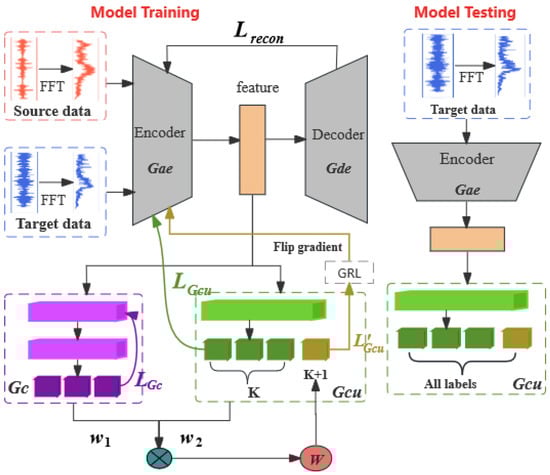
Figure 2.
An Open Set Domain Adaptation Model Framework Based on Adversarial Learning.

Table 1.
Detailed parameters of the model.
3.3. Deep Autoencoders and Reconstruction Error
The studies in [,] indicated that autoencoders can serve as substitutes for neural network structures in discrimination tasks. Motivated by this, we introduce a deep convolutional autoencoder as a replacement for a convolutional neural network in the context of adversarial learning for domain adaptation, thereby enhancing feature learning. It consists of two components, an encoder and a decoder . projects the input bearing data into an encoding space while preserving crucial characteristics of the bearing signals. re-projects the encoded data in the latent space back to the input space, generating reconstructed bearing data for comparison with the original data, to minimize reconstruction error loss.
The deep convolutional autoencoder utilizes unsupervised learning to reconstruct data, aiming to encapsulate the data distributions of both domains. This strategy uncovers intrinsic feature variations and pursues a common latent distribution. The optimization process is geared towards making the reconstructed data closely resemble the original input by fine-tuning the model parameters through a defined loss function.
For the calculation of the reconstruction loss, we employ a scale-invariant mean squared error term [], which is applied to data from both the target and source domains.
Here, k represents the dimension of the sample data, represents the reconstructed data from the model, and refers to the L2 squared norm. It is important to note that predictions that are accurate up to a scaling term are penalized by the mean squared error (MSE) loss, which is commonly used in reconstruction tasks. In contrast, the scale-invariant mean squared error penalizes discrepancies between frequency components, enabling the model to replicate the general shape of the represented object more effectively, thereby reducing reconstruction errors and approximating the original input data as closely as possible.
3.4. Target Domain Sample Weight Calculation
Training the model on the source domain is a crucial step to enable the classification of known faults. In this paper, to learn the feature distribution of source domain samples, we train the extended classifier in a supervised manner using conventional cross-entropy loss to optimize the classification of source domain data.
Here, and represent the parameters of the and the , and symbolizes the quantity of samples in the source domain. The common cross-entropy loss function used to reduce the error is denoted by . and represent the labels corresponding to the samples in the source domain .
Since the learning parameters of the known class classifier are only trained on source samples, target samples with distributions differing from the source will have lower similarity values or uncertain predictions. The classifier utilizes a multiclass one-vs-rest binary loss to compute the loss. The formula is as follows:
where represents the one-hot encoded label of the source domain sample.
To reduce the risks of misclassifying unknown fault categories in the target domain as known categories, we have devised a weighting method for the input sample which is based on its similarity to the source domain’s known shared labels. As shown in Equation (4) below, calculates the sum of the k-dimensional probabilities for the known class, leveraging to utilize the label information from the known classes in the source domain. This approach effectively minimizes the influence of samples from unknown classes in the target domain, while aligning the samples of known classes between the two domains.
where represents the probability that the sample belongs to the Kth known category, and the sum represents the similarity weight between the target sample and the known class in the source domain. For target domain samples similar to the source domain samples, the softmax element output and will be elevated or nearly one, while samples that are different from the source domain will have an output close to zero. Hence, we can utilize the output values of to quantify the transferability of samples between the target and source domains.
However, since the definition of this similarity measure is trained only on the source domain class labels, the values for target samples may be uncertain. Therefore, it is necessary to further understand the intrinsic characteristics of target domain samples.
We investigate the distribution changes of unknown class samples in the target domain based on the similarity measure of known class samples labeled in the source domain. This is done through the utilization of the -th dimensional unknown class probability within the extended classifier , thereby quantifying the similarity weight for target samples that are part of the shared space.
When the target sample is a member of the shared label set, the value of is relatively low, thus requiring a higher weight to be assigned to this sample. This is represented by Equation (5).
In the domain adversarial model, the similarity between known and target K class samples from the source domain is determined using the known class classifier . For target domain samples, their affiliation with shared categories is determined based on the unknown class decisions made by the extended classifier . Ultimately, by analyzing the foundational domain information, weights are assigned to target domain samples. The final similarity measure is then defined by combining the outputs of the known class classifier and the extended classifier .
By combining the similarity weights of and , the similarity weight values assigned to each sample in the target domain are measured. is regarded as a comprehensive measure of the possibility that the target domain sample belongs to the shared label space. To further validate this conclusion, Section 4.3 provides visual evidence of this theory through the display of target domain sample weights.
However, in open set domain adaptation problems, if the private label data of the target domain are ignored, this could lead to erroneous matching of unknown class samples in the target domain with labeled samples in the source domain, resulting in negative transfer issues during cross-domain alignment.
To address this issue, similarity weight values, , are computed using multiple classifiers to calculate the similarity between samples from the source and target domains. These similarity weights are then added to each corresponding target domain sample, reducing the domain classification loss error and thereby avoiding negative transfer issues.
3.5. Establishment of Unknown Boundary
To better align known classes in the target domain with the source domain, while keeping unknown classes away from the source domain, we employ binary cross-entropy loss in Equation (7) to learn an accurate hyperplane. The bounds of the target domain’s unknown class samples are defined by this hyperplane.
Unlike the approach used in OSBP [], which sets a boundary threshold T to distinguish between shared labels and private labels for constructing an unknown class boundary, this study replaces the fixed threshold for target domain samples with dynamic similarity weights . This is represented as follows:
Based on the aforementioned derivations, we introduce the adversarial domain adaptation model. The following is an overview of this approach’s main goals:
The above equation reflects the minimax game between the deep autoencoder and the extended classifier . It adversarially fools the extended classifier through the deep autoencoder and reduces the difference between the source domain and the target domain by learning transferable features.
Based on the characteristics of binary cross-entropy, the extended classifier attempts to set an unknown class probability equal to , thus minimizing the value of . Conversely, the deep autoencoder strives to make different from , in order to maximize the value of . The extended classifier ’s unknown class probability can be changed by the deep autoencoder during training. When the weight is relatively high, the sample aligns with the known categories, and as a result, the value of should be lower. However, the extended classifier attempts to minimize by increasing the value of to match the weight , which in turn leads to the sample moving away from the source domain. Conversely, the objective of the deep autoencoder is to maximize , which leads to an increase in the distance between and . Consequently, this decreases the value of , bringing the sample closer to those in the source domain. This configuration results in an adversarial relationship between them. Through such adversarial training, attempts to confuse the target domain’s shared and unknown classes, making them difficult to distinguish. Meanwhile, strives to generate distinctive features that facilitate separating known classes from unknown ones in the target samples.
All training loss functions are optimized using an end-to-end approach [] and reversing the gradient sign during backpropagation. Ultimately, the open set domain adaptive problem is well handled, whereby the unknown samples in the target domain can be accurately identified, reducing the cross-domain differences and promoting positive migration. The pseudocode for this method is provided in Algorithm 1.
| Algorithm 1: Proposed Methodology |
Input: Source domain data , target domain data , and source domain labels , initialize network parameters, number of epochs: N, number of batch size: B. Output: the target domain sample label . 1. For epoch=1 to N do 2. For i=1 to B do 3. Feed the source and target dataset into feature extractor to obtain common features: , . 4. Feed the common features of the source and target dataset into known-class classifier and extended classifier simultaneously. 5. For , compute the multiclass one-vs-rest binary loss for the source domain with (3) and similarity measure with (4). 6. For , compute the cross entropy with (2) and similarity measure with (5). 7. Compute the final similarity measure with (6). 8. Calculate the loss of with (7). Backpropagation: Using stochastic gradient descent method to optimize the parameters of the model from (8) to (10) 9. End 10. End |
4. Experimental Results and Discussion
4.1. Dataset Description
To verify the effectiveness of our proposed method, we conducted extensive evaluation experiments using three different types of bearing datasets namely, the Case Western Reserve University (CWRU) dataset, the Southeast University (SEU) dataset, and the Padburn (PU) dataset. For the three datasets used in this paper, a vibration signal of length 4098 was first selected from the raw signal, and 4098 Fourier coefficients were produced by performing an FFT. Since the coefficients were symmetric, only 2049 coefficients were considered. The different tasks set by these datasets have specific labels and interpretations, and the details are shown in Table 2, Table 3, Table 4 and Table 5.
Table 2.
CWRU information and particular job settings.
Table 3.
SEU information and particular job settings.
Table 4.
PU dataset working condition information.
Table 5.
PU information and particular job settings.
CWRU Bearing Dataset: There were four distinct circumstances represented in the vibration signals obtained from the motor’s driving end on the test rig: (1) healthy state (H); (2) inner-race fault (IF); (3) outer-race fault (OF); and (4) ball fault (BF).There were three distinct severity levels for the IF, OF, and BF cases (0.007 inches, 0.014 inches, and 0.021 inches) corresponding to the vibration signals. The sampling frequency was 12 kHz, and the signals were collected under four different working conditions of motor load and speed: load 0, load 1, load 2, and load 3 respectively. More details of the CWRU bearing data can be viewed from []. The configuration of the CWRU dataset is shown in Table 2.
SEU Bearing Dataset: This dataset is provided by Southeast University. The dataset contents and further details can be found in []. The gear dataset and the bearing dataset are two of its sub-datasets. Vibration signals were collected at 12 kHz under two different operating conditions with the velocity load configuration (RS-LC, respectively) set to 20 Hz-0 V and 30 Hz-2 V. Under each operating condition, the bearing had four states: H, IF, OF, and BF. There are eight lines of vibration signals in each file, but only the second line was included in this study.
PU Bearing Dataset: The PU dataset [] is provided by the University of Padbourne and consists of 32 sets of current signals and vibration signals. The bearing signals are categorized as follows: (1) 6 undamaged bearings; (2) 12 artificially damaged bearings; and (3) 14 bearings that were actually damaged due to accelerated life testing. In this section, the main bearing signals used were from the undamaged healthy state (H) and artificially damaged bearings, which included outer race faults (IF) and inner race faults (OF). Therefore, the dataset included three fault types: H, IF, and OF. Each dataset was collected in four distinct operating situations at a sampling frequency of 64 kHz. Table 4 provides a detailed overview of the distribution, while the specific experimental settings are presented in Table 5.
4.2. Experimental Result Analysis
The test accuracy of our method on the different open set domain adaptation tasks from the different datasets is presented in Table 6. In this table, the target domain classification accuracy for shared classes is denoted by K, recognition accuracy for unknown classes is represented by U, and total accuracy is denoted by .
Table 6.
Novelty detection performance of CWdatasets.
As demonstrated, the low results for unknown class recognition in task C5 were an exception. In the other tasks, both the recognition accuracy for unknown classes and the categorization accuracy for known classes surpassed 96.7%, indicating a high testing accuracy. While the CWRU dataset exhibited a simpler distribution compared to the SEU and PU datasets, the overall experimental results of the latter two datasets also achieved over 90% accuracy, except for the individual tasks. Overall, the experimental findings across all three datasets affirmed that our proposed method, when employed within the open set domain adaptation framework, could achieve accurate classification of known class data and had robust recognition capability for unknown class data.
4.3. Feature Visualization Result Analysis
To visually validate the performance of the proposed approach in domain adaptation under the open set assumption, we utilized t-SNE visualization. Here, U represents unknown fault samples. We obtained the t-SNE visualization results shown in (a), (b), and (c) of Figure 3, Figure 4 and Figure 5 by transforming the time-domain data into frequency-domain data using the FFT method. Additionally, the t-SNE visualization results shown in (d), (e), and (f) of Figure 3, Figure 4 and Figure 5 represent the high-level features learned by the feature extractor module from the source and target domain data. Three representative sets were selected from each dataset for visualization. These results demonstrated the visualization comparison before and after domain adaptation based on the open set assumption for tasks C0, C4, and C8 from the CWRU dataset; S0, S3, and S5 from the SEU dataset; and P0, P1, and P3 from the PU dataset in the source and target domains.
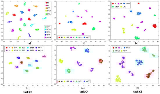
Figure 3.
Visualization results of different tasks in CWRU dataset before and after domain adaptation. (a–c) represent the effect of data after FFT. (d–f) denote the effect of data adaptive by the method in this paper.
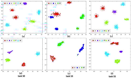
Figure 4.
Visualization results of different tasks in SEU dataset before and after domain adaptation. (a–c) represent the effect of data after FFT. (d–f) denote the effect of data adaptive by the method in this paper.
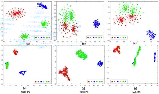
Figure 5.
Visualization results of different tasks in PU dataset before and after domain adaptation. (a–c) represent the effect of data after FFT. (d–f) denote the effect of data adaptive by the method in this paper.
Taking the C0 task from the CWRU dataset as a detailed example. The visualization results from Figure 3a revealed that before domain adaptation alignment, the shared class samples across the source and target domains were dispersed and clearly did not belong to the same fault category. However, following domain adaptive alignment, as depicted in Figure 3d, the shared class samples across the source and target domains became closer together and fell under the same classification. Meanwhile, the unknown categories were excluded, indicating alignment between the cross-domain samples and enabling the identification of unknown fault samples in the target domain. This illustrates an effective enhancement in cross-domain diagnostic performance under source supervision.
Similar visualization results based on the open set assumption could be observed in the other tasks as well. These visualization results demonstrated that the methodological framework of this paper could align class-level features across domains. It effectively projected the shared health states in the target and source domain samples to the same region in the high-level representation space and isolated the anomaly categories of the target domain in separate regions.
This suggests that our proposed approach could successfully learn the information from the source domain and apply it to the target domain, and it could also accurately identify unknown target categories to prevent negative transfer.
We also depict the weights learned from the known and undiscovered fault categories in the target domain for the various datasets to further support the efficacy of our suggested weight-based technique. Figure 6 illustrates the corresponding weight values of target domain samples for tasks C0, C4, and C8 in the CWRU dataset. Figure 7 shows the corresponding weight values of target domain samples for tasks S0, S3, and S5 in the SEU dataset, and Figure 8 shows the corresponding weight values of target domain samples for tasks P0, P1, and P3 in the PU dataset. If the samples between the target and source domains have the same health status labels, they will have a higher weight. On the other hand, for target outlying classes, i.e., unknown fault classes, lower weights are assigned. For example, for Task C8, the target domain labels included normal bearings (H), outer race faults with 0.007 inches diameter damage (OF7), outer race faults with 0.014 inches diameter damage (OF14), and outer race faults with 0.021 inches diameter damage (OF21). The weights learned by the corresponding samples fluctuated above 0.4, indicating that they had obtained high-level weight values, thus had high similarity with the source domain’s fault categories, and were more focused on the learning process of domain adaptive alignment of shared category samples. The learned weights roughly fluctuated below 0.2, with low weight values for unknown fault samples (U) in the target domain. They did not correspond with shared category samples and were therefore less frequently taken into account in the cross-domain distributions. The target domain samples’ weight visualization findings demonstrated comparable learning in other tasks. The visualization of the weight maps verified the effectiveness of similarity weights, which combine known and unknown classes, as a weighting method in our proposed domain adaptive process of bearing fault diagnosis.
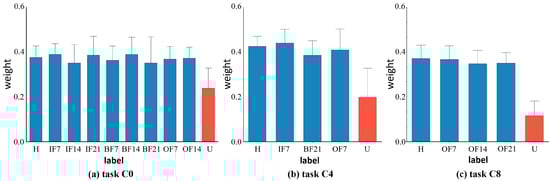
Figure 6.
The average value and deviation of the corresponding weight of each fault type of the target sample under different tasks of the CWRU dataset. Red indicates unknown class and blue indicates known class.
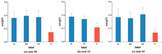
Figure 7.
The average value and deviation of the corresponding weight of each fault type of the target sample under different tasks of the SEU dataset. Red indicates unknown class and blue indicates known class.
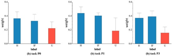
Figure 8.
The average value and deviation of the corresponding weight of each fault type of the target sample under different tasks of the PU dataset. Red indicates unknown class and blue indicates known class.
4.4. Experimental Comparisons
We also conducted comparative experiments using different task settings of the CWRU, SEU, and PU datasets against other classical methods such as DANN [], CORAL [], OSBP [], improved OSBP [], and STA []. The results are shown in Figure 9, Figure 10 and Figure 11, comparing the comprehensive performance of the representative domain adversarial methods and the proposed method. In summary, our proposed strategy outperformed the competing methods in the related tasks.
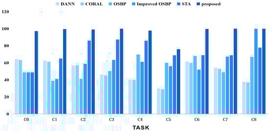
Figure 9.
Accuracy tests using various techniques on the CWRU dataset for open set domain adaption tasks.
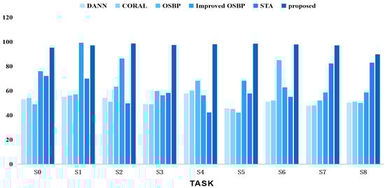
Figure 10.
Accuracy tests using various techniques on the SEU dataset for open set domain adaption tasks.
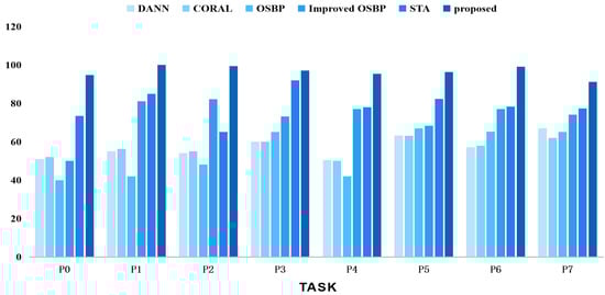
Figure 11.
Accuracy tests using various techniques on the PU dataset for open set domain adaption tasks.
4.5. Future Work
In practical applications, partial domain adaptation is also common and useful, where the source domain categories are more numerous than the target domain categories. To better adapt to various scenarios, there is an urgent need to establish a more generalized and unified domain adaptation framework suitable for different working conditions.
The methodology of this paper investigated single-source domain adaptation, where the similarity between the source and target domains is usually high, leading to significant achievements in cross-domain diagnosis. However, real-world fault diagnosis scenarios face substantial variations in machine operating conditions, resulting in significant differences between the two domains under different working conditions. Relying on single source domain data may not be sufficient for accurate diagnosis under diverse working conditions. In industrial settings, we often have access to labeled data from multiple operating conditions. Therefore, leveraging diagnostic knowledge from various working conditions can better address fault diagnosis challenges in extreme working conditions. This approach involving multiple working conditions provides a more comprehensive and flexible adaptability, promising to enhance the robustness of the model in practical industrial applications.
5. Conclusions
In the existing application field of mechanical industry, the open world hypothesis is an unavoidable real-world approach to accurately classifying and identifying bearing faults under different working conditions and fault labels.The two aforementioned problems were addressed by this study’s investigation of an open-world domain adaptive intelligent fault detection approach for rolling bearings. We introduced a domain adversarial model to construct the network architecture and employed a deep convolutional autoencoder to extract domain-invariant features. We successfully aligned the target and source domains, while limiting the influence of unknown classes by using the similarity between target domain samples and known classes to contribute shared weights to the discriminator. The suggested approach was the subject of numerous sets of experiments, and its validity was thoroughly examined.
Author Contributions
Data curation, B.Z., F.L. and N.M.; methodology, B.Z., F.L. and W.J.; software B.Z. and F.L.; formal analysis, N.M., W.J. and S.-K.N.; writing—original draft, B.Z. and F.L.; writing—review and editing, B.Z., F.L., W.J. and S.-K.N. All authors have read and agreed to the published version of the manuscript.
Funding
This work was supported by “the Fundamental Research Funds for the Central Universities” 2019ZDPY08. (Corresponding author: Wen Ji).
Institutional Review Board Statement
Not applicable.
Informed Consent Statement
Not applicable.
Data Availability Statement
Data are contained within the article.
Conflicts of Interest
The authors declare no conflicts of interest.
References
- Cao, H.; Shao, H.; Zhong, X.; Deng, Q.; Yang, X.; Xuan, J. Unsupervised domain-share CNN for machine fault transfer diagnosis from steady speeds to time-varying speeds. J. Manuf. Syst. 2022, 62, 186–198. [Google Scholar] [CrossRef]
- Wen, L.; Li, X.; Gao, L.; Zhang, Y. A new convolutional neural network-based data-driven fault diagnosis method. IEEE Trans. Ind. Electron. 2017, 65, 5990–5998. [Google Scholar] [CrossRef]
- Sohaib, M.; Kim, J.M. Reliable fault diagnosis of rotary machine bearings using a stacked sparse autoencoder-based deep neural network. Shock Vib. 2018, 2018, 2919637. [Google Scholar] [CrossRef]
- Li, T.; Zhao, Z.; Sun, C.; Yan, R.; Chen, X. Multireceptive field graph convolutional networks for machine fault diagnosis. IEEE Trans. Ind. Electron. 2020, 68, 12739–12749. [Google Scholar] [CrossRef]
- Ince, T.; Kiranyaz, S.; Eren, L.; Askar, M.; Gabbouj, M. Real-time motor fault detection by 1-D convolutional neural networks. IEEE Trans. Ind. Electron. 2016, 63, 7067–7075. [Google Scholar] [CrossRef]
- Mao, W.; Feng, W.; Liu, Y.; Zhang, D.; Liang, X. A new deep auto-encoder method with fusing discriminant information for bearing fault diagnosis. Mech. Syst. Signal Process. 2021, 150, 107233. [Google Scholar] [CrossRef]
- He, Z.; Shao, H.; Zhong, X.; Zhao, X. Ensemble transfer CNNs driven by multi-channel signals for fault diagnosis of rotating machinery cross working conditions. Knowl.-Based Syst. 2020, 207, 106396. [Google Scholar] [CrossRef]
- Panareda Busto, P.; Gall, J. Open set domain adaptation. In Proceedings of the IEEE International Conference on Computer Vision, Venice, Italy, 22–29 October 2017; pp. 754–763. [Google Scholar]
- Saito, K.; Yamamoto, S.; Ushiku, Y.; Harada, T. Open set domain adaptation by backpropagation. In Proceedings of the European Conference on Computer Vision (ECCV), Munich, Germany, 8–14 September 2018; pp. 153–168. [Google Scholar]
- Tzeng, E.; Hoffman, J.; Zhang, N.; Saenko, K.; Darrell, T. Deep domain confusion: Maximizing for domain invariance. arXiv 2014, arXiv:1412.3474. [Google Scholar]
- Long, M.; Cao, Y.; Wang, J.; Jordan, M. Learning transferable features with deep adaptation networks. In Proceedings of the International Conference on Machine Learning, Lille, France, 7–9 July 2015; pp. 97–105. [Google Scholar]
- Long, M.; Zhu, H.; Wang, J.; Jordan, M.I. Unsupervised domain adaptation with residual transfer networks. Adv. Neural Inf. Process. Syst. 2016, 29. [Google Scholar] [CrossRef]
- Long, M.; Zhu, H.; Wang, J.; Jordan, M. Deep transfer learning with joint adaptation networks. In Proceedings of the International Conference on Machine Learning, Sydney, Australia, 6–11 August 2017; pp. 2208–2217. [Google Scholar]
- Tzeng, E.; Hoffman, J.; Saenko, K.; Darrell, T. Adversarial discriminative domain adaptation. In Proceedings of the IEEE Conference on Computer Vision and Pattern Recognition, Honolulu, HI, USA, 21–26 July 2017; pp. 7167–7176. [Google Scholar]
- Goodfellow, I.; Pouget-Abadie, J.; Mirza, M.; Xu, B.; Warde-Farley, D.; Ozair, S.; Courville, A.; Bengio, Y. Generative adversarial networks. Commun. ACM 2020, 63, 139–144. [Google Scholar] [CrossRef]
- Ganin, Y.; Ustinova, E.; Ajakan, H.; Germain, P.; Larochelle, H.; Laviolette, F.; Marchand, M.; Lempitsky, V. Domain-adversarial training of neural networks. J. Mach. Learn. Res. 2016, 17, 2030–2096. [Google Scholar]
- Long, M.; Cao, Z.; Wang, J.; Jordan, M.I. Conditional adversarial domain adaptation. Adv. Neural Inf. Process. Syst. 2018, 31. [Google Scholar] [CrossRef]
- Cao, Z.; Long, M.; Wang, J.; Jordan, M.I. Partial transfer learning with selective adversarial networks. In Proceedings of the IEEE Conference on Computer Vision and Pattern Recognition, Salt Lake City, UT, USA, 18–23 June 2018; pp. 2724–2732. [Google Scholar]
- Kuang, J.; Xu, G.; Tao, T.; Wu, Q.; Han, C.; Wei, F. Dual-weight consistency-induced partial domain adaptation network for intelligent fault diagnosis of machinery. IEEE Trans. Instrum. Meas. 2022, 71, 1–12. [Google Scholar] [CrossRef]
- Wang, Y.; Liu, Y.; Chow, T.W.; Gu, J.; Zhang, M. A Balanced Adversarial Domain Adaptation Method for Partial Transfer Intelligent Fault Diagnosis. IEEE Trans. Instrum. Meas. 2022, 71, 1–11. [Google Scholar] [CrossRef]
- Huang, Q.; Wen, R.; Han, Y.; Li, C.; Zhang, Y. Intelligent Fault Identification for Industrial Internet of Things via Prototype Guided Partial Domain Adaptation with Momentum Weight. IEEE Internet Things J. 2023, 10, 16381–16391. [Google Scholar] [CrossRef]
- Liu, H.; Cao, Z.; Long, M.; Wang, J.; Yang, Q. Separate to adapt: Open set domain adaptation via progressive separation. In Proceedings of the IEEE/CVF Conference on Computer Vision and Pattern Recognition, Long Beach, CA, USA, 15–20 June 2019; pp. 2927–2936. [Google Scholar]
- Zhang, W.; Li, X.; Ma, H.; Luo, Z.; Li, X. Open-set domain adaptation in machinery fault diagnostics using instance-level weighted adversarial learning. IEEE Trans. Ind. Inform. 2021, 17, 7445–7455. [Google Scholar] [CrossRef]
- Zhao, C.; Shen, W. Dual adversarial network for cross-domain open set fault diagnosis. Reliab. Eng. Syst. Saf. 2022, 221, 108358. [Google Scholar] [CrossRef]
- Guo, Q.; Li, J.; Zhou, F.; Li, G.; Lin, J. An open-set fault diagnosis framework for MMCs based on optimized temporal convolutional network. Appl. Soft Comput. 2023, 133, 109959. [Google Scholar] [CrossRef]
- Zhu, Z.; Chen, G.; Tang, G. Domain Adaptation with Multi-adversarial Learning for Open Set Cross-domain Intelligent Bearing Fault Diagnosis. IEEE Trans. Instrum. Meas. 2023, 72, 3533411. [Google Scholar] [CrossRef]
- Zhao, J.; Mathieu, M.; LeCun, Y. Energy-based generative adversarial network. arXiv 2016, arXiv:1609.03126. [Google Scholar]
- Bousmalis, K.; Trigeorgis, G.; Silberman, N.; Krishnan, D.; Erhan, D. Domain separation networks. Adv. Neural Inf. Process. Syst. 2016, 29, 343–351. [Google Scholar]
- Zhu, J.; Huang, C.G.; Shen, C.; Shen, Y. Cross-Domain Open-Set Machinery Fault Diagnosis Based on Adversarial Network With Multiple Auxiliary Classifiers. IEEE Trans. Ind. Inform. 2022, 18, 8077–8086. [Google Scholar] [CrossRef]
- Smith, W.A.; Randall, R.B. Rolling element bearing diagnostics using the Case Western Reserve University data: A benchmark study. Mech. Syst. Signal Process. 2015, 64, 100–131. [Google Scholar] [CrossRef]
- Shao, S.; McAleer, S.; Yan, R.; Baldi, P. Highly accurate machine fault diagnosis using deep transfer learning. IEEE Trans. Ind. Inform. 2018, 15, 2446–2455. [Google Scholar] [CrossRef]
- Lessmeier, C.; Kimotho, J.K.; Zimmer, D.; Sextro, W. Condition monitoring of bearing damage in electromechanical drive systems by using motor current signals of electric motors: A benchmark data set for data-driven classification. In Proceedings of the PHM Society European Conference, Bilbao, Spain, 5–8 July 2016; Volume 3. [Google Scholar]
- Sun, B.; Saenko, K. Deep coral: Correlation alignment for deep domain adaptation. In Proceedings of the Computer Vision–ECCV 2016 Workshops: Amsterdam, The Netherlands, 8–16 October 2016; Proceedings, Part III 14; Springer: Berlin/Heidelberg, Germany, 2016; pp. 443–450. [Google Scholar]
- Fu, J.; Wu, X.; Zhang, S.; Yan, J. Improved open set domain adaptation with backpropagation. In Proceedings of the 2019 IEEE International Conference on Image Processing (ICIP), Taipei, Taiwan, 22–25 September 2019; pp. 2506–2510. [Google Scholar]
Disclaimer/Publisher’s Note: The statements, opinions and data contained in all publications are solely those of the individual author(s) and contributor(s) and not of MDPI and/or the editor(s). MDPI and/or the editor(s) disclaim responsibility for any injury to people or property resulting from any ideas, methods, instructions or products referred to in the content. |
© 2024 by the authors. Licensee MDPI, Basel, Switzerland. This article is an open access article distributed under the terms and conditions of the Creative Commons Attribution (CC BY) license (https://creativecommons.org/licenses/by/4.0/).