
Lateral Stability Analysis of 4WID Electric Vehicle Based on Sliding Mode Control and Optimal Distribution Torque Strategy
School of Control Engineering, Northeastern University at Qinhuangdao, Qinhuangdao 066004, China
*
Author to whom correspondence should be addressed.
Actuators 2022, 11(9), 244; https://doi.org/10.3390/act11090244
Submission received: 29 July 2022
/
Revised: 8 August 2022
/
Accepted: 24 August 2022
/
Published: 26 August 2022
(This article belongs to the Section Actuators for Land Transport)
Abstract
:In this paper, we propose a lateral stability control strategy for four-wheel independent drive (4WID) electric vehicles. The control strategy adopts a hierarchical structure. First, a seven-degree-of-freedom (7DOF) 4WID electric vehicle model is established. Then, the upper controller adopts the integral sliding mode control (ISMC) method to obtain the desired yaw moment by controlling both the yaw rate and the sideslip angle. A new sliding mode reaching law (NSMRL) is designed to reduce chattering and make state variables converge faster, and the superiority of NSMRL is verified by theoretical analysis. The lower controller proposes a new optimal allocation algorithm, which selects the tire utilization rate and the standard deviation coefficient of the tire utilization rate as the objective function. The safety performance of vehicle is improved, and the instability caused by the significant difference in the stability margin between the four wheels under extreme road conditions is avoided. Finally, a simulation is carried out to verify the effectiveness of the proposed control strategy under single-lane-change and J-turn maneuvers.
1. Introduction
Electric vehicles (EVs) have recently become a research hotspot of new energy vehicles. They have significant advantages in reducing pollution, flexible control, and rapid response. Investment by automotive companies has developed various configurations of electric vehicles, among which EVs with 4WID are one of the most prominent configurations [1,2,3,4]. In 4WID electric vehicles, each in-wheel motor can control one wheel independently and adjust the wheel torque or speed through a more flexible control strategy, improving the vehicle’s handling and driving stability. The stability of EVs in an emergency is essential. Therefore, how to ensure the stability of 4WID electric vehicles under complex working conditions and to make full use of the advantages of independent control of four-wheel drive torque has become an important research topic.
Many studies show that direct yaw moment control (DYC) is one of the most effective control strategies to improve handling stability [5,6,7,8,9]. According to the existing literature, lateral stability control generally adopts a hierarchical structure to keep the control variables following the ideal value [10,11]. The DYC method includes two levels of control, where the upper controller provides the desired yaw moment, and the lower controller reasonably distributes the yaw moment to the four wheels.
The DYC system has nonlinear solid, uncertain, and coupling characteristics. The design of the upper controller is the first difficulty. In the early stage, the PID controller has the advantage of easy implementation and is the most extensively used scheme to generate yaw moment [12,13,14]. However, it is challenging to adjust the parameters of the PID controller, and the character is often limited. Some modern linear control methodologies are proposed to obtain a better control performance. The yaw moment that keeps the vehicle stable is calculated by using the linear quadratic regulator (LQR) method, and the vehicle stability is controlled [15,16,17]. However, the method cannot cope with the solid nonlinear characteristics, especially when the electric vehicle is traveling at high speed. The model predictive control (MPC) method has been adopted on 4WID electric vehicles. The disadvantage of the method is that the calculation of the iterative matrix is extensive, and the implementation of multiple variables is complex [18]. With the development of intelligent technology, fuzzy control is widely used to design the upper controller, and the method can calculate the yaw moment and keep the vehicle stable [19]. Although a fuzzy controller has the advantage of solving nonlinear problems, its control rules are complex, and the membership function is obtained according to mature experience, so it cannot be the best choice for vehicle stability control.
However, there are many interferences and uncertainties in the practice DYC system, which may come internally or externally. The above methods are complicated to use in solving these problems, significantly when the EVs run at a high speed. In recent decades, nonlinear variable structure SMC has been regarded as an effective control technique. Therefore, the SMC method has attracted extensive attention, some theories have been studied, and many achievements have been made [20,21]. The design of SMC includes two parts. The first part is the selection of the sliding mode surface, and the second part is the design of the sliding mode reaching law. Once the sliding surface is determined, the stability and dynamic character of the sliding motion are determined. The traditional linear sliding mode surface can meet the design requirements of the control system, and the parameter design is also easy [22,23,24,25]. Many studies for DYC systems have been based on a linear sliding mode surface, but it considers only yaw rate as a stability index [22,23,24]. The vehicle’s center of mass slip angle and yaw rate characterize the vehicle’s stability from different sides. Single control of any state parameter is inadequate. Therefore, many controllers consider both states simultaneously in the design process to improve stability [25,26,27]. However, its limitation is that the state tracking error of the system will not converge to zero within a finite time. Therefore, a linear sliding mode surface is unsuitable for nonlinear systems with high speed and accuracy requirements. The yaw rate and sideslip angle influence the integral SMC (ISMC). The results show that the controller significantly enhances the tracking performance and yaw damping [28,29]. The above SMC control strategies are based on the two-degree-of-freedom (2DOF) or three-degree-of-freedom (3DOF) bicycle model. The calculation of the yaw moment by adding the unknown additional torque has excellent limitations, which is equivalent to simplifying the actual force state when the vehicle is running, ignoring the influence caused by the change in tire force under extreme driving conditions. Due to the error between the 2DOF/3DOF model and the actual vehicle dynamic model, its control effect will be impacted. In addition, the SMC method suppresses external disturbances and parameter changes through switching functions, but the oscillation caused by chattering limits the advantages of sliding mode control [30]. Therefore, researchers have proposed many schemes to reduce chattering, such as reaching law [31,32], higher order sliding mode [33,34], and fractional sliding mode [35]. The concept of reaching law is introduced to reduce the chattering of the sliding mode. Through the design of the reaching law, the movement speed of the state quantity when approaching the sliding mode surface can be increased, and the chattering vibration can be effectively reduced. The isokinetic reaching law is applied in [22]. However, the coefficient of the reaching law is constant, and there is a considerable contradiction between reducing chattering and shortening the arrival time. Presently, the sliding mode controller design generally adopts the exponential reaching law method. Although it has suitable control performance for a specified system, the parameters of the exponential reaching law are typically fixed and have no self-adjustment function. A novel exponential reaching law is proposed to design the controller, in which the system state variables are used to suppress the chattering problem [36]. However, in the above reaching law, the discontinuity gain decreases rapidly due to the change in the sliding surface function, which reduces the robustness of the controller near the sliding surface and increases the approach time.
The purpose of the lower control of the DYC system is to reasonably distribute the yaw moment obtained by the upper control to the four wheels. Different control distribution methods will yield different results of motor torque. These methods mainly include a rule-based allocation algorithm and a torque allocation method based on optimization. The average distribution algorithm [37] and vertical load dynamic distribution algorithm [38] are rule-based allocation methods. These two methods do not take full advantage of the independent controllability of each wheel. Regarding the torque allocation method based on optimization, many optimization objective functions have been proposed to improve vehicle performance. For instance, reference [39] adopts a multi-objective driving/braking torque allocation algorithm to achieve minimum energy consumption while maintaining vehicle stability. Reference [40] proposes a method based on the minimum tire slip criterion to prevent sideslip due to tire force saturation. In this work, we add the steady-state margin standard deviation coefficient to the optimal objective function. The objective is to prevent the gap in the stability margin between the four tires from becoming too large to affect handling in extreme conditions.
Based on the above discussions, we propose a method combining novel SMC and the optimal distribution torque algorithm. An integral sliding mode surface method based on the 7DOF dynamics vehicle model is proposed in the upper sliding mode controller. The desired yaw moment is obtained by controlling both yaw rate and sideslip angle. A new sliding mode reaching law is designed to solve the problems of the traditional reaching law sliding mode’s surface-reaching time and system chattering, and its superiority is demonstrated. The lower controller adopts the utilization rate of four tires and its standard deviation coefficient as the objective function, which can keep the stability margin gap between tires from being too large.
This paper is divided into six parts. Section 1 introduces the motivation of this study. Section 2 presents the dynamic vehicle model. Section 3 is pertinent to designing the upper controller. The ISMC, based on the 7DOF model, controls the yaw rate and sideslip angle simultaneously to obtain the required yaw moment. Section 4 presents the lower control for optimal distribution. Section 5 evaluates the effectiveness of the proposed method under different road conditions, and the simulation results are given. Finally, the conclusion is given in Section 6.
2. Vehicle Dynamic Model and Problem Formulation
In this section, we first propose a 7DOF vehicle model, including the longitudinal motion, lateral motion, yaw motion, and rotational dynamics of four wheels, and a tire model is given. Then, a 2DOF vehicle model is established to calculate the ideal yaw rate and sideslip angle. Finally, the problem formulation is presented.
2.1. 7DOF Vehicle Model
The 7DOF vehicle model is shown in Figure 1. The vehicle coordinate system satisfies the right-sided requirement, and the positive direction of the X-axis is the vehicle’s forward direction. The following assumptions for establishing the 7DOF model are made for the vehicle:
① The vehicle always travels on a horizontal road, the displacement of the vehicle along the Z-axis is not considered, and the roll angle around the X-axis and the pitch angle around the Y-axis are both zero;
② The front tires of the left and right wheels have the same steering wheel angle, and the rear wheel angle is considered zero;
③ The mechanical properties of the four tires are the same; and
④ The air resistance is ignored.
In Figure 1, is the yaw rate; is the sideslip angle; and are the distances from the front axle and rear axle to the center of centroid, respectively; is the total distance between the front axle and rear axle of the vehicle, and are the front track width and rear track width, respectively; is the front steering angle; and are the longitudinal velocity and lateral velocity at the center of centroid of vehicle, respectively; is the slip angle; and and denote the longitudinal tire force and the lateral tire force, respectively (the first subscript of denotes front wheel and rear wheel, and the second subscript denotes left wheel and right wheel).
The longitudinal motion is modeled as
where is the total mass of the car vehicle.
The lateral motion is expressed as
The yaw motion is described as
where is the yaw moment of inertia of vehicle, and is the yaw moment described by
The force state of the wheel during rotation is shown in Figure 2.
When the vehicle is running, the wheels are mainly subjected to the driving torque output by the in-wheel motor, the braking torque applied by the braking system, the rolling resistance torque , and the friction force and the vertical force provided by the ground.
The wheel rotational dynamics are given as
where is the moment of inertia of the wheel, is the wheel angular velocity, and is the rolling radius of the tire.
Rolling resistance is mainly caused by the friction between the tire and the ground when the wheel is rolling. The following equation can obtain the rolling resistance torque.
where is the tire rolling resistance coefficient.
The vertical load of each tire is given as
where is the acceleration of gravity, is the distance from ground to centroid, and and are the longitudinal and lateral acceleration of the vehicle, respectively, which can be described as
2.2. Tire Model
The mechanical properties of tires play a vital role in the analysis of vehicle handling stability, so building a reasonable tire model is the basis for studying vehicle dynamics control. The magic formula tire model (MF Tire Model) commonly used in vehicle dynamics research is empirical. This model can better represent the nonlinear characteristics of tires, and its application is relatively mature. Some professional automobile simulation software can quickly obtain the relevant fitting parameters. Therefore, for the tire modeling in this work, we selected the MF Tire Model.
The MF Tire Model is obtained based on the recursive analysis of experimental data. The general expression is as follows:
where are characteristic parameters.
The longitudinal force of the tire is calculated as follows:
The lateral force of the tire is calculated as follows:
The inputs of the tire model consist of each tire slip ratio and slip angle . The slip rate can be calculated by the wheel angular velocity and the reference speed of the four wheels , as shown in the following equation:
In addition, the input parameter slip angle is calculated as follows:
Under combined braking (driving) and steering conditions, the lateral and longitudinal forces should meet the following correction conditions:
2.3. 2DOF Vehicle Reference Model
The 2DOF vehicle model shown in Figure 3, called the linear bicycle model, is employed here to calculate the ideal yaw rate and sideslip angle.
The dynamic equation of the lateral motion and yaw motion can be expressed as follows:
where and are the front and rear tire cornering stiffness, respectively.
The 2DOF vehicle model does not consider the effects of tire nonlinearity, steering, or suspension. The car is driving in the linear region, which can better describe the stable state of the vehicle and the driver’s driving intention. The linear 2DOF vehicle model is always regarded as the reference model, and the ideal values of parameters such as the yaw rate and sideslip angle can be obtained. Therefore, the 2DOF vehicle model needs to be analyzed.
When the car is driving in a steady state, the yaw rate and the sideslip angle should satisfy the following equation:
According to vehicle dynamics, the arctangent value of the ratio of lateral velocity to longitudinal velocity is defined as the sideslip angle. Because the sideslip angle of vehicle motion is usually in a small range, the sideslip angle can be approximately expressed as
Substituting Equations (17) and (18) into (16), the ideal yaw rate and sideslip angle can be expressed as
where , representing the stability factor of the vehicle’s steady-state response.
Substituting Equation (19) into (20), we can obtain the following equation:
The lateral acceleration of the vehicle in a constant-speed circular motion is affected by the road adhesion coefficient . The lateral acceleration in the limit steady state must meet
From Equation (22), the maximum expected yaw rate in the limit steady state is expressed as
Combining Equations (19) and (23), we can calculate the ideal yaw rate:
Combining Equations (21) and (23), the maximum sideslip angle in the limit steady state is expressed as
Combining Equations (21) and (25), we can obtain the ideal sideslip angle:
2.4. Problem Formulation
The DYC control system designed in this paper is divided into upper and lower layers. The upper controller consists of a sliding mode controller and a speed tracking PI controller, as shown in Figure 4.
Based on the 7DOF vehicle model, the sliding mode controller was selected according to two control parameters: yaw rate and sideslip angle. The vehicle state parameters obtained from the 7DOF and 2DOF ideal reference models are compared. Then, the SMC algorithm controls the difference between the yaw rate and the sideslip angle. Finally, the magnitude of the additional yaw moment required to maintain the vehicle’s stability is calculated.
The speed tracking PI controller obtains the total demand force required to drive the vehicle at a constant speed through the PI control. Based on the difference between the live vehicle speed and the expected initial vehicle speed , the total demand force for maintaining vehicle movement is calculated as follows:
where and are the gain coefficient.
For the lower controller, the objective function of torque optimization distribution is first established, and then the constraints of the torque optimization distribution process are comprehensively considered. There are mainly additional yaw moment constraints, road adhesion conditions constraints, vehicle power demand constraints, and motor maximum torque constraints. Finally, the calculated additional yaw moment required to keep the vehicle stable is reasonably distributed on each wheel.
3. Upper Controller
Generally, the design of SMC includes the following two factors: ① the sliding surface function is designed so that the state trajectory of the system has suitable dynamic characteristics such as asymptotic stability after entering the sliding mode, and ② the sliding mode reaching law means the system state trajectories are driven onto the sliding surface for a finite time and are maintained in motion on it.
From the motion equation of the vehicle model, the lateral velocity, longitudinal velocity, and yaw angular velocity are selected to participate in the controller design. Assuming that the longitudinal vehicle velocity is constant, taking the derivative of this Equation (18), we can obtain the following equation:
Combining Equations (1)–(3) and (28), the differential equations of the yaw rate and sideslip angle can be obtained.
3.1. Designing of Integral Sliding Mode Surface
The sliding surface of the linear structure can fully meet the design requirements of the control performance of the linear system, which makes the stability analysis simple and convenient when the system is in the sliding mode, and the parameter design is also easy. However, its limitation is that when the linear sliding surface is used, the state tracking error will not converge to zero in a finite time. Therefore, the linear sliding mode surface is suitable for nonlinear systems where the speed and accuracy requirements are not very high. Adding an integral term to the sliding mode surface can significantly improve the approaching process tracking accuracy.
The first step in the SMC design is the sliding mode surface selection. Once the sliding surface is determined, the sliding mode motion’s stability and dynamic quality are determined.
The integral sliding surface can be chosen as
where , representing the weight coefficient, which can reflect the proportion of yaw rate and sideslip angle.
Taking the derivative of Equation (31), we can obtain the following equation:
Substituting (29) and (30) into (32), the equation can be expressed as follows:
3.2. Designing of Sliding Mode Reaching Law
A. Conventional Sliding Mode Reaching Law
The reaching law determines the system’s quality in the normal motion phase from outside the sliding surface into the sliding surface. By choosing different reaching laws, different dynamic quality characteristics can be obtained. The forms of the early reaching law include isokinetic reaching law, exponential reaching law, general reaching law, and power reaching law. Among them, the isokinetic and exponential reaching laws are the most commonly used.
The conventional sliding mode reaching law (CSMRL) can widely be expressed as
where .
It is not difficult to prove that the approach rate (34) can meet the sliding mode reaching condition. The reaching law consists of two parts: is the constant rate term, and is the pure exponential term. When the system state point is far from the sliding mode surface, the reaching law is mainly determined by the pure exponential term. When the motion reaches the sliding mode surface, the pure exponential term is zero, and the constant rate term determines the reaching law. The constant rate reaching law is a part of the traditional exponential reaching law. It is known that the trajectory of approaching motion is banded under the action of symbolic function, and the system state variables cannot be stable at the origin but always chatter near the origin. The system states are unable to eventually converge to the equilibrium point, which indicates that yaw rate and sideslip angle cannot eventually reach the ideal value and the steady-state characteristics of the system are not ideal, so the isokinetic rate reaching law must be analyzed as follows:
where is the required time for the system using the reaching law (35) to reach the sliding mode surface, and . Then, integrating Equation (35) from to , the reaching time is derived as
The expression of can be rewritten as follows:
B. New Sliding Mode Reaching Law
From Equation (37), we can see that as increases, the time to reach the sliding mode surface becomes shorter, and the system’s robustness is enhanced. However, under the action of the sign function, increasing will bring high-frequency chattering. To solve the problem, a new sliding mode reaching law (NSMRL) is given as
where , is even and and is the state variable of the DYC system.
When the system is far from the sliding surface, and is large enough, will be very small, and the converges to . The system will quickly approach the sliding mode surface under the joint action of variable speed term and exponential term . The speed is higher than the conventional reaching rate. When the system is close to the sliding surface, and the values of and are near 0, the converges to . At this moment, the exponential term is small and close to 0. The speed change term bears the leading role. Under the action of the sliding mode reaching law, the system approaches the origin. At the same time, due to the continuous reduction in the speed change term, its reduction speed is faster than the conventional reaching law, which realizes the smooth transition with the sliding mode surface and weakens the effects of chattering.
Taking the first term of the NSMRL, we can obtain the following equation:
Conducting quantitative analysis and calculating the time to reach the sliding mode surface, Equation (41) can be written as follows:
By integrating Equation (42) from to , we have
The reaching time is derived as
The expression of can be rewritten as follows:
The time difference under the two reaching laws can be expressed as
Since , it can be known that
Let
Here, can be satisfied in that the value is always between 0 and , if parameter is chosen as
The equation can be presented in a simplified form as
Therefore, according to (49) and inequality (50), we can obtain
Note that the term is strictly positive and ; then, can be guaranteed.
It can be seen that under the action of the new exponential term, the system state can reach the sliding surface in a shorter time than the constant rate term. In summary, when away from the sliding mode surface, the system state approach speed is composed of two parts: the new exponential term and the pure exponential term, and the speed is greater than that under the traditional exponential approach law. When approaching the sliding mode surface, the pure exponential term is zero. The rate of the new exponential term is gradually reduced, which can avoid the large inertia of the system state variable under the action of high speed and intense chattering on the sliding mode switching surface, ensuring the smoothness of the system control process.
The Lyapunov function proves the stability of the proposed NSMRL. First, the Lyapunov function is defined as
The derivative of Equation (52) can be described as
Substituting Equations (38)–(40) into (53), the equation can be expressed as follows:
In Equation (54), because , and , can be established. Therefore, according to the stability judgment conditions of the Lyapunov function, the proposed controller based on NSMRL can satisfy the sliding mode reaching condition.
According to Equations (33) and (38)-(40), the yaw moment controller is designed as
Based on the above analysis, the designed ISMC can guarantee the DYC system to reach the sliding mode surface in a limited time and be stable on the sliding surface.
4. Lower Controller
The primary purpose of the lower controller is to reasonably distribute the additional yaw moment and total demand force obtained from the previous session to the four wheels. A comparison of the average distribution torque methods is also made here to verify the optimal distribution strategy designed.
4.1. Average Distribution Torque (ADT)
The ADT method is relatively simple so that the total longitudinal force and additional yaw moment are equally distributed on each wheel. The individual tire force can be obtained as follows:
Then, the motor torque required by each wheel can be expressed as
4.2. Optimal Distribution Torque (ODT)
The disadvantage of ADT is that the yaw moment is uniformly distributed on the four wheels according to the average rule. However, ODT is an integrated torque distribution method, and it takes into account the three factors of tire utilization rate, motor output torque, and road adhesion conditions. Thus, it can better ensure the stability of the driving process under extreme road conditions.
In optimal control allocation, the basic problem is defining the objective function and selecting the appropriate optimization target. In this paper, the concept of “tire utilization rate” is first introduced, which refers to the sum of four tires’ ratio of road adhesion on a single wheel to the maximum adhesion it can obtain. When this value is close to 1, it means that the working ability of the tire is close to its limit and cannot provide greater adhesion. Without control at this point, the vehicle is very likely to lose stability. The mathematical definition of a single tire attachment utilization rate is given as follows:
where is the road adhesion coefficient.
Masato Abe proposed that the minimum sum of squares of all tire utilization rates should be taken as the objective function to distribute the force on each tire to ensure that all wheels can maintain stability and have a certain stability margin [41]. The formula with the minimum sum of squares of the utilization rate of four tires as the objective function is shown as
For 4WID electric vehicles, the calculation is complicated when considering the optimization under the combined action of longitudinal force, transverse force, and vertical force, and the online real-time optimization cannot be realized. Vehicles with high real-time requirements will have great safety risks. Therefore, to increase the timeliness of vehicle control, the objective function of this paper is simplified to consider only the control longitudinal force:
We propose the objective function by combining the tire utilization rate with the standard deviation coefficient. Adding the standard deviation coefficient to the optimization goal ensures that the mean and variance of the target value reach the optimal value simultaneously. The optimization objective function is expressed as
The Lagrange multiplier method in Table 1 is used to solve the optimization problem. The equality constraints are as follows:
First, an auxiliary solution function is constructed as
where are the computing factors.
At the same time, the longitudinal force should meet the constraint conditions of motor torque and ground longitudinal adhesion, expressed as
where is the maximum output torque of the motor.
By introducing slack variables , inequality constraints are transformed into equality constraints, which can be solved quickly by the Lagrange multiplier method. The new Lagrange function is written as
where are the computing factors.
The partial derivative of the Lagrange function in Equation (67) is expressed as
The above equation can solve the longitudinal forces. By (57), the required motor torque can be obtained. The Lagrange multiplier method is given in Table 1. The results are solved using the MATLAB software to write programs.
5. Simulation
The simulation was carried out based on MATLAB/Simulink software. The three control strategies are compared under the conditions of a single lane change and J-turn to verify the effectiveness of the proposed control algorithm. It includes the CSMRLADT strategy composed of the conventional sliding mode reaching law and ADT, the NSMRLADT strategy composed of the new sliding mode reaching law and ADT, and the NSMRLODT strategy composed of the new sliding mode reaching law and ODT. The vehicle parameters are shown in Table 2.
5.1. Performance Analysis under Single Lane Change (SLC) Maneuver
The front wheel corner input is given a sine-wave input (3–7 s) with an amplitude of 0.08 rad, as shown in Figure 5. Road friction coefficients are set as 0.5 to simulate wet roads. The starting speed is set to 108 km/h.
The two stability index curves under the condition of SLC are shown in Figure 6. The peak value under control is lower than without control, the changes in the curve are relatively gentle, and the changing trend is more suitable for the SLC maneuver. It shows that the proposed control strategy can improve the vehicle’s stable driving and trajectory-keeping ability. In contrast, NSMRLODT has relatively lower peak values and smaller fluctuations, showing a suitable performance, which indicates that the NSMRLODT method has an adequate control effect.
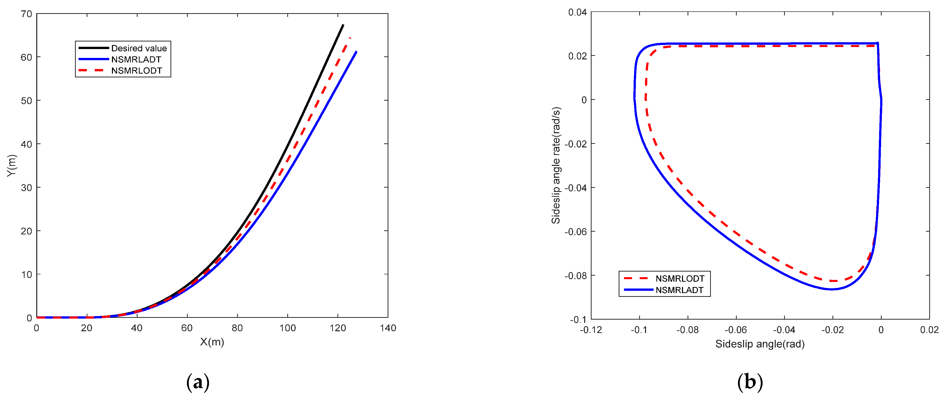
The simulation comparison results between NSMRLADT and NSMRLODT are shown in Figure 7. The vehicle track is given in Figure 7a. NSMRLADT and NSMRLODT can better track the desired trajectory path. Vehicles with ODT control have better lateral stability compared to ADT control. The phase diagram is shown in Figure 7b. The sideslip angle of the two methods is in the controllable range and presents a closed-loop convergence structure. Still, the overall control effect of NSMRLODT is superior to NSMRLADT. The ADT and ODT are shown in Figure 7c,d, respectively. The torque of the same side wheel under NSMRLADT control is the same, while the NSMRLODT control method can distribute the torque required to change among four respective in-wheel motors. It is possible to prevent the wheel with a small vertical load from quickly reaching the longitudinal force saturation. Although the torque distribution trend of the wheel on the same side under the NSMRLODT control method is the same, the amplitude is different. The front wheel torque is greater than the rear wheel torque, and this is because the front wheel is a steering wheel. As shown in Figure 7e, the sum of the load ratios of each wheel of NSMRLODT is smaller than that of NSMRLADT, indicating that the torque of each wheel is reasonably distributed under NSMRLODT. The maximum stability margin is kept as much as possible under the precondition of meeting the current yaw moment control. Leaving sufficient longitudinal force at the disposal of the car can make the vehicle more secure and reliable.
5.2. Performance Analysis under J-turn Maneuver
To further test the effectiveness of the proposed control strategy, we used the front steering angle for analog input, as shown in Figure 8.
The simulation results are shown in Figure 9, assuming driving at an initial speed of 80 km/h on a slippery road with an adhesion coefficient of 0.3.
The uncontrolled vehicle under the extreme road conditions of J-turn is unstable compared to the sinusoidal road conditions. In particular, the sideslip angle is worse than that of the SLC road condition. Compared with the uncontrolled vehicle’s yaw rate and sideslip curves, the CSMRLADT and NSMRLADT have converged the final tracking results. Still, the poor road conditions make the path tracking accuracy and stability poor. In contrast, the amplitude deviation of the yaw rate and sideslip angle is large, and there is chattering. The NSMRLODT effectively solves the chattering problem. The curves of yaw rate and sideslip angle are smoother and have suitable performance, which shows that the proposed control strategy can significantly improve yaw stability.
The simulation comparison results between NSMRLADT and NSMRLODT are shown in Figure 10. Note that the NSMRLODT introduced here is still effective in improving stability in extreme J-turn maneuvers. Based on the analysis of the above results, NSMRLODT is more suitable for the ideal state than NSMLRLADT.
6. Conclusions
The innovation of this paper is that new algorithms are proposed for the upper and lower controllers. In SMC, a more realistic 7DOF model is adopted, which contains two state variables, yaw rate and sideslip angle. NSMRL aims to reduce chattering and make sliding mode surface state variables converge faster. The lower controller adopts the utilization rate of four tires and its standard deviation coefficient as the objective function and prevents the stability margin gap between tires from being too large. The simulation results compare three hierarchical control strategies, CSMRLADT, NSMRLADT, and NSMRLODT, under single lane change and J-turn conditions. The comparison results show the NSMRLODT algorithm provides better trajectory tracking, and the torque of each wheel is reasonably distributed. The results show that the DYC control strategy designed in this paper can improve the system’s dynamic performance and tracking accuracy. At the same time, the stability and security of the system are considerably improved.
Author Contributions
Conceptualization, H.W. and J.H.; methodology, H.W. and J.H.; software, J.H. and H.Z.; validation, H.W.; formal analysis, H.W. and J.H.; investigation, H.W. and J.H.; resources, H.W. and J.H.; data curation, J.H.; writing—original draft preparation, J.H.; writing—review and editing, H.W.; visualization, H.W. and J.H.; supervision, H.Z.; project administration, H.W. All authors have read and agreed to the published version of the manuscript.
Funding
This work was supported by the Natural Science Foundation of China (grant no. 61903072), the Fundamental Research Funds for the Central Universities (grant no. N2223029), and the Higher Educational Science and Technology Program of Hebei Province (grant no. QN2019317).
Institutional Review Board Statement
Not applicable.
Informed Consent Statement
Not applicable.
Data Availability Statement
The data used in this study are self-text and self-collection.
Conflicts of Interest
The authors declare no conflict of interest.
References
- Subroto, R.K.; Wang, C.Z.; Lian, K.L. Four-wheel independent drive electric vehicle stability control using novel adaptive sliding mode control. IEEE Trans. Ind. Appl. 2020, 56, 5995–6006. [Google Scholar] [CrossRef]
- Chen, J.; Shuai, Z.; Zhang, H.; Zhao, W. Path following control of autonomous four-wheel-independent-drive electric vehicles via second-order sliding mode and nonlinear disturbance observer techniques. IEEE Trans. Ind. Electron. 2020, 68, 2460–2469. [Google Scholar] [CrossRef]
- Xie, X.; Jin, L.; Jiang, Y.; Guo, B. Integrated dynamics control system with ESC and RAS for a distributed electric vehicle. IEEE Access 2018, 6, 18694–18704. [Google Scholar] [CrossRef]
- Liang, Y.; Li, Y.N.; Khajepour, A.; Zheng, L. Holistic adaptive multi-model predictive control for the path following of 4WID autonomous vehicles. IEEE Trans. Veh. Technol. 2020, 70, 69–81. [Google Scholar] [CrossRef]
- Hang, P.; Xia, X.; Chen, X. Handling stability advancement with 4WS and DYC coordinated control: A gain-scheduled robust control approach. IEEE Trans. Veh. Technol. 2021, 70, 3164–3174. [Google Scholar] [CrossRef]
- Mok, Y.M.; Zhai, L.; Wang, C.; Zhang, X.; Hou, Y. A post impact stability control for four hub-motor independent-drive electric vehicles. IEEE Trans. Veh. Technol. 2022, 71, 1384–1396. [Google Scholar] [CrossRef]
- Lenzo, B.; Zanchetta, M.; Sorniotti, A.; Gruber, P.; De Nijs, W. Yaw rate and sideslip angle control through single input single output direct yaw moment control. IEEE Trans. Control. Syst. Technol. 2020, 29, 124–139. [Google Scholar] [CrossRef]
- Guo, H.; Liu, F.; Xu, F.; Chen, H.; Cao, D.; Ji, Y. Nonlinear model predictive lateral stability control of active chassis for intelligent vehicles and its FPGA implementation. IEEE Trans. Syst. Man Cybern. Syst. 2017, 49, 2–13. [Google Scholar] [CrossRef]
- Tahouni, A.; Mirzaei, M.; Najjari, B. Novel constrained nonlinear control of vehicle dynamics using integrated active torque vectoring and electronic stability control. IEEE Trans. Veh. Technol. 2019, 68, 9564–9572. [Google Scholar] [CrossRef]
- Ding, S.; Liu, L.; Zheng, W.X. Sliding mode direct yaw-moment control design for in-wheel electric vehicles. IEEE Trans. Ind. Electron. 2017, 64, 6752–6762. [Google Scholar] [CrossRef]
- Zhang, D.; Liu, G.; Zhou, H.; Zhao, W. Adaptive sliding mode fault-tolerant coordination control for four-wheel independently driven electric vehicles. IEEE Trans. Ind. Electron. 2018, 65, 9090–9100. [Google Scholar] [CrossRef]
- Zhao, X.; Chen, H.; Xie, S.G. Research on lateral control method of intelligent vehicle path tracking. Automot. Eng. 2011, 33, 382–387. [Google Scholar]
- Marino, R.; Scalzi, S.; Netto, M. Nested PID steering control for lane keeping in autonomous vehicles. Control. Eng. Pract. 2011, 19, 1459–1467. [Google Scholar] [CrossRef]
- Zhang, W.; Bai, W.; Wang, J.; Zhao, L.; Ma, C. Research on path tracking of intelligent vehicle based on optimal deviation control. Integr. Ferroelectr. 2018, 191, 80–91. [Google Scholar] [CrossRef]
- Hu, C.; Wang, R.; Yan, F.; Chen, N. Output constraint control on path following of four-wheel independently actuated autonomous ground vehicles. IEEE Trans. Veh. Technol. 2015, 65, 4033–4043. [Google Scholar] [CrossRef]
- Guo, J.; Luo, Y.; Li, K. An adaptive hierarchical trajectory following control approach of autonomous four-wheel independent drive electric vehicles. IEEE Trans. Intell. Transp. Syst. 2017, 19, 2482–2492. [Google Scholar] [CrossRef]
- Guo, J.; Luo, Y.; Li, K.; Dai, Y. Coordinated path-following and direct yaw-moment control of autonomous electric vehicles with sideslip angle estimation. Mech. Syst. Signal Processing 2018, 105, 183–199. [Google Scholar] [CrossRef]
- Peng, H.; Wang, W.; An, Q.; Xiang, C.; Li, L. Path tracking and direct yaw moment coordinated control based on robust MPC with the finite time horizon for autonomous independent-drive vehicles. IEEE Trans. Veh. Technol. 2020, 69, 6053–6066. [Google Scholar] [CrossRef]
- Krishna, S.; Narayanan, S.; Denis Ashok, S. Fuzzy logic based yaw stability control for active front steering of a vehicle. J. Mech. Sci. Technol. 2014, 28, 5169–5174. [Google Scholar] [CrossRef]
- Wu, L.; Su, X.; Shi, P. Sliding mode control with bounded 2 gain performance of Markovian jump singular time-delay systems. Automatica 2012, 48, 1929–1933. [Google Scholar] [CrossRef]
- Ding, S.; Li, S. Second-order sliding mode controller design subject to mismatched term. Automatica 2017, 77, 388–392. [Google Scholar] [CrossRef]
- Park, G.; Han, K.; Nam, K.; Kim, H.; Choi, S.B. Torque vectoring algorithm of electronic-four-wheel drive vehicles for enhancement of cornering performance. IEEE Trans. Veh. Technol. 2020, 69, 3668–3679. [Google Scholar] [CrossRef]
- Ohara, H.; Murakami, T. A stability control by active angle control of front-wheel in a vehicle system. IEEE Trans. Ind. Electron. 2008, 3, 1277–1285. [Google Scholar] [CrossRef]
- Shi, L.; Wang, H.; Huang, Y.; Jin, X.; Yang, S. A novel integral terminal sliding mode control of yaw stability for steer-by-wire vehicles. In Proceedings of the IEEE 37th Chinese Control Conference (CCC), Wuhan, China, 25–27 July 2018; pp. 7787–7792. [Google Scholar]
- Hamzah, N.; Aripin, M.K.; Sam, Y.M.; Selamat, H. Yaw stability improvement for four-wheel active steering vehicle using sliding mode control. In Proceedings of the IEEE 8th International Colloquium on Signal Processing and its Applications, Malacca, Malaysia, 23–25 March 2012; pp. 127–132. [Google Scholar]
- Ma, X.; Wong, P.K.; Zhao, J.; Xie, Z. Cornering stability control for vehicles with active front steering system using T-S fuzzy based sliding mode control strategy. Mech. Syst. Signal Processing 2019, 125, 347–364. [Google Scholar] [CrossRef]
- Zhang, H.; Liang, J.; Jiang, H.; Cai, Y.; Xu, X. Stability research of distributed drive electric vehicle by adaptive direct yaw moment control. IEEE Access 2019, 7, 106225–106237. [Google Scholar] [CrossRef]
- Alipour, H.; Bannae Sharifian, M.B.; Sabahi, M. A modified integral sliding mode control to lateral stabilisation of 4-wheel independent drive electric vehicles. Veh. Syst. Dyn. 2014, 52, 1584–1606. [Google Scholar] [CrossRef]
- Tota, A.; Lenzo, B.; Lu, Q.; Sorniotti, A.; Gruber, P.; Fallah, S.; Velardocchia, M.; Galvagno, E.; De Smet, J. On the experimental analysis of integral sliding modes for yaw rate and sideslip control of an electric vehicle with multiple motors. Int. J. Automot. Technol. 2018, 19, 811–823. [Google Scholar] [CrossRef]
- Acary, V.; Brogliato, B.; Orlov, Y.V. Chattering-free digital sliding-mode control with state observer and disturbance rejection. IEEE Trans. Autom. Control. 2011, 57, 1087–1101. [Google Scholar] [CrossRef]
- Mu, C.; Xu, W.; Sun, C. On switching manifold design for terminal sliding mode control. J. Frankl. Inst. 2016, 353, 1553–1572. [Google Scholar] [CrossRef]
- Mozayan, S.M.; Saad, M.; Vahedi, H.; Fortin-Blanchette, H.; Soltani, M. Sliding mode control of PMSG wind turbine based on enhanced exponential reaching law. IEEE Trans. Ind. Electron. 2016, 63, 6148–6159. [Google Scholar] [CrossRef]
- Li, J.; Yang, Y.; Hua, C.; Guan, X. Fixed-time backstepping control design for high-order strict-feedback non-linear systems via terminal sliding mode. IET Control. Theory Appl. 2017, 11, 1184–1193. [Google Scholar] [CrossRef]
- Deng, B.; Shao, K.; Zhao, H. Adaptive second order recursive terminal sliding mode control for a four-wheel independent steer-by-wire system. IEEE Access 2020, 8, 75936–75945. [Google Scholar] [CrossRef]
- Nojavanzadeh, D.; Badamchizadeh, M. Adaptive fractional-order non-singular fast terminal sliding mode control for robot manipulators. IET Control. Theory Appl. 2016, 10, 1565–1572. [Google Scholar] [CrossRef]
- Zhang, J.; Wang, H.; Zheng, J.; Cao, Z.; Man, Z.; Yu, M.; Chen, L. Adaptive sliding mode-based lateral stability control of steer-by-wire vehicles with experimental validations. IEEE Trans. Veh. Technol. 2020, 69, 9589–9600. [Google Scholar] [CrossRef]
- Tian, Y.; Cao, X.; Wang, X.; Zhao, Y. Four wheel independent drive electric vehicle lateral stability control strategy. IEEE/CAA J. Autom. Sin. 2020, 7, 1542–1554. [Google Scholar] [CrossRef]
- Asiabar, A.N.; Kazemi, R. A direct yaw moment controller for a four in-wheel motor drive electric vehicle using adaptive sliding mode control. Proc. Inst. Mech. Eng. Part K J. Multi-Body Dyn. 2019, 233, 549–567. [Google Scholar] [CrossRef]
- Jing, C.; Shu, H.; Song, Y.; Guo, C. Hierarchical control of yaw stability and energy efficiency for distributed drive electric vehicles. Int. J. Automot. Technol. 2021, 22, 1169–1188. [Google Scholar] [CrossRef]
- De Novellis, L.; Sorniotti, A.; Gruber, P. Wheel torque distribution criteria for electric vehicles with torque-vectoring differentials. IEEE Trans. Veh. Technol. 2013, 63, 1593–1602. [Google Scholar] [CrossRef] [Green Version]
- Abe, M. Vehicle Handling Dynamics: Theory and Application; Butterworth-Heinemann: Oxford, UK, 2015. [Google Scholar]
Figure 1.
Schematic diagram of 7DOF vehicle model.

Figure 2.
The force state of the wheel.
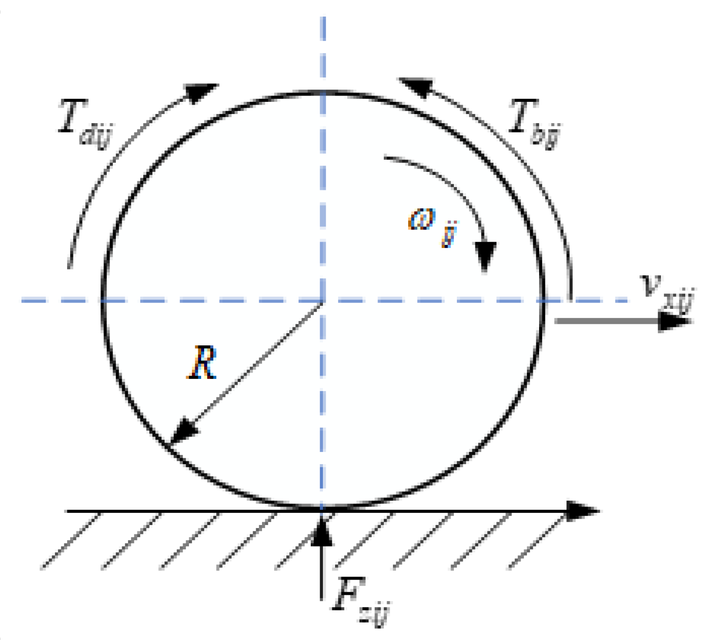
Figure 3.
Schematic diagram of 2DOF vehicle model.

Figure 4.
The schematic of the proposed control scheme.
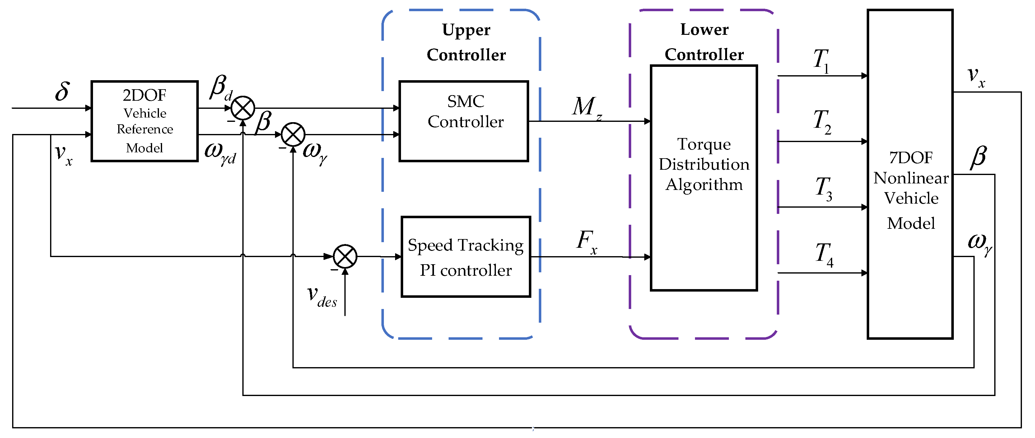
Figure 5.
Front wheel steering angle under SLC maneuver.
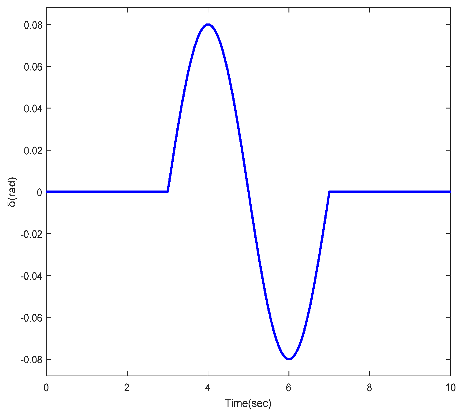
Figure 6.
The curves of yaw rate and sideslip angle under SLC maneuver. (a) Yaw rate; (b) sideslip angle.
Figure 6.
The curves of yaw rate and sideslip angle under SLC maneuver. (a) Yaw rate; (b) sideslip angle.
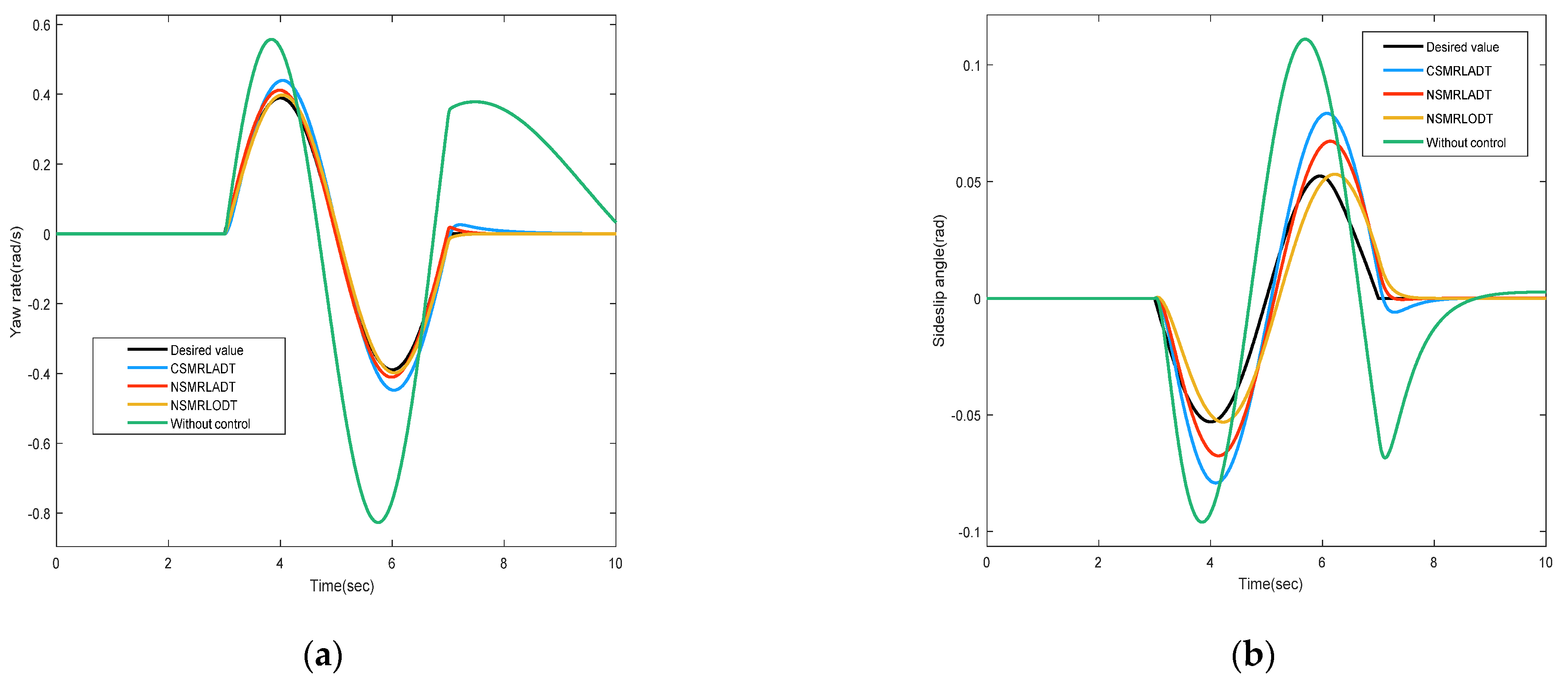
Figure 7.
Simulation comparison of NSMRLADT and NSMRLODT under SLC maneuver. (a) Vehicle trajectory; (b) phase planes; (c) ATD; (d) ODT; (e) total load rate of the four tires.
Figure 7.
Simulation comparison of NSMRLADT and NSMRLODT under SLC maneuver. (a) Vehicle trajectory; (b) phase planes; (c) ATD; (d) ODT; (e) total load rate of the four tires.
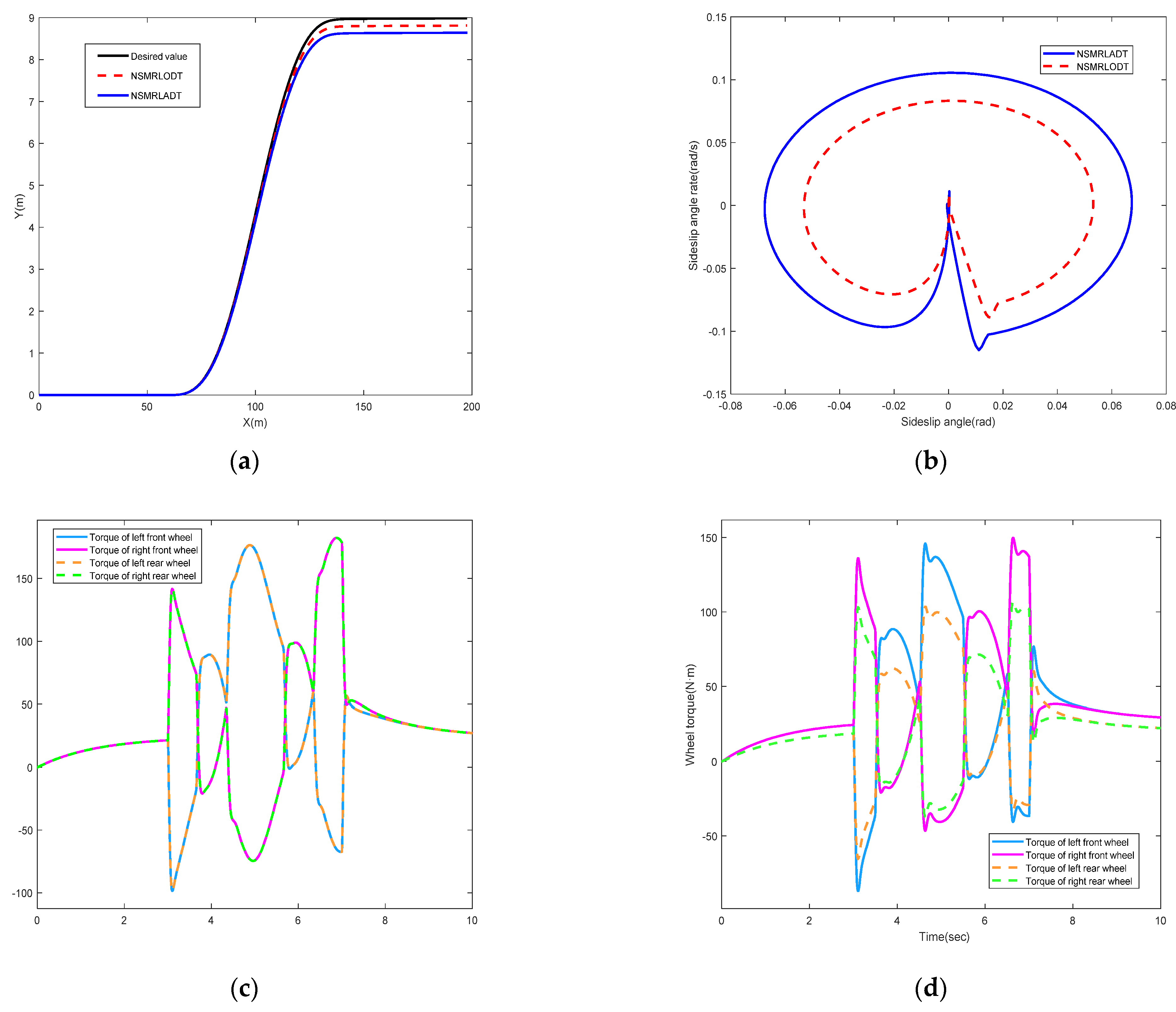
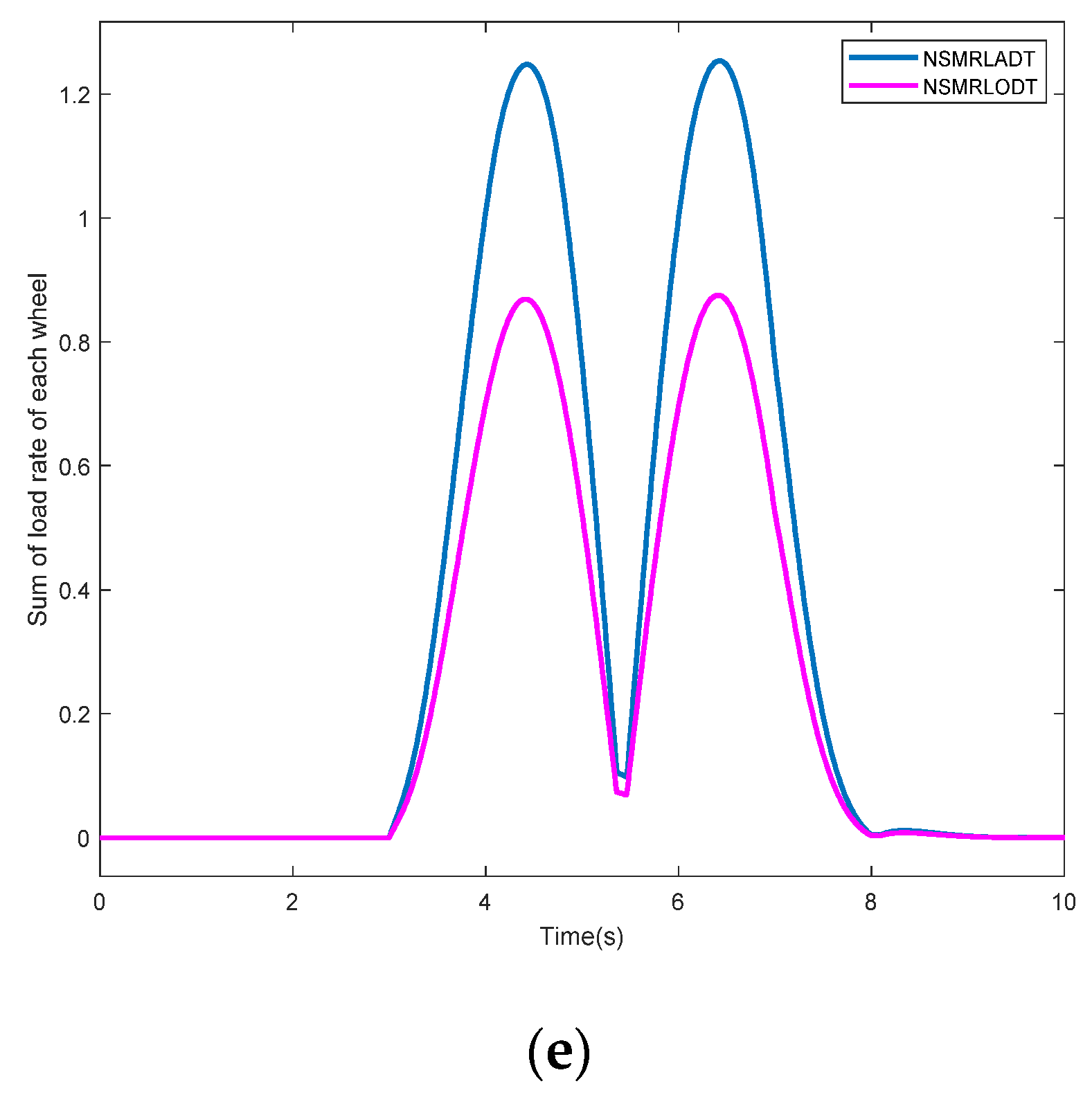
Figure 8.
Front wheel steering angle under J-turn maneuver.

Figure 9.
The curves of yaw rate and sideslip angle under J-turn maneuver. (a) Yaw rate; (b) sideslip angle.
Figure 9.
The curves of yaw rate and sideslip angle under J-turn maneuver. (a) Yaw rate; (b) sideslip angle.
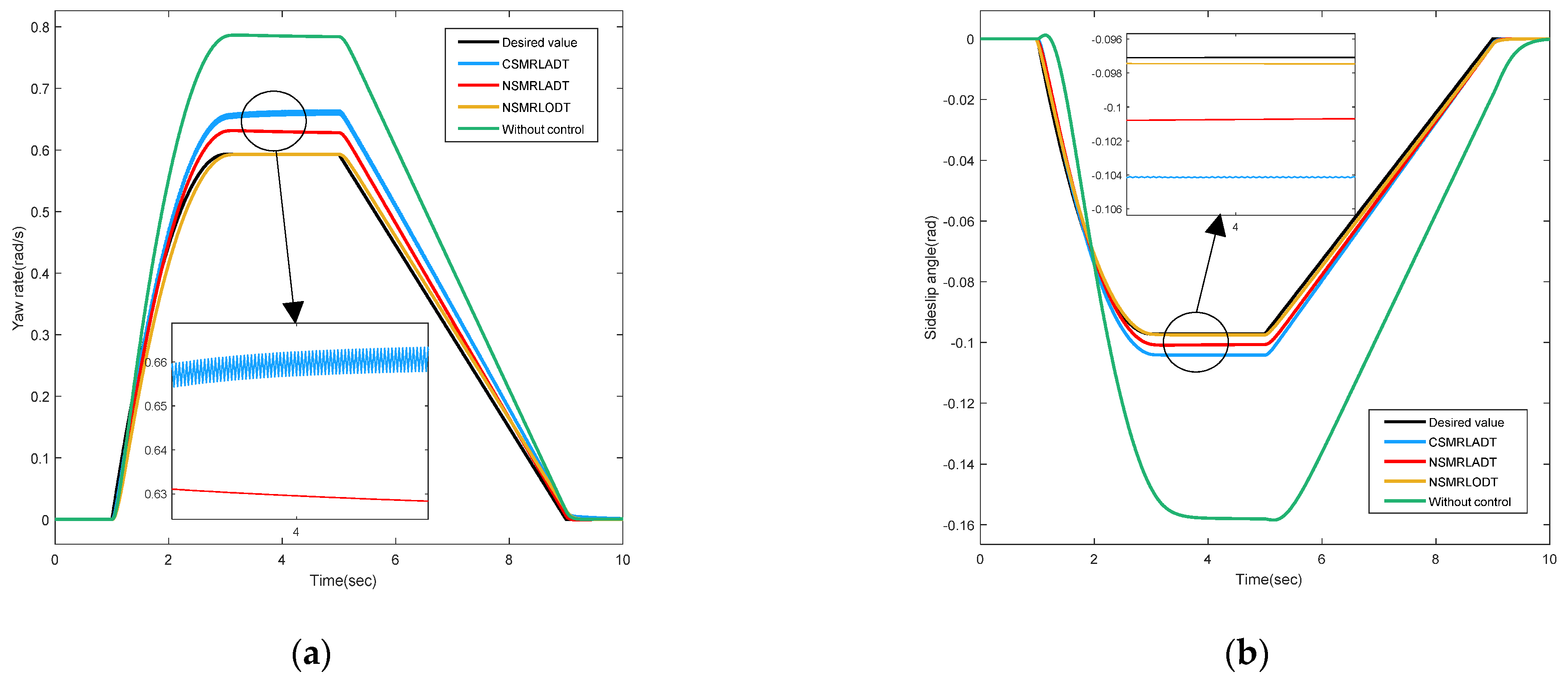
Figure 10.
Simulation comparison of NSMRLADT and NSMRLODT under J-turn maneuver. (a) Vehicle trajectory; (b) phase planes; (c)ADT; (d) ODT; (e) total load rate of the four tires.
Figure 10.
Simulation comparison of NSMRLADT and NSMRLODT under J-turn maneuver. (a) Vehicle trajectory; (b) phase planes; (c)ADT; (d) ODT; (e) total load rate of the four tires.


Table 1.
Lagrange multiplier method.
| Lagrange Multiplier Method |
|---|
| By introducing slack variables , inequality constraints are transformed into equality constraints |
| where are the Lagrange computing factors, is introduced to ensure that it is non-negative, so that the constraint function is less than or equal to zero is satisfied. |
| The derivative of with respect to each variable is 0 , By solving the equations above, we can obtain . |
Table 2.
Vehicle parameters.
| Description | Symbol | Value |
|---|---|---|
| Total mass of the car vehicle | 1480 (kg) | |
| Distance from front axle to the center of centroid | 1.2 (m) | |
| Distance from rear axle to the center of centroid | 1.4 (m) | |
| Yaw moment of inertia of vehicle | 1523 (kg) | |
| Moment of inertia of the wheel | 2.1 (kg) | |
| Distance from the center of centroid to ground | 0.5 (m) | |
| Front track width | 1.6 (m) | |
| Rear track width | 1.6 (m) | |
| Rolling radius of the tire | 0.354 (m) | |
| Front wheel cornering stiffness | 35796 (N/rad) | |
| Rear wheel cornering stiffness | 35400 (N/rad) | |
| Peak torque of the motor tire | 400 (N) | |
| Rolling resistance coefficient | 0.018 |
Publisher’s Note: MDPI stays neutral with regard to jurisdictional claims in published maps and institutional affiliations. |
© 2022 by the authors. Licensee MDPI, Basel, Switzerland. This article is an open access article distributed under the terms and conditions of the Creative Commons Attribution (CC BY) license (https://creativecommons.org/licenses/by/4.0/).
Share and Cite
MDPI and ACS Style
Wang, H.; Han, J.; Zhang, H. Lateral Stability Analysis of 4WID Electric Vehicle Based on Sliding Mode Control and Optimal Distribution Torque Strategy. Actuators 2022, 11, 244. https://doi.org/10.3390/act11090244
AMA Style
Wang H, Han J, Zhang H. Lateral Stability Analysis of 4WID Electric Vehicle Based on Sliding Mode Control and Optimal Distribution Torque Strategy. Actuators. 2022; 11(9):244. https://doi.org/10.3390/act11090244
Chicago/Turabian StyleWang, Hongwei, Jie Han, and Haotian Zhang. 2022. "Lateral Stability Analysis of 4WID Electric Vehicle Based on Sliding Mode Control and Optimal Distribution Torque Strategy" Actuators 11, no. 9: 244. https://doi.org/10.3390/act11090244
Note that from the first issue of 2016, this journal uses article numbers instead of page numbers. See further details here.