Building Energy Assessment and Computer Simulation Applied to Social Housing in Spain
by
 , , , and
Juan Aranda
1 ,
,
Ignacio Zabalza
2,* ,
,
Eva Llera-Sastresa
2,
Sabina Scarpellini
3 and
Alfonso Alcalde
1 1
CIRCE Foundation, Campus Río Ebro, Calle Mariano Esquillor Gómez, 15, 50018 Zaragoza, Spain
2
Department of Mechanical Engineering and CIRCE Research Institute, University of Zaragoza, Calle María de Luna, 5, 50018 Zaragoza, Spain
3
Department of Accounting and Finance and CIRCE Research Institute, University of Zaragoza, 50009 Zaragoza, Spain
*
Author to whom correspondence should be addressed.
Buildings 2018, 8(1), 11; https://doi.org/10.3390/buildings8010011
Submission received: 31 October 2017
/
Revised: 15 December 2017
/
Accepted: 11 January 2018
/
Published: 16 January 2018
Abstract
:The actual energy consumption and simulated energy performance of a building usually differ. This gap widens in social housing, owing to the characteristics of these buildings and the consumption patterns of economically vulnerable households affected by energy poverty. The aim of this work is to characterise the energy poverty of the households that are representative of those residing in social housing, specifically in blocks of apartments in Southern Europe. The main variables that affect energy consumption and costs are analysed, and the models developed for software energy-performance simulations (which are applied to predict energy consumption in social housing) are validated against actual energy-consumption values. The results demonstrate that this type of household usually lives in surroundings at a temperature below the average thermal comfort level. We have taken into account that a standard thermal comfort level may lead to significant differences between computer-aided energy building simulation and actual consumption data (which are 40–140% lower than simulated consumption). This fact is of integral importance, as we use computer simulation to predict building energy performance in social housing.
1. Introduction
For most EU member states, there is a general consensus nowadays that energy poverty in households is a top priority which should be addressed to avoid social exclusion. This issue has been tackled by ensuring that most citizens can access energy at stable and affordable prices [1]. Indeed, the European Commission in the recent “Winter Package” (2016) [2] has acknowledged this issue. The issue of energy poverty is more severe in Southern and Eastern Europe [3]. Despite more favourable climatic conditions in Southern Europe, 16.6% of households in the Mediterranean region live in conditions characterised by poor thermal comfort; in contrast, the European average is 4% lower [4].
Owing to its importance for policy-formulation purposes, energy poverty has been defined by many authors [5]. The International Energy Agency [6] states that a household is in a situation of “energy poverty” when it has to pay energy costs which are excessive compared to the total household income. The definition provided by the International Energy Agency (IEA) is very similar to that adopted by the Environmental Sciences Association (ACA) in a pioneering Spanish publications [7]. Energy poverty is a particular type of poverty which is principally determined by various factors [8]: the ratio of minimum annual energy expenditure to income in a household [9], the energy efficiency of buildings [10], and finally the (more subjective) perception of comfort level in the dwelling [11]. Authors such as Rudge [12] establish this adequate level of comfort in a dwelling as an indoor temperatures ranging between 18 °C and 21 °C in winter, and a constant humidity level ranging between 20% and 80% of relative air humidity. Comfort level is affected by the clothing of the residents, the air speed and the level of physical activity and can only be expressed statistically by means of psychometric diagrams, due to the subjective nature of this parameter [13].
These definitions include a subjective component, such as the thermal comfort level or satisfactory living conditions. To solve this issue, Grevisse and Brynart [14] define “energy poverty” as the inability of a household to meet its certified energy needs. In this case, the subjective component means that an assessment and certification by a competent Public Body is necessary, as this body can confirm and classify the degree of vulnerability of the different households in terms of energy [8]. In Spain, this evaluation and certification is provided locally by regional Public Social Services.
Based on the fundamental contribution by Boardman [15], we applied the following information in our study: the use of 10% of net income to sufficiently meet energy needs is used as an index to detect households living with energy poverty. This figure was also applied by Taylor [16], who introduced into the debate the definition of “energy poverty” [17]. This threshold of 10% of annual net income being used to cover basic energy expenditure is a clear and measurable limit, and has been used in this present study to identify energy poverty in social housing.
Certain structural aspects of the global energy system help to sustain energy poverty, according to Sovacool [18]. In general terms, a higher number of cases of energy poverty may occur among groups living in social housing, mainly due to the lower average level of income of these households. The influence of energy poverty on social housing has been studied by several authors in different countries, cities and climate zones such as in Australia [19], the United Kingdom [20,21], the Netherlands [22], and in several areas of Spain [10,23,24].
Social housing is also a useful area of study in terms of examining the usage habits of the residents, specifically the comfort temperature target or the heating schedules. These users’ patterns make them different from the average urban households of European cities, according to Teres-Zubiaga et al. [10] and Hui Ben and Steemers [25]. The report “Energy poverty and vulnerable consumers in the energy sector across the EU: analysis of policies and measures” by the European Commission [26] indicated that social housing has been the main focus of several initiatives, perhaps because of the high level of energy poverty of its occupants (this is in line with the conclusions reached by Hills [9] and Li et al. [27]).
Energy-simulation tools have been mainly applied when refurbishment of social housing is being analysed, as energy refurbishment has a greater social impact in those cases where residents are living with energy poverty [11]. Despite the many improvements in computer-simulation techniques, the specificities of social housing still cause variations between the results obtained by computer simulation and the actual energy consumption in these dwellings, as Tronchin and Fabbri [28], Wang and Zhai [29] and Escandón et al. [30] have pointed out. These differences may not be of great import in, for example, the energy certification of buildings, where the object of the study is a building which is generally compared to a reference building with similar characteristics, geometry, occupancy, use, and which is built in areas with the same climatic conditions. However, these differences are very important when simulation is carried out to assess the energy savings and benefits associated with building refurbishment and related investments [31], or to define the priorities of public bodies providing subsidies for social housing based on the buildings’ energy performance [32]. Ramos et al. [33] state that the differences in energy performance are mainly related to specific social housing constraints. Efficient technologies alone cannot fix the problem, unless these technologies are adequately combined with an understanding of sociological aspects [34].
Energy simulation is a widely extended tool which is used to assess energy performance in a building; it could also be used to evaluate energy poverty. However, using the simulation results with predetermined user profiles to assess the root causes of energy poverty, or to note energy-efficient refurbishment measures, may lead to important errors [31].
This study analyses the application of energy-simulation tools to a sample of social housing in Spain. The main contribution of this article lies in the comparative analysis of real patterns of energy consumption in social housing. This analysis was undertaken to identify the variables that influence the level of energy poverty of these households and the causes of deviations in the data (computer simulations vs actual data). The obtained results can be used to improve the accuracy of the energy-performance simulations of a building of social houses: a characterisation of users’ patterns in buildings, where most of the households are somehow affected by energy poverty, can thus be undertaken [35].
The article comprises two analyses. The first is an empirical analysis of energy-consumption patterns and energy-poverty assessment in a sample of social housing in Spain. The second analysis focuses on the use of energy-simulation tools to assess energy poverty (applied to the same sample). We will also take into account the limitations of these tools when studying social housing in Spain, and make recommendations based on our in-depth study of the issue of energy poverty.
2. Methodology
Cases of energy poverty are associated with households in the present study. For our purposes, the household is the analytical unit with which we aim to tackle energy poverty. This approach is in line with that of Webb et al. [36].
Buildings play a major role in energy demand. For each specific climate, the energy demand of a building is related to the construction of the building and depends on factors such as materials, insulation, as well as the building’s geometry and the level of exposure to wind and sun radiation. Fully dedicated social housing building units are considered in the analysis. To discriminate energy poverty cases, a threshold of 10% of total annual income being used to satisfy energy needs, as postulated by Boardman [15], was applied here. This index is easy to calculate using the available data and allows us to consider the relationship between excessive energy costs and household net income.
The first step for this study involved setting the selection criteria used to search for social housing samples. Buildings had to be homogenous in terms of their age, construction, maintenance and management, function and the climate of their setting. Two blocks of fully dedicated social housing apartments were selected (noted as buildings A and B). They are located in the city of Zaragoza (Spain) and are of public ownership; they are managed by the municipal company “Zaragoza Vivienda”, which reports to the Zaragoza City Council. Both buildings are subject to the same climatic conditions, were built at the same time in 1988, and are close to the average municipal housing stock age (from 1985). They have the same maintenance policy since they are publicly owned, and are used for the same purpose (public social housing for rent).
Two types of complementary and comparative analyses were performed in the present study: an empirical analysis which was used to analyse energy poverty in the sample based on actual energy consumption data, and an energy-performance simulation which was used to validate this approach as a tool with which to assess energy poverty.
2.1. Empirical Analysis
An empirical analysis of the data for each building was undertaken to characterise the energy consumption associated with this type of social housing. Four main types of variables have been studied: building envelope and geometric characteristics, energy-consuming equipment, energy sources and energy consumption, and household structure and consumption patterns (Table 1).
The public company managing the buildings provided data on building materials and construction details, refurbishments carried out to date and the precise dimensions of the various floors and rooms (Subsections 1 and 2 in Table 1).
A survey addressed to the building residents, which included socio-economic questions, was designed and distributed to all households. The questionnaire included questions about the household structure, residents’ employment and social situations, energy usage habits, the residents’ schedules and the intensity of use of the energy-consuming elements (Subsections 3 and 4 in Table 1).
In total, 36 households out of 160 participated in the survey in building A, and 8 out of 12 participated in building B. The obtained sample was validated against the following criteria:
- The different occupancy levels of the dwellings had to be taken into account, to permit us to study the effects of family structure and occupancy. The sample includes between two and six dwellings for each occupancy level (from one to seven people).
- The different orientations of the buildings and the types of dwelling in each building were accounted for. Building B has three floors with four different types of dwellings per floor: two north facing and two south facing. The sample includes two dwellings of each type, distributed over three floors.
In addition, a detailed energy audit of two dwellings was carried out for each building analysed to confirm and extend the available data for the dwellings. This audit included a visit to the dwellings to measure and collect data on the indoor temperature, relative humidity, thermal transmittance of the building envelope and details relating to the residents’ energy-consumption habits such as their schedules, their usage of HVAC equipment, as well as the number and type of household appliances.
2.2. Energy Simulation
Energy simulations using computer tools and reputable commercial databases were carried out on these social housing buildings. The EnergyPlus calculation engine was used along with the DesignBuilder V4.7 (Stroud, Gloucestershire, UK) interface [37]. The characteristics of the building and its enclosures, the equipment of the building and an average-user profile were modelled based on survey data and data supplied by the management company. Three different user profiles were created, according to the most common schedules registered: Families with 4 members, adults working full-time; families with 4 members, adults unemployed; and families with 2 members, adult(s) working part-time.
Finally, the simulation model was validated by comparing simulation results with actual energy consumption. Significant differences were noted, and, on this basis, we revised the model input parameters to fine-tune the model. A sensitivity analysis that included several model parameters was completed to assess the margin of error when using inaccurate input data. The user profiles and thermal comfort levels [38,39] received most attention, and we took into account the type of housing analysed.
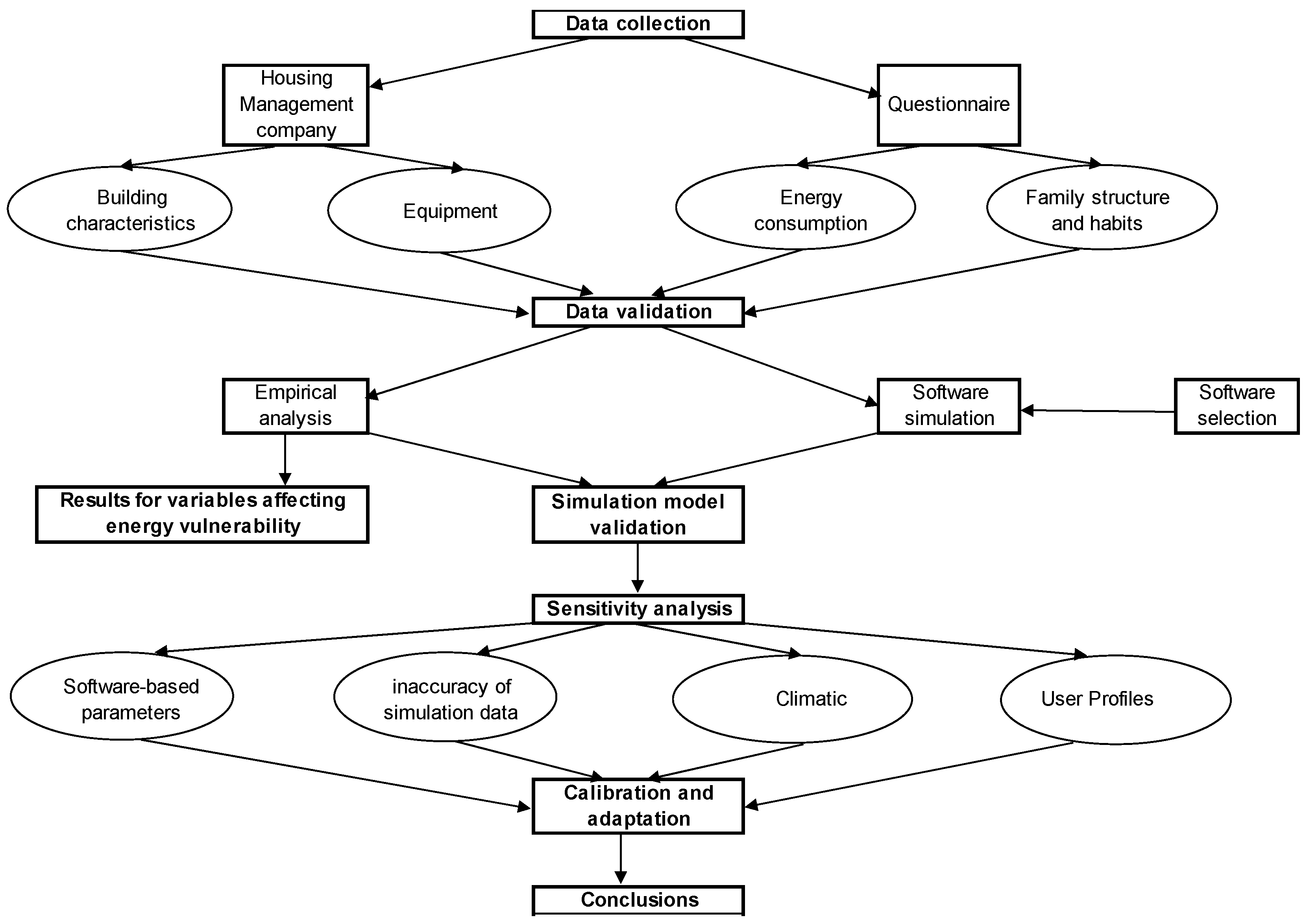
Figure 1 summarises schematically the methodology followed in this study.
3. Case Study
Social housing in Spain has particular characteristics, both in terms of the buildings themselves and in their maintenance. A large percentage of these residential buildings were built prior to the implementation of the first energy-efficiency regulations in buildings [30]. As few major retrofitting works have been carried out, these buildings usually have little or no insulation. Owing to the mild winter climate of the region and the poor gas-grid development at the time of construction, heating systems are individual and usually run on electricity. Public social housing, which constitutes a small proportion of the total social housing stock [40] is well maintained and managed by the public authorities (usually municipal); there is no evidence that private social housing undergoes regular maintenance or building upgrades owing to the low rent of this type of housing.
Two buildings have been chosen for this study because they are homogeneous and representative of social housing in the city of Zaragoza (Aragon region of Spain); they also present interesting differences, mainly in relation to their size and HVAC equipment. The two buildings consist of individual apartments for residential use, with levels of occupancy generally ranging between one and seven people on low income. The dwellings are between 40 and 70 m2. The buildings were built in 1988; at that time, few energy-efficiency criteria were contained in the regulations [41]. All the dwellings are in the same climatic zone (mild Mediterranean). Building A is a group of blocks with 160 dwellings over eight floors, while building B consists of a single block of twelve dwellings over three floors. Another relevant difference is the individual heating system that runs on gas boilers in building A, and electric resistance radiators in building B.
Many family units have been subject to detailed attention by public social services, and, in some cases, they have received additional emergency aid to cover the minimum expenses of housing (mainly rent), and energy expenses, as well as other basic needs.
The climate in Zaragoza is dry and continental Mediterranean with very low rainfall, mild winters and hot summers. The average temperature is 15.5 °C. The registered number of annual Heating Degree Days (HDD), using a reference temperature of 15 °C [42], is 1177 HDD (Degree days calculated using www.degreedays.net). The average wind speed is 19 km/h. The predominant wind is cold and dry, blowing in a Northwest–Southeast direction [43].
Table 2 describes the building characteristics, which are relevant from an energy-performance point of view.
From the point of view of construction quality, both buildings have no thermal insulation, but both comply with the Basic Norms of Buildings in force in the year of construction [41]. Transmittances values of the main enclosing areas are shown in Table 3, along with the limits of the current building regulations CTE DB HE1 [44] corresponding to the climatic zone D3 (“D” indicates the winter-weather severity on a scale from A to E and “3” indicates the summer weather severity on a scale of 1 to 4). Looking at the value of the transmittances, building B exhibits better enclosure quality. A recent refurbishment of building B improved insulation, and adapted it to the aforementioned regulation.
As for the structure of the households in each building, there was a higher level of average occupancy in building A than in building B. There was more average living space per person in building B (28.5 m2/person) than in building A (18.5 m2/person) despite the smaller size of the average dwelling.
A similar average level of income was noted for households in both buildings, as shown in Table 4. The level of income was slightly above the “poverty threshold” established in Spain at €7961/year for a one-person household, according to the 2015 Living Conditions Survey by the National Institute of Statistics [45]. The income level is also below the “poverty line” for four-person households in Spain (€16,719/year), and well below the average income of households in Zaragoza, which is €24,336/year [46]. However, a few relatively high values strongly distort this distribution, as 38% of the households in building A and 25% in building B are living below the poverty line [45].
Energy poverty is a type of economic poverty that affects the basic consumption of households. The main cause of energy poverty is a lack of economic resources, as has been noted in Scarpellini et al. [8]. The number of employed household members significantly affects the energy consumption of households: it is higher in building A (0.7 employed per household vs 0.4 in building B), but it should be noted that those employed in building A earned lower average wages.
Regarding the equipment, neither of the two buildings has summer cooling systems, and residents use natural and mechanical ventilation to improve their thermal comfort at home. This lack of cooling equipment is common to all social housing in Southern Europe [47]. The demand for heating takes place over longer periods, carries more health risks and produces a greater sense of dissatisfaction in its absence than an absence of cooling. In addition, there are alternative solutions to a lack of cooling equipment, such as ventilation during cooler hours, limiting thermal gains with curtains and blinds, and the potential to act on parameters such as “activity”, “clothing”, and “humidity” with evaporative coolers, and the “speed of air” using fans. Therefore, although there is a demand for cooling in both buildings, no consumption derived from cooling was considered.
For heating and Domestic Hot Water (DHW), building A has 24-kW individual gas condensing boilers, with a rated throughput of between 87.8% and 92.8%, depending on the type, and a variable operating schedule which is set individually by each user. These boilers are gradually replacing the original gas boilers with a nominal throughput of 72%. Each dwelling has a central thermostat that regulates the heating, and manual valves to open and close the radiators of each room. During the energy audit, it was possible to verify that the lack of maintenance produced lime deposits in the valves that impeded the correct operation of the valves. The gas supply is individual and may also be used in the kitchen, although most of the residents have electric glass-ceramic cookers. The rest of the energy consumption is related to electrical equipment.
Building B has individually-manoeuvrable resistance electric-heating systems. The DHW is provided by individual electric-resistance tanks of between 30 and 70 L capacity. In addition, households own a variety of portable electric-heating apparatus. This led to a larger electrical power-supply capacity in building B, where the average is in 5.6 kW of contracted power compared to the average 3.5 kW in building A. This increased the fixed energy costs of residents in building B for the same energy consumption.
4. Results and Discussion
4.1. Energy Poverty: An Empirical Analysis
Average actual energy consumption per month has been evaluated for 2015. As can be observed in Figure 2 and Table 5, a higher energy consumption per dwelling was detected in building A. Energy consumption in building A was 47% greater than in building B because of the larger dwelling size (25%) and the partial envelope refurbishment that had been undertaken in building B. However, the energy cost for those dwelling in building B was 18% higher than for those residents of building A. Whereas only electricity was consumed in building B, building A’s thermal demand (66%) was met by natural gas. The average energy price (fixed cost and tax included) of the gas-electricity combination in building A is €0.11/kWh, while in building B the electricity price is €0.2/kWh. These costs (especially the electricity costs) are among the highest in the European Union according to Bouzarovski [48], owing to the excessively regulated electricity sector in Spain. Therefore, there is a strong link between the source of the energy used in a dwelling and its cost, especially since electricity is indispensable but economically inefficient for thermal purposes when compared to other energy sources, such as natural gas or biomass [49].
In terms of energy consumption per useable area, building B presents a lower ratio than building A: 77.5 kWh/m2 year compared to 87.6 kWh/m2 year. This ratio reflects the better energy performance of building B. It is more efficient because it is a more compact building, with a lower height and a smaller glazed area. In this building, half of the windows are composed of double-glazing and PVC-framed windows, which are much more efficient than the single-glazed aluminium frame windows of building A. However, the difference in energy consumption of these buildings is not as great as might be expected: we should take into account that the thermal-transmittance values are higher than the design values in building B. External wall insulation level is a key factor in a building’s energy demand performance [50]. In building B, the measured thermal transmittance of the outer walls (0.91 W/m2K) was much higher than the refurbishment target value (0.27 W/m2K) and even higher than the measured value in building A (0.71 W/m2K).
If we compare these energy-consumption figures with those of an average dwelling in a Mediterranean climatic zone in Spain (121.45 kWh/m2 year, according to the Institute for Diversification and Energy Saving (IDAE) [51]), these social houses use between 39% and 57% less energy, although there is no evidence for better energy performance (see Table 6).
The average dwelling in building A consumes less energy than an average four-person household in Spain, with 4.4 kW of electrical contracted power and an annual energy consumption of 3900 kWh (only electricity) [8]; this is similar to the level of consumption of building B. Indeed, the unit cost for the electricity consumed (€/kWh) is similar in all cases, since the contracted power savings (fixed costs) are masked by the higher electricity consumption.
A survey conducted by Scarpellini et al. in 2014 [8] on a sample of social housing in Aragon revealed that, in general, people at risk of energy poverty, are largely unaware of energy-supply contract types or details. In fact, the majority (70%) of people in this type of housing had the standard regulated tariff for domestic consumers (PVPC: Precio de Venta a Pequeño Consumidor. Regulated electricity tariff for domestic sector in Spain), and paid a fixed charge for a high contracted power, that they did not need. Only 15% of the households in building B requested a reduction in their contracted power to adapt the supply to their needs and thus reduce electricity costs. This result is in line with the low level of social tariff applications by social housing residents: thus, not many residents benefit from discounts for vulnerable households, according to another survey of social housing residents in the same region of Aragon, by Scarpellini et al. (2017) [52].
Energy poverty may often be caused by a combination of the energy performance of the building (thermal envelope-demand and equipment-consumption), the energy source used and the dwelling size. In the case studies presented, the dwellings of building B are more efficient (13% lower relative consumption) and are smaller (25% smaller on average), but the energy costs per dwelling are 18% higher. Although the energy-consumption habits can be improved through training and user feedback programmes [53,54], improving the heat-generation systems and redesigning energy tariffs should be a priority in these households, before proposing expensive solutions to refurbish the thermal envelope. The increase in electricity prices in many European countries has aggravated the vulnerability of many low-income and energy-inefficient households [55]. In these cases, the use of natural gas for heating systems presents some beneficial results [56]. Providing a more diversified range of primary energy sources can also contribute to alleviate energy-poverty status [57].
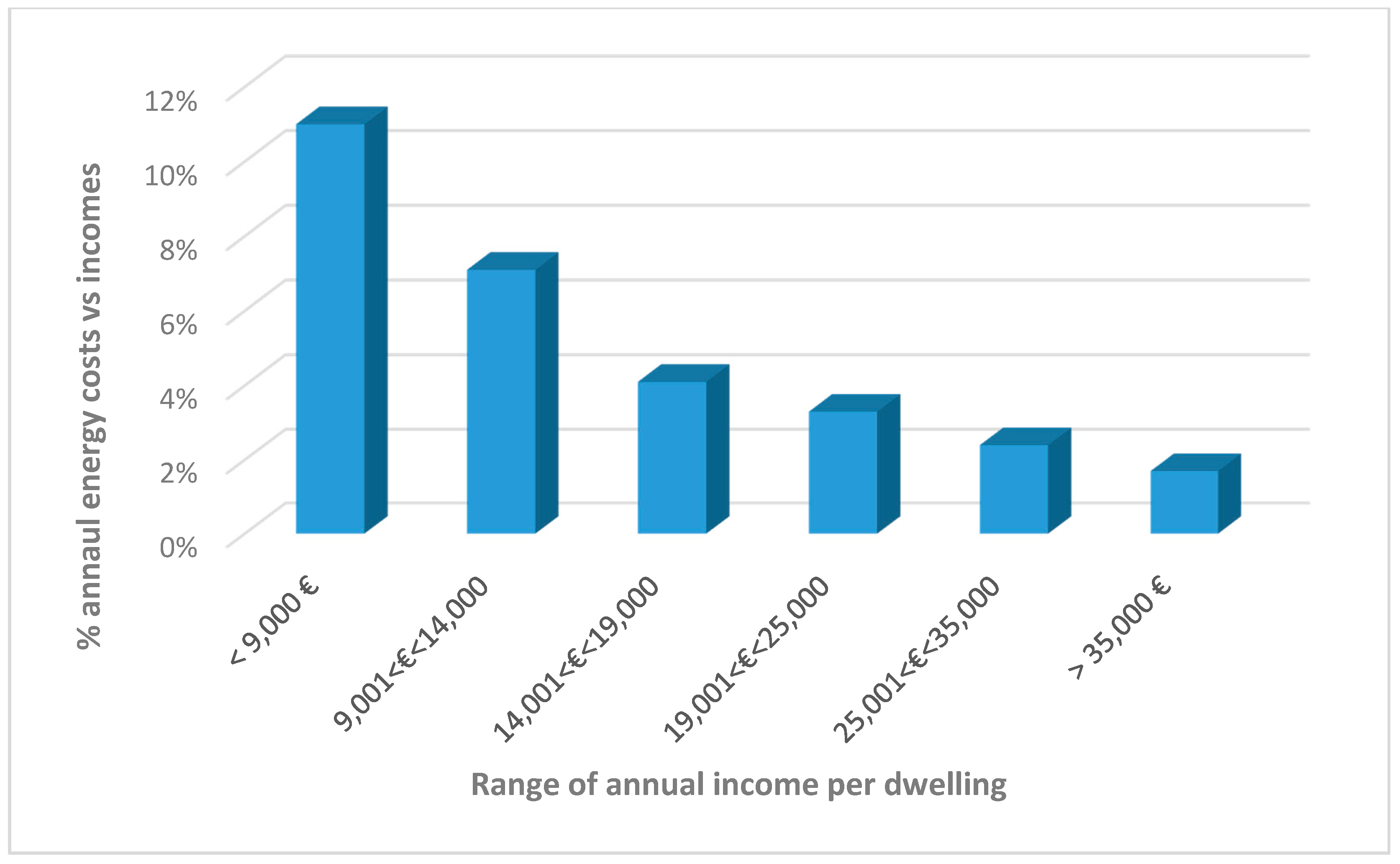
Residents in building A spent on average 6.1% of their income on energy costs, whereas an average household spent between 2% and 4%. Owing to the higher energy costs of building B, this indicator rises to 6.7%. Figure 3 indicates the ratio of annual energy costs versus the annual income, disaggregated by income levels. Most of the households whose income vs energy cost ratio exceeded 10% have annual incomes lower than €9000/year, which demonstrates that income is the greatest factor for energy poverty.
Any energy renovations should ensure improvement occurs in three fundamental areas. In order of importance, these are: energy poverty, energy consumption of buildings, and mitigation of climate change [58]. As reported by Teli et al. [59], the savings derived from energy refurbishment in social housing are much lower than those in standard housing. The most significant result of energy refurbishment is the social benefit achieved by the improvement of the thermal comfort conditions in the refurbished dwelling, as this increases health and life quality of the residents, as noted by Ormandy and Ezratty [60]. Investments may consider building-envelope retrofitting and heating-equipment replacement, but only the former translate into energy-poverty alleviation and indoor-comfort improvements [61]. These investments should be undertaken by the public entity that owns the dwellings [31], and the improvements should be included in a holistic programme of refurbishing and improving social housing, as noted by Swan et al. [62].
4.2. Energy Simulation Results
Computer-aided energy simulation has proven to be a fast, economic and accurate method of predicting energy consumption in a building and assessing the benefits of building refurbishment [63,64]. The energy simulation of the building begins with modelling the geometry and composition of the thermal envelope of the buildings, as well as the building’s internal zoning (using the engine tool EnergyPlus). The internal zones are divided into habitable zones separated by adiabatic walls and non-habitable common zones separated by internal partitions. The vertical enclosure in building A is composed of exterior walls, whereas building B also has two walls that are shared with the neighbouring buildings, as can be noted in Figure 4.
After the modelling of the building installations and equipment, an average user profile was modelled, defining a temperature set-point for heating (20 °C) during the winter and a temperature set-point for cooling (26 °C) during the summer. The summer target temperature did not involve any additional energy consumption because there are no cooling systems in either of the buildings. No precise data is available for setting the ventilation rate. In both buildings, a value of 1.5 ac/h (including leaks) was considered. This value is quite common in this type of building, although it is more than twice the reference value for energy certification of existing buildings in Spain (0.63 ac/h according to Royal Decree 235/2013 [65]). Moreover the value considered was higher than the average ventilation rates for renovated buildings, ranging from 0.35 to 1.01 ac/h in the study published by Ramos et al. [66].
The heating-user profile was developed based on questionnaires and interviews conducted with residents. In both buildings, the heating schedule is set manually by residents, and we presumed that there is no consumption of energy when residents are away from home. Based on the information provided in the interviews, there is no night-time heating consumption, and all heating systems are turned off from 11:00 p.m. to 7:00 a.m.
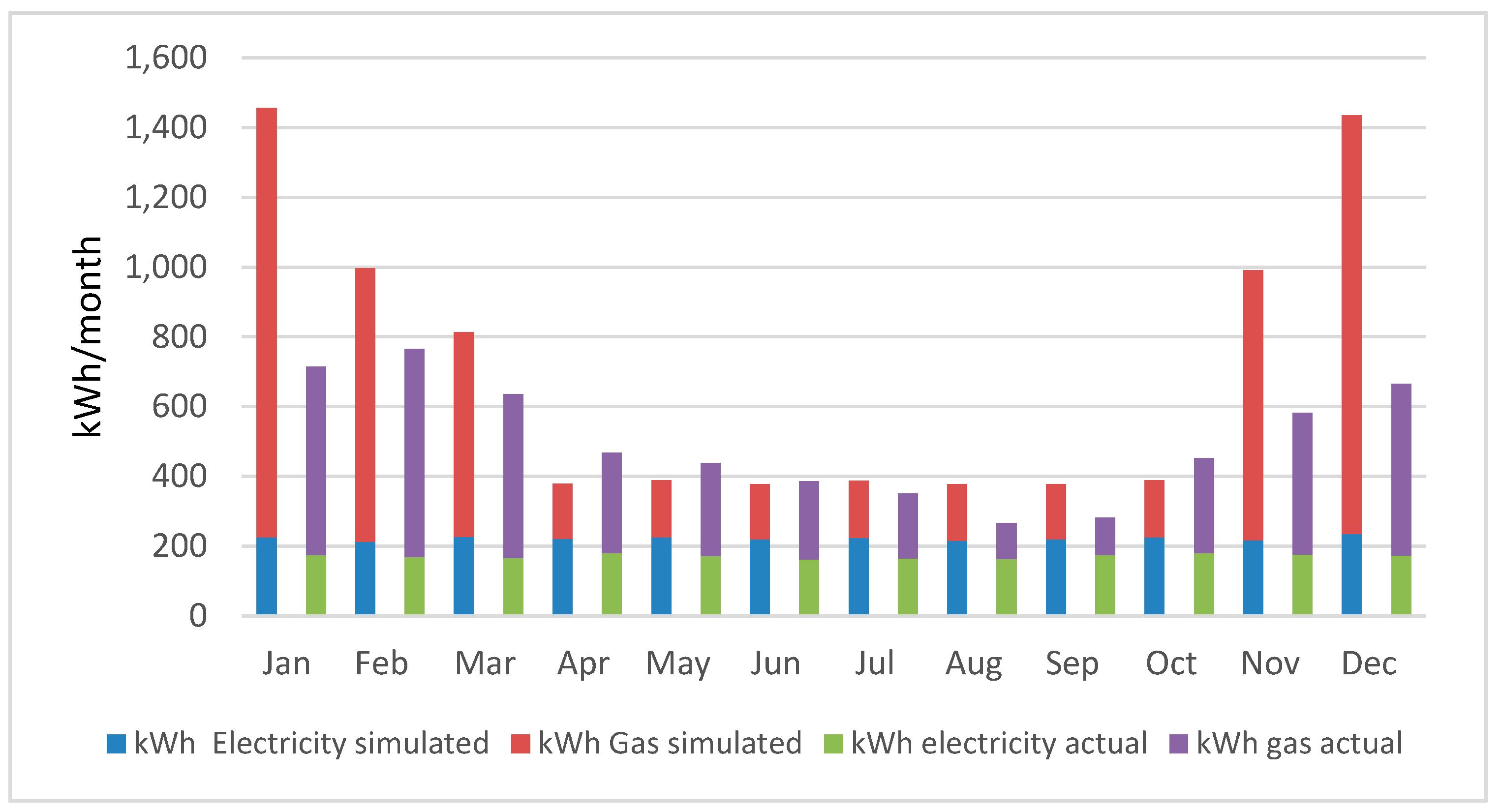
According to the average user profile defined in the Methodology, the heating is used for 59.5 h per week from November to March, which equals 1358 h per year. During these hours, the heating systems are available, but are not necessarily being used at full capacity. In Figure 5, the results of the simulation for building A (disaggregated by energy uses and sources) are depicted, taking into account this heating-user profile. The consumption of illumination and electrical appliances (there is a presumption of continued occupancy) is almost constant throughout the year. Likewise, the consumption for DHW varies little throughout the year, although the data has a slight U-shape owing to the different water-inlet temperature throughout the year. Electricity consumption represents 32% of the total annual energy consumption and DHW 23%. Heating consumption is the most significant, accounting for 45% of total annual energy consumption, but it presents significant monthly variations, accounting for up to 73% of total consumption in December and January.
4.3. Validation of Results
4.3.1. Simulation-Model Validation
Since actual energy consumption data are available, the simulation model was validated by comparing simulated and actual data. Table 7 compares annual simulated energy consumption versus actual energy consumption. In building A, simulated consumption is 39% higher than actual consumption (6003 kWh/year). This difference occurs for both electricity (30% higher) and gas (44% higher). The most noticeable difference between simulated and measured consumptions can be found in relation to heating, where the difference is as high as 131%.
Upon examination of the monthly distribution of consumption depicted in Figure 5, we can note that the difference between actual and simulated consumption (excluding the winter months) is relatively low. This difference is greater in April and October when the simulation considers that the heating is turned off but actually it is on for some time during the coldest days. Therefore, the biggest difference between actual and estimated consumption is in relation to heating consumption during the winter months, from November to March. The lower the outside temperature, the greater this difference becomes.
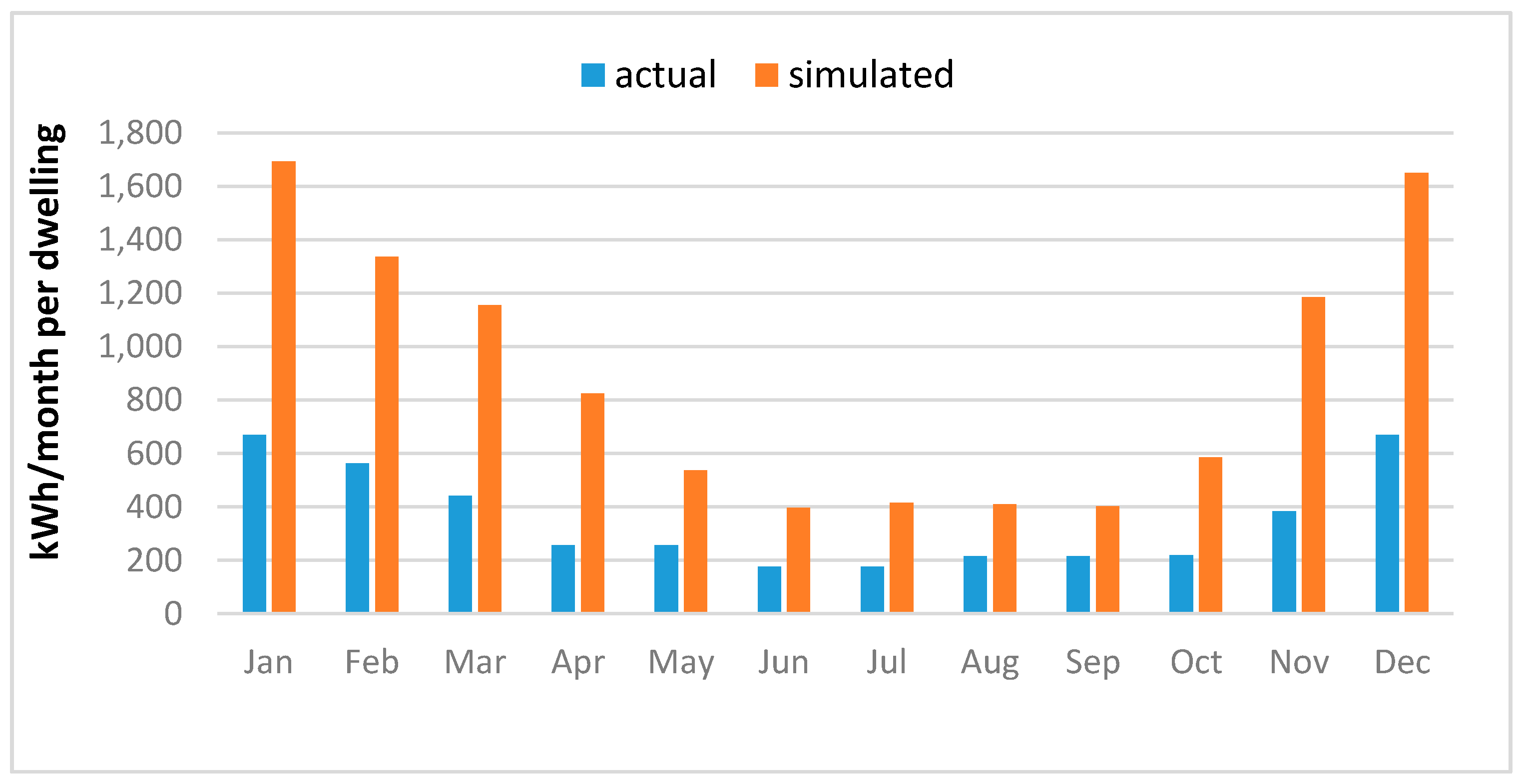
Similar trends were noted when we compared simulated and actual consumption for building B (see Table 8 and Figure 6). However, in this case, the difference between yearly simulated and measured consumption was 149%—even higher than in building A. The main source of difference is again the heating consumption.
Silva and Ghisi [67] found differences of 43.5% between simulation and actual consumptions in an uncertainty analysis of the behaviour of generic users (not necessarily vulnerable users) and included additional physical parameters. The difference noted in their study of 43.5% is similar to that noted for building A in our study. We may conclude that the model requires adjustments be made to the input parameters to accurately describe the energy performance of social housing. A sensitivity analysis for the variables used in the model follows here.
4.3.2. Sensitivity Analysis for the Parameters of the Simulation Model
Reasons for the significant differences between simulated and actual results can be ascertained. Some of them are related to the constraints of using a software-simulation tool (geometry, climatic model, etc.). Others may be explained by inaccuracy in relation to the hypothesised data for unknown variables such as air tightness. In addition, household structure and user profiles are difficult to simulate. A sensitivity analysis for the modelling design parameters is proposed here:
- Modelling of geometries and volume loses precision when flexibility, speed and ease of use of the design software are prioritised. One of the disadvantages is the inability to introduce curved geometric shapes, or include the consumption of certain specific equipment besides HVAC, as Herrando et al. [68] has noted in a previous study on tertiary buildings.
- Air tightness, which significantly affects the consumption of heating [69], is unknown and has not been measured accurately. In addition, it is also dependent on the user factor—e.g., different and variable ventilation times in each dwelling. Moreover, the effect of natural ventilation on heating consumption differs according to the thermal inertia of the building [70]. To better study the effect of air changes per hour, 1, 1.5 and 2 ac/h were simulated for building B in winter. In Figure 7, it can be observed that shifting from 1 to 1.5 ac/h requires an additional 16% in heating power whereas for a shift from 1.5 to 2 ac/h the increase is 12%. A higher increase in total energy demand was noted during the coldest months.
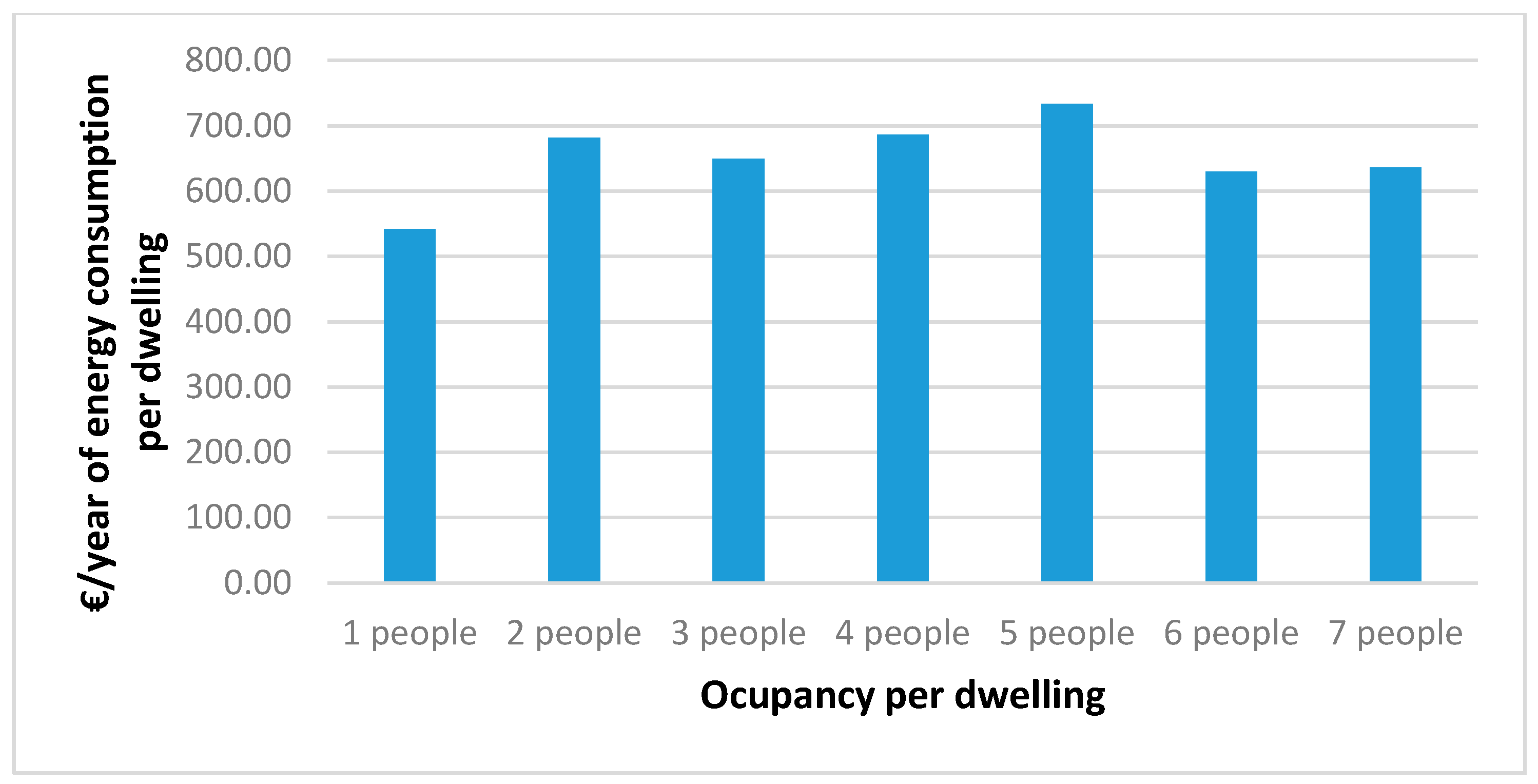
- Energy consumption was relatively unaffected by occupancy above two members, but this influence was noted as significant for one-person households. This significance is clear from the actual-to-simulated consumption differences for building B throughout the year: over one-third of the dwellings in this building are occupied by just one person. As shown in Figure 8, for occupancy levels above two people, significant variations in the annual consumption per dwelling are not observed, and thus we can posit that this variable is not particularly relevant.
- Materials and transmittance data are usually directly taken from technical data sheets and drawings of buildings. However, in this study, we found that these values can vary significantly with respect to the actual measured values, owing to documentation errors, the quality of the execution of the work, or simply owing to material deterioration. In the case of building B, the difference between the theoretical thermal transmittance of the outer wall (0.5 W/m2K) and the actual value (0.91 W/m2K) was 0.4 W/m2K. Measured values have been used in the simulation.
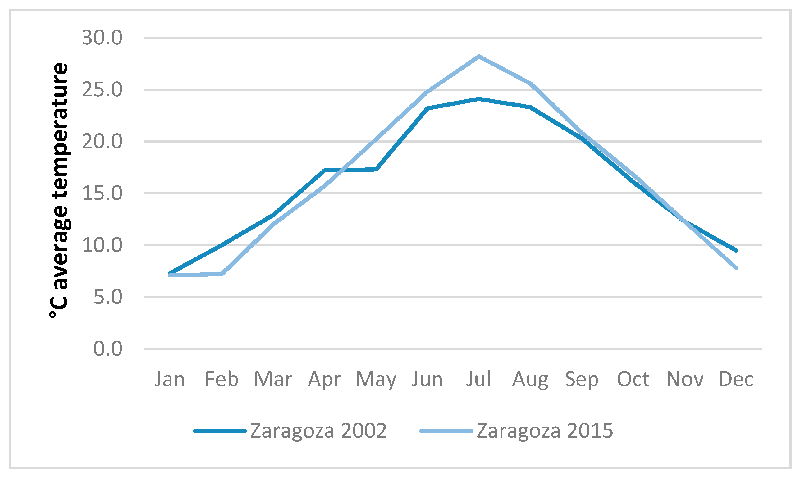
- The climate model in the simulation depends on the climatic zone, and does not take into account local or annual variations. The climate data used by the simulation software are based on hourly values for the year 2002, compiled in a .epw format file [37], but the year of the analysis is 2015. To illustrate the margin of error for the climate, Figure 9 depicts the difference in average temperatures between these two years (2002 and 2015) in Zaragoza.
In general, 2015 was 0.4 °C warmer than 2002. However, the temperature distribution indicates that there was an average increase of 2.1 °C in summer 2015 and a decrease of 1.1 °C in winter 2015, resulting in greater thermal discomfort in summer, and higher consumption of heating in winter; with respect to the data obtained in the simulation, this is important because the difference between these data and the actual consumption data is very significant. These deviations would result in a 7.7% increase in the heating consumption obtained by means of simulation.
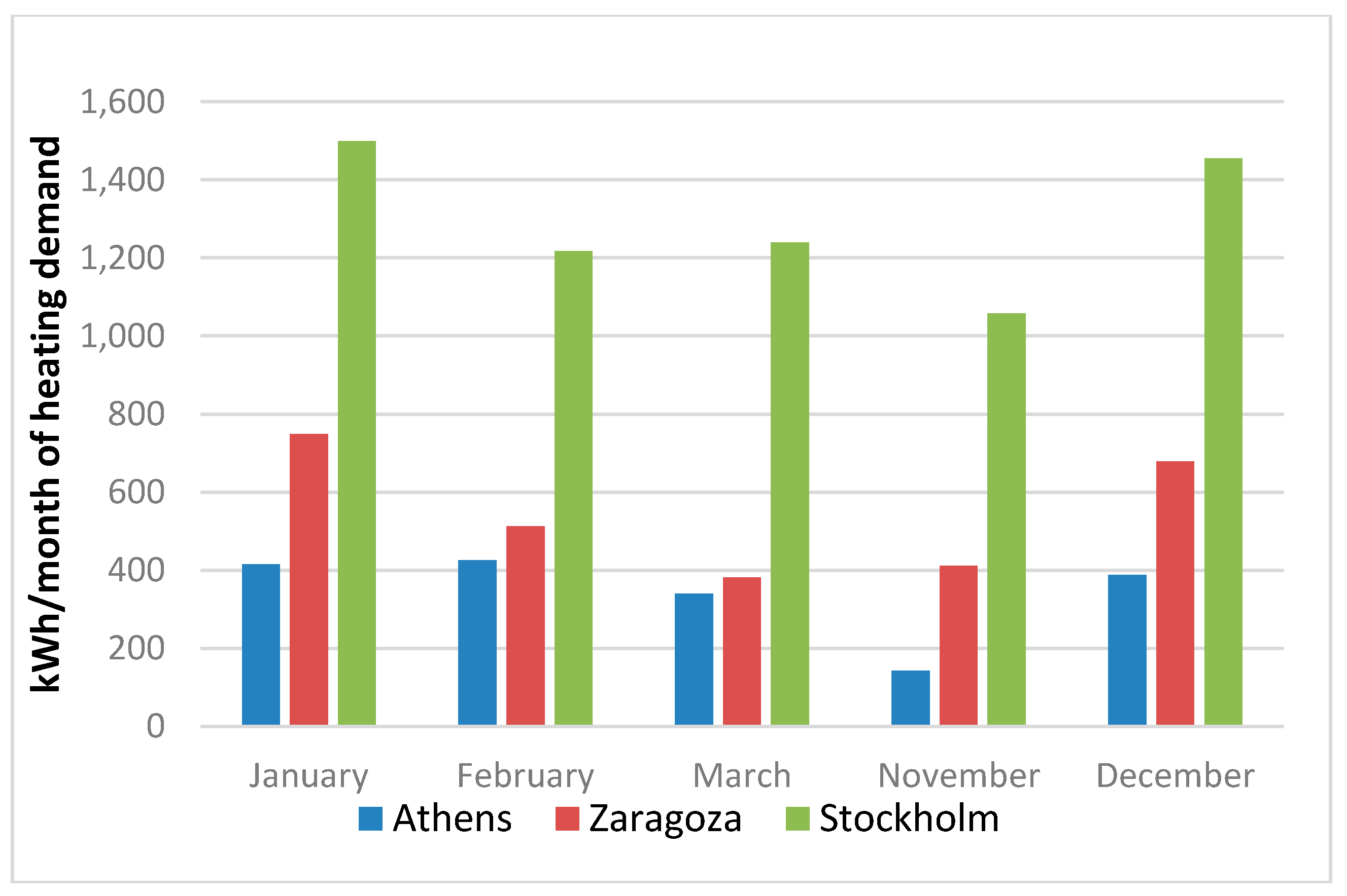
To illustrate dependence on a specific type of climate, a type “A” dwelling was simulated in three different European climates. The first dwelling is located in Athens (Greece), where there is a warm Mediterranean climate; the second is located in Zaragoza (Spain), where a Continental Mediterranean climate exists; and the last dwelling is located in Stockholm (Sweden), where there is a Continental Northern Atlantic climate. Figure 10 indicates the heating demand in kWh for the core winter months in the year of reference (2002). Keeping the user profiles and the other parameters constant, it can be observed that the house in Athens requires 37% less heating than the house in Zaragoza; during the same period in Stockholm, 136% more heating is needed than in Zaragoza. This difference is greater in the coldest months than in the mildest ones.
- The household structure is another relevant factor. Households with children or elderly people, who have higher care requirements and spend longer at home, would imply higher energy consumption [71]. In the case under study, 60% of the households are households with children (mainly living in building A), and 45% of those families surveyed report elderly people living at home. However, the level of influence of this factor could not be calculated in the present study since households with a higher number of residents are usually larger in size, and size seems to be of more relevance to increased energy consumption than occupancy.
The aforementioned variables that affect energy-simulation results do not explain by themselves the significant differences between simulation and actual consumption. New simulations with adjusted parameters were run and the main differences persisted. A more significant factor must thus explain those differences.
4.3.3. Adjustment and Fine-Tuning of model User Profiles
The reasons for the deviations may be related to the uses and habits of the tenants in social housing, many of whom are at risk of energy poverty. These consumption patterns of energy-poor households are similar across Europe, and this has been noted by Kolokotsa and Santamouris [72]. The economic constraints placed on these households reduce the residents’ energy use, affecting the conditions of comfort negatively.
These economic limitations primarily affect the target setpoint temperature values for comfort and the hours the heating equipment is operated. The greatest differences in heating have been attributed to the heating profiles declared by the residents (which were then applied in simulations): these differ significantly from the actual, measured profiles. The interviews demonstrate that tenants usually apply acceptable set-point temperature values but reduce the number of hours of heating, or the number of heated rooms, which eventually reduces the comfort conditions. The higher cost of electricity-powered heating in building B makes this building’s residents even more vulnerable than those of building A, and this explains the higher difference between simulated and real consumptions in building B when compared to building A.
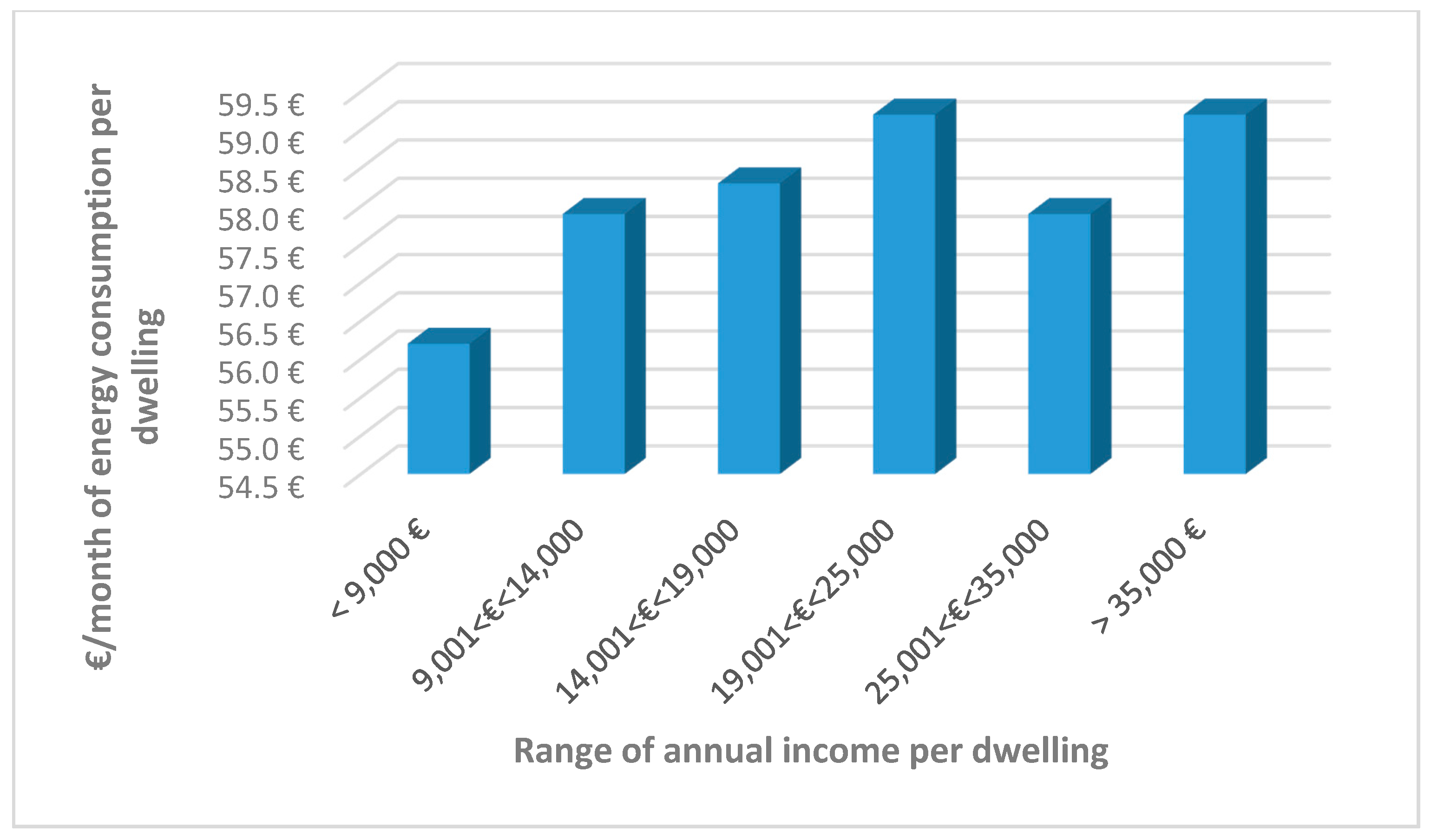
Figure 11 shows how the monthly energy expenditure per household increases with the level of income to a point where the energy needs are supposed to be fully covered and there is not any additional energy consumption.
According to the simulations carried out, to achieve some convergence between the simulated heating consumption and the actual consumption, it would be necessary to adjust the annual hours of heating from 1405 to 564 h in the case of building A and to 445 h in the case of building B. This adjustment would mean setting 3.5 daily hours for heating in building A and less than three daily hours for building B in winter. However, common practice is not to reduce the overall heating hours but rather to keep smaller areas warm for longer. This result is in line with the observations of Santamouris et al. [73], who studied a sample of 50 households in Athens.
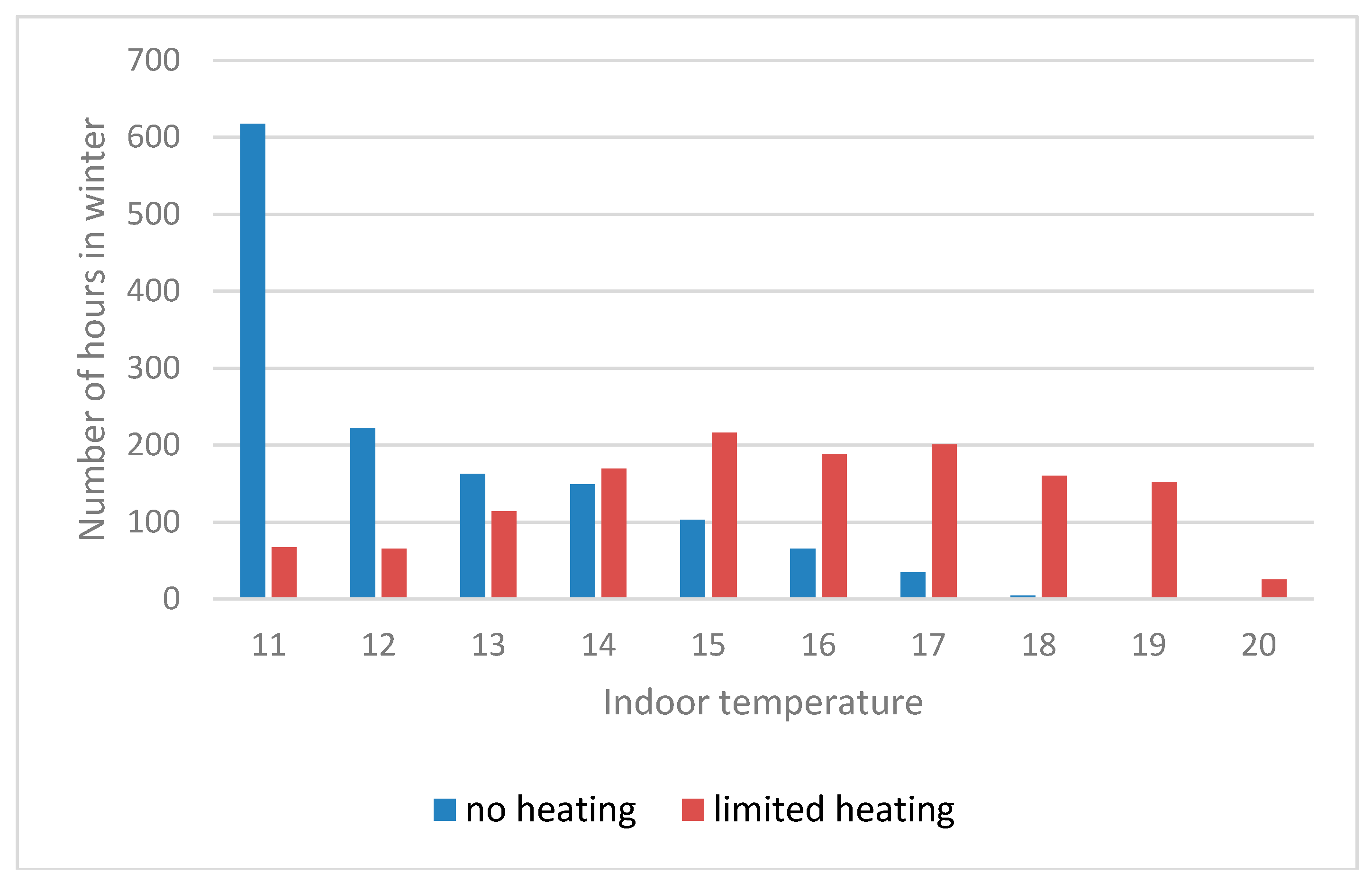
Energy poverty affects thermal comfort in dwellings; this is clear. Figure 11 allows for the straightforward identification of the simulated comfort level. It demonstrates the number of hours for which a home in building A is maintained at a given temperature during the period 1 November to 31 March for both situations: with heating and without heating (limited to the actual consumption).
Figure 12 shows that, without heating, the indoor temperature is not higher than 14 °C 75% of the time. When the heating system in the houses is on, cold hours are reduced to 33% of the winter season but the temperature hardly reaches 20 °C (considered to be the temperature required to achieve thermal comfort). In summary, according to the measured data for the dwellings under study, the use of the heating system increases the indoor temperature but the dwellings do not reach the desired comfort level.
5. Conclusions
This paper corroborates the hypothesis that the main cause of energy poverty is a level of income insufficient to satisfy the primary energy needs of a household. However, for a given income level, there are other factors that contribute to increase the impact of energy poverty on households. Building characteristics are not necessarily the most relevant factors when it comes to energy poverty. The structure of households and the behaviour of residents also play an important role. The cost of energy is considered relevant, mainly for electricity. In addition, the supply-contract typology does not always enable the optimisation of tariffs to the actual needs of social housing tenants.
Based on this analysis of the energy consumption and the household behaviour in situations of energy poverty, it was observed that users make proper use of the facilities, practise efficient ventilation and disconnect the systems when they are not in use, or when they are not at home. The greatest expenditure of energy was on heating, which social housing tenants underused; thus, they are prevented from achieving minimum indoor comfort conditions of 20 °C.
The optimisation of contracts and energy tariffs, as well as the diversification and shift to more affordable energy sources for heating, as opposed to Joule heating, are the most straightforward recommendations for those living in social housing to palliate energy poverty. Dwellings with only an electricity supply have energy costs which are almost double that of homes using natural gas for DHW and heating, even in cases of buildings which are more energy efficient.
Energy poverty translates into lower levels of thermal comfort in the affected households. The difference between pre-determined and actual user profiles and habits is the main cause of the deviations between the actual and the simulated energy consumption in social housing. We suggest that the standard comfort temperatures (21 °C) is not correct for energy-vulnerable households. In the analysed households, the simulated heating schedule should be significantly reduced, to between 3 and 3.5 h of heating service per day in winter season, to match the actual heating consumption in the social housing sample under study.
It should be noted that any improvement in the building envelope would not fully translate into real energy savings, but it would contribute to improve the thermal comfort conditions of those living in social housing, and thus would have a positive social impact quite separate from economic savings. The main reason is that those living in households suffering from energy poverty already live below standard comfort conditions: improvements to energy performance are likely to improve the residents’ thermal comfort by bringing the temperature closer to the standard level rather than driving down their already-low energy expenditure.
The obtained results contribute to improve the simulation tools for measuring energy poverty and social housing. These results can also be used to support decision-making processes concerning the management of household energy poverty in social housing—e.g., in relation to building refurbishment, maintenance, and energy-supply management.
Acknowledgments
The authors want to express their gratitude to the CATEDRA ZARAGOZA VIVIENDA—University of Zaragoza—within the framework of the 2014 call for research grants, approved on 4 December 2014, and funded by the Government of Aragón.
Author Contributions
All the authors collaborated in the study and in the paper elaboration. In particular, Juan Aranda designed the study, established the parameters to be assessed, carried out the data analysis. Ignacio Zabalza-Bribián is an expert in the sustainable building field and his contribution was specially focused on the dwelling characterization. He is also the corresponding author. Eva Llera-Sastresa’s contribution is specially focused on the characterization of the energy user behaviour. Sabina Scarpellini is an expert in energy poverty in households and her contribution is specially focused on the theoretical background of the study. Finally, Alfonso Alcalde performed the simulations and the energy audits under the supervision of Ignacio Zabalza and Juan Aranda.
Conflicts of Interest
The authors declare no conflict of interest. The founding sponsors had no role in the design of the study; in the collection, analyses, or interpretation of data; in the writing of the manuscript, and in the decision to publish the results.
References
- European Economic and Social Committee. For Coordinated European Measures to Prevent and Combat Energy Poverty; EESE: Bruxelles, Belgium, 2013. [Google Scholar]
- European Commission. Regulation of the European Parliament and of the Council on the Internal Market for Electricity; European Commission: Brussels, Belgium, 2016. [Google Scholar]
- Tirado Herrero, S.; Bouzarovski, S. Energy Transitions and Regional Inequalities in Energy Poverty Trends: Exploring the EU Energy Divide. Available online: https://ssrn.com/abstract=2537067 (accessed on 15 June 2017).
- Bouzarovski, S. Energy Poverty in the EU: A Review of the Evidence. Available online: http://citeseerx.ist.psu.edu/viewdoc/download?doi=10.1.1.593.7020&rep=rep1&type=pdf (accessed on 12 July 2017).
- Moore, R. Definitions of fuel poverty: Implications for policy. Energy Policy 2012, 49, 19–26. [Google Scholar] [CrossRef]
- International Energy Agency. Energy for All: Financing Access for the Poor (Special Early Excerpt of the World Energy Outlook 2011); IEA: Paris, France, 2011; 52p. [Google Scholar]
- Herrero Tirado, S.; López Fernández, J.L. Pobreza Energética en España. Potencial de Generación de empleo derivado de la rehabilitación energética de viviendas. Available online: http://www.niunhogarsinenergia.org/panel/uploads/documentos/estudio%20de%20pobreza%20energetica%20en%20espana%202012.pdf (accessed on 3 July 2017).
- Scarpellini, S.; Rivera-Torres, P.; Suarez-Perales, I.; Aranda-Uson, A. Analysis of energy poverty intensity from the perspective of the regional administration: Empirical evidence from households in southern Europe. Energy Policy 2015, 86, 729–738. [Google Scholar] [CrossRef]
- Hills, J. Getting the Measure of Fuel Poverty-Final Report of the Fuel Poverty Review; Summary Recommendation; Centre for the Analysis of Social Exclusion: London, UK, 2012. [Google Scholar]
- Teres-Zubiaga, J.; Martin, K.; Erkoreka, A.; Sala, J.M. Field assessment of thermal behaviour of social housing apartments in Bilbao, Northern Spain. Energy Build. 2013, 67, 118–135. [Google Scholar] [CrossRef]
- Santamouris, M.; Kapsis, K.; Korres, D.; Livada, I.; Pavlou, C.; Assimakopoulos, M.N. On the relation between the energy and social characteristics of the residential sector. Energy Build. 2007, 39, 893–905. [Google Scholar] [CrossRef]
- Rudge, J. Developing a Methodology to Evaluate the Outcome of Investment in Affordable Warmth: A Report to the Eaga Charitable Trust; Eaga Charitable Trust: Kendal, UK, 2001. [Google Scholar]
- Al-Azri, N.A. Development of a typical meteorological year based on dry bulb temperature and dew point for passive cooling applications. Energy Sustain. Dev. 2016, 33, 61–74. [Google Scholar] [CrossRef]
- Grevisse, F.; Brynart, M. Energy poverty in Europe: Towards a more global understanding. Eur. Counc. Energy Effic. Econ. 2011, 71, 537–549. [Google Scholar]
- Boardman, B. Fuel Poverty: From Cold Homes to Affordable Warmth; Belhaven Press: London, UK, 1991. [Google Scholar]
- Taylor, L. Fuel Poverty: From Cold Homes to Affordable Warmth. Energy Policy 1993, 21, 1071–1072. [Google Scholar] [CrossRef]
- Liddell, C.; Morris, C.; McKenzie, S.J.P.; Rae, G. Measuring and monitoring fuel poverty in the UK: National and regional perspectives. Energy Policy 2012, 49, 27–32. [Google Scholar] [CrossRef]
- Sovacool, B.K. The political economy of energy poverty: A review of key challenges. Energy Sustain. Dev. 2012, 16, 272–282. [Google Scholar] [CrossRef]
- Esmaeilimoakher, P.; Urmee, T.; Pryor, T.; Baverstock, G. Identifying the determinants of residential electricity consumption for social housing in Perth, Western Australia. Energy Build. 2016, 133, 403–413. [Google Scholar] [CrossRef]
- Jones, R.V.; Fuertes, A.; Boomsma, C.; Pahl, S. Space heating preferences in UK social housing: A socio-technical household survey combined with building audits. Energy Build. 2015, 127, 382–398. [Google Scholar] [CrossRef]
- Elsharkawy, H.; Rutherford, P. Retrofitting social housing in the UK: Home energy use and performance in a pre-Community Energy Saving Programme (CESP). Energy Build. 2015, 88, 25–33. [Google Scholar] [CrossRef]
- Filippidou, F.; Nieboer, N.; Visscher, H. Energy efficiency measures implemented in the Dutch non-profit housing sector. Energy Build. 2016, 132, 107–116. [Google Scholar] [CrossRef]
- AlFaris, F.; Juaidi, A.; Manzano-Agugliaro, F. Energy retrofit strategies for housing sector in the arid climate. Energy Build. 2016, 131, 158–171. [Google Scholar] [CrossRef]
- Pombo, O.; Allacker, K.; Rivela, B.; Neila, J. Sustainability assessment of energy saving measures: A multi-criteria approach for residential buildings retrofitting—A case study of the Spanish housing stock. Energy Build. 2016, 116, 384–394. [Google Scholar] [CrossRef] [Green Version]
- Ben, H.; Steemers, K. Energy retrofit and occupant behaviour in protected housing: A case study of the Brunswick Centre in London. Energy Build. 2014, 80, 120–130. [Google Scholar] [CrossRef]
- European Commission. Energy Poverty and Vulnerable Consumers in the Energy Sector across the EU: Analysis of Policies and Measures; European Commission: Brussels, Belgium, 2015. [Google Scholar]
- Li, K.; Lloyd, B.; Liang, X.J.; Wei, Y.M. Energy poor or fuel poor: What are the differences? Energy Policy 2014, 68, 476–481. [Google Scholar] [CrossRef]
- Tronchin, L.; Fabbri, K. Energy performance building evaluation in Mediterranean countries: Comparison between software simulations and operating rating simulation. Energy Build. 2008, 40, 1176–1187. [Google Scholar] [CrossRef]
- Wang, H.; Zhai, Z. Advances in building simulation and computational techniques: A review between 1987 and 2014. Energy Build. 2016, 128, 319–335. [Google Scholar] [CrossRef]
- Escandón, R.; Suárez, R.; Sendra, J.J. On the assessment of the energy performance and environmental behaviour of social housing stock for the adjustment between simulated and measured data: The case of mild winters in the Mediterranean climate of southern Europe. Energy Build. 2017, 152, 418–433. [Google Scholar] [CrossRef]
- Aranda, J.; Zabalza, I.; Conserva, A.; Millan, G. Analysis of Energy Efficiency Measures and Retrofitting Solutions for Social Housing Buildings in Spain as a way to mitigate Energy Poverty. Sustainability 2017, 9, 1869. [Google Scholar] [CrossRef]
- Sdei, A.; Gloriant, F.; Tittelein, P.; Lassue, S.; Hanna, P.; Beslay, C.; Gournet, R.; McEvoy, M. Social housing retrofit strategies in England and France: A parametric and behavioural analysis. Energy Res. Soc. Sci. 2015, 10, 62–71. [Google Scholar] [CrossRef]
- Ramos, N.M.M.; Almeida, R.M.S.F.; Simões, M.L.; Pereira, P.F. Knowledge discovery of indoor environment patterns in mild climate countries based on data mining applied to in-situ measurements. Sustain. Cities Soc. 2017, 30, 37–48. [Google Scholar] [CrossRef]
- Nguene, G.; Fragnire, E.; Kanala, R.; Lavigne, D.; Moresino, F. SOCIO-MARKAL: Integrating energy consumption behavioral changes in the technological optimization framework. Energy Sustain. Dev. 2011, 15, 73–83. [Google Scholar] [CrossRef]
- De Lieto Vollaro, R.; Guattari, C.; Evangelisti, L.; Battista, G.; Carnielo, E.; Gori, P. Building energy performance analysis: A case study. Energy Build. 2015, 87, 87–94. [Google Scholar] [CrossRef]
- Webb, J.; Hawkey, D.; McCrone, D.; Tingey, M. House, home and transforming energy in a cold climate. Fam. Relatsh. Soc. 2016, 5, 411–429. [Google Scholar] [CrossRef]
- DesignBuilder Software Ltd. DesignBuilder 4.0 User’s Manual 2014; DesignBuilder Software Ltd.: Stroud, UK, 2014. [Google Scholar]
- Mirakhorli, A.; Dong, B. Occupancy behavior based model predictive control for building indoor climate: A critical review. Energy Build. 2016, 129, 499–513. [Google Scholar] [CrossRef]
- Hamza, N.; Zi, Q.; Stein, O. User behaviours and preferences for low carbon homes: Lessons for predicting energy demand. In Proceedings of the 14th International Conference of IBPSA-Building Simulation 2015 (BS 2015), Hyderabad, India, 7–9 December 2015. [Google Scholar]
- Eastaway, M.P.; Varo, I.S.M. The Tenure Imbalance in Spain: The Need for Social Housing Policy. Urban Stud. 2002, 39, 283–295. [Google Scholar] [CrossRef]
- Real Decreto 2429/1979. BOE-A-1979-24866. Available online: https://www.boe.es/diario_boe/txt.php?id=BOE-A-1979-24866 (accessed on 10 February 2017).
- Azevedo, J.A.; Chapman, L.; Muller, C.L. Critique and suggested modifications of the degree days methodology to enable long-term electricity consumption assessments: A case study in Birmingham, UK. Meteorol. Appl. 2015, 22, 789–796. [Google Scholar] [CrossRef]
- AEMET (Agencia Estatal de Meteorología Ministerio de Agricultura y Pesca Alimentación y Medio Ambiente—Gobierno de España). Valores climatológicos Normales. Zaragoza Aeropuerto. Available online: http://www.aemet.es/es/serviciosclimaticos/datosclimatologicos/valoresclimatologicos?l=9434&k=arn (accessed on 5 October 2016).
- Ministerio de Fomento. Código técnico de la Edificación. Documento Básico HE Ahorro de Energía; Ministerio de Fomento: Madrid, Spain, 2013; pp. 1–70. [Google Scholar]
- Instituto Nacional de Estadística (INE). Encuesta de Condiciones de Vida 2015; INE: Madrid, Spain, 2015.
- Consulting AG. Mapa de distribución de los ingresos medios de las familias a nivel municipal en el territorio español; Consulting AG: Vienna, Austria, 2014. [Google Scholar]
- Macias, M.; Mateo, A.; Schuler, M.; Mitre, E.M. Application of night cooling concept to social housing design in dry hot climate. Energy Build. 2006, 38, 1104–1110. [Google Scholar] [CrossRef]
- Bouzarovski, S. Energy poverty in the European Union: Landscapes of vulnerability. Wiley Interdiscip. Rev. Energy Environ. 2014, 3, 276–289. [Google Scholar] [CrossRef]
- Alkon, M.; Harish, S.P.; Urpelainen, J. Household energy access and expenditure in developing countries: Evidence from India, 1987–2010. Energy Sustain. Dev. 2016, 35, 25–34. [Google Scholar] [CrossRef]
- Wu, M.H.; Ng, T.S.; Skitmore, M.R. Sustainable building envelope design by considering energy cost and occupant satisfaction. Energy Sustain. Dev. 2016, 31, 118–129. [Google Scholar] [CrossRef]
- Institute for Energy Diversification and Saving (IDAE). Project Sech-Spahousec, Analysis of the Energetic Consumption of the Residential Sector in Spain (Proyecto Sech-Spahousec, Análisis del Consumo Energético del Sector Residencial en España); IDAE: Madrid, Spain, 2016. [Google Scholar]
- Scarpellini, S.; Sanz Hernández, M.A.; Llera-Sastresa, E.; Aranda, J.A.; López Rodríguez, M.E. The mediating role of social workers in the implementation of regional policies targeting energy poverty. Energy Policy 2017, 106, 367–375. [Google Scholar] [CrossRef]
- Karlin, B.; Davis, N.; Sanguinetti, A.; Gamble, K.; Kirkby, D.; Stokols, D. Dimensions of Conservation: Exploring Differences among Energy Behaviors. Environ. Behav. 2012, 46, 423–452. [Google Scholar] [CrossRef]
- Iwata, K.; Katayama, H.; Arimura, T.H. Do households misperceive the benefits of energy-saving actions? Evidence from a Japanese household survey. Energy Sustain. Dev. 2015, 25, 27–33. [Google Scholar] [CrossRef]
- Chester, L. Energy Impoverishment: Addressing Capitalism’s New Driver of Inequality. J. Econ. Issues 2014, 48, 395–404. [Google Scholar] [CrossRef]
- Bradshaw, J.L.; Bou-Zeid, E.; Harris, R.H. Greenhouse gas mitigation benefits and cost-effectiveness of weatherization treatments for low-income, American, urban housing stocks. Energy Build. 2016, 128, 911–920. [Google Scholar] [CrossRef]
- Treiber, M.U.; Grimsby, L.K.; Aune, J.B. Reducing energy poverty through increasing choice of fuels and stoves in Kenya: Complementing the multiple fuel model. Energy Sustain. Dev. 2015, 27, 54–62. [Google Scholar] [CrossRef]
- Santamouris, M. Innovating to zero the building sector in Europe: Minimising the energy consumption, eradication of the energy poverty and mitigating the local climate change. Sol. Energy 2016, 128, 61–94. [Google Scholar] [CrossRef]
- Teli, D.; Dimitriou, T.; James, P.A.B.; Bahaj, A.S.; Ellison, L.; Waggott, A. Fuel poverty-induced prebound effect’ in achieving the anticipated carbon savings from social housing retrofit. Build. Serv. Eng. Res. Technol. 2016, 37, 176–193. [Google Scholar] [CrossRef]
- Ormandy, D.; Ezratty, V. Thermal discomfort and health: Protecting the susceptible from excess cold and excess heat in housing. Adv. Build. Energy Res. 2015, 10, 84–98. [Google Scholar] [CrossRef]
- Schueftan, A.; Sommerhoff, J.; Gonzalez, A.D. Firewood demand and energy policy in south-central Chile. Energy Sustain. Dev. 2016, 33, 26–35. [Google Scholar] [CrossRef]
- Swan, W.; Ruddock, L.; Smith, L. Low carbon retrofit: Attitudes and readiness within the social housing sector. Eng. Constr. Archit. Manag. 2013, 20, 522–535. [Google Scholar] [CrossRef]
- Patterson, J.; Louise, J. Evaluation of a Regional Retrofit Programme to Upgrade Existing Housing Stock to Reduce Carbon Emissions, Fuel Poverty and Support the Local Supply Chain. Sustainability 2016, 8, 1261. [Google Scholar] [CrossRef]
- Altan, H.; Gasperini, N.; Moshaver, S.; Frattari, A. Redesigning terraced social housing in the UK for flexibility using building energy simulation with consideration of passive design. Sustainability 2015, 7, 5488–5507. [Google Scholar] [CrossRef]
- Real Decreto 235/2013. Available online: https://www.boe.es/buscar/act.php?id=BOE-A-2013-3904 (accessed on 5 May 2017).
- Ramos, N.M.M.; Almeida, R.M.S.F.; Curado, A.; Pereira, P.F.; Manuel, S.; Maia, J. Airtightness and ventilation in a mild climate country rehabilitated social housing buildings—What users want and what they get. Build. Environ. 2015, 92, 97–110. [Google Scholar] [CrossRef]
- Silva, A.S.; Ghisi, E. Uncertainty analysis of user behaviour and physical parameters in residential building performance simulation. Energy Build. 2014, 76, 381–391. [Google Scholar] [CrossRef]
- Herrando, M.; Cambra, D.; Navarro, M.; de la Cruz, L.; Millan, G.; Zabalza, I. Energy Performance Certification of Faculty Buildings in Spain: The gap between estimated and real energy consumption. Energy Convers. Manag. 2016, 125, 141–153. [Google Scholar] [CrossRef]
- Šadauskienė, J.; Paukštys, V.; Šeduikytė, L.; Banionis, K. Impact of Air Tightness on the Evaluation of Building Energy Performance in Lithuania. Energies 2014, 7, 4972–4987. [Google Scholar] [CrossRef]
- Sorgato, M.J.; Melo, A.P.; Lamberts, R. The effect of window opening ventilation control on residential building energy consumption. Energy Build. 2016, 133, 1–13. [Google Scholar] [CrossRef]
- Walker, G.; Brown, S.; Neven, L. Thermal comfort in care homes: Vulnerability, responsibility and “thermal care”. Build. Res. Inf. 2015, 3218, 1–14. [Google Scholar] [CrossRef]
- Kolokotsa, D.; Santamouris, M. Review of the indoor environmental quality and energy consumption studies for low income households in Europe. Sci. Total Environ. 2015, 536, 316–330. [Google Scholar] [CrossRef] [PubMed]
- Santamouris, M.; Alevizos, S.M.; Aslanoglou, L.; Mantzios, D.; Milonas, P.; Sarelli, I.; Karatasou, S.; Cartalis, K.; Paravantis, J.A. Freezing the poor—Indoor environmental quality in low and very low income households during the winter period in Athens. Energy Build. 2014, 70, 61–70. [Google Scholar] [CrossRef]
Figure 1.
Flow chart depicting the buildings’ energy performance methodology.

Figure 2.
Average monthly energy consumption (kWh/month) in the average dwelling of the analysed buildings A (left) and B (right).
Figure 2.
Average monthly energy consumption (kWh/month) in the average dwelling of the analysed buildings A (left) and B (right).
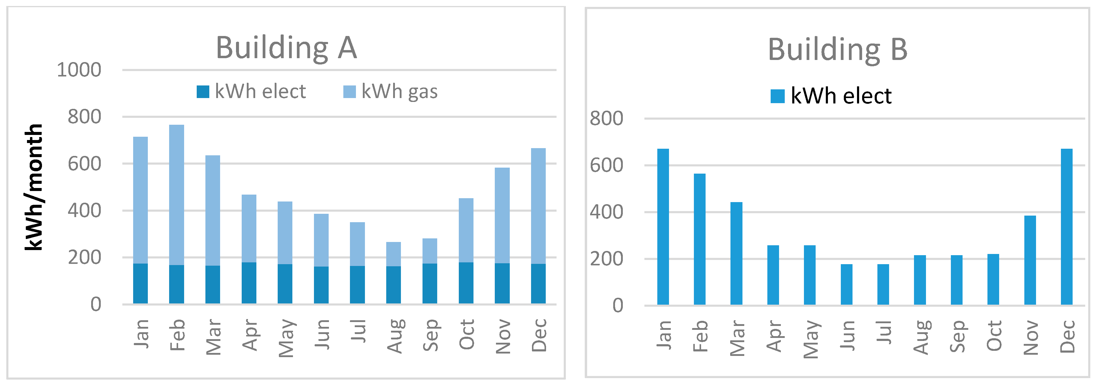
Figure 3.
Ratio of annual energy costs and annual income distributed by income level (€/year) of the households.
Figure 3.
Ratio of annual energy costs and annual income distributed by income level (€/year) of the households.

Figure 4.
3D model of: building A (left); and building B (right).
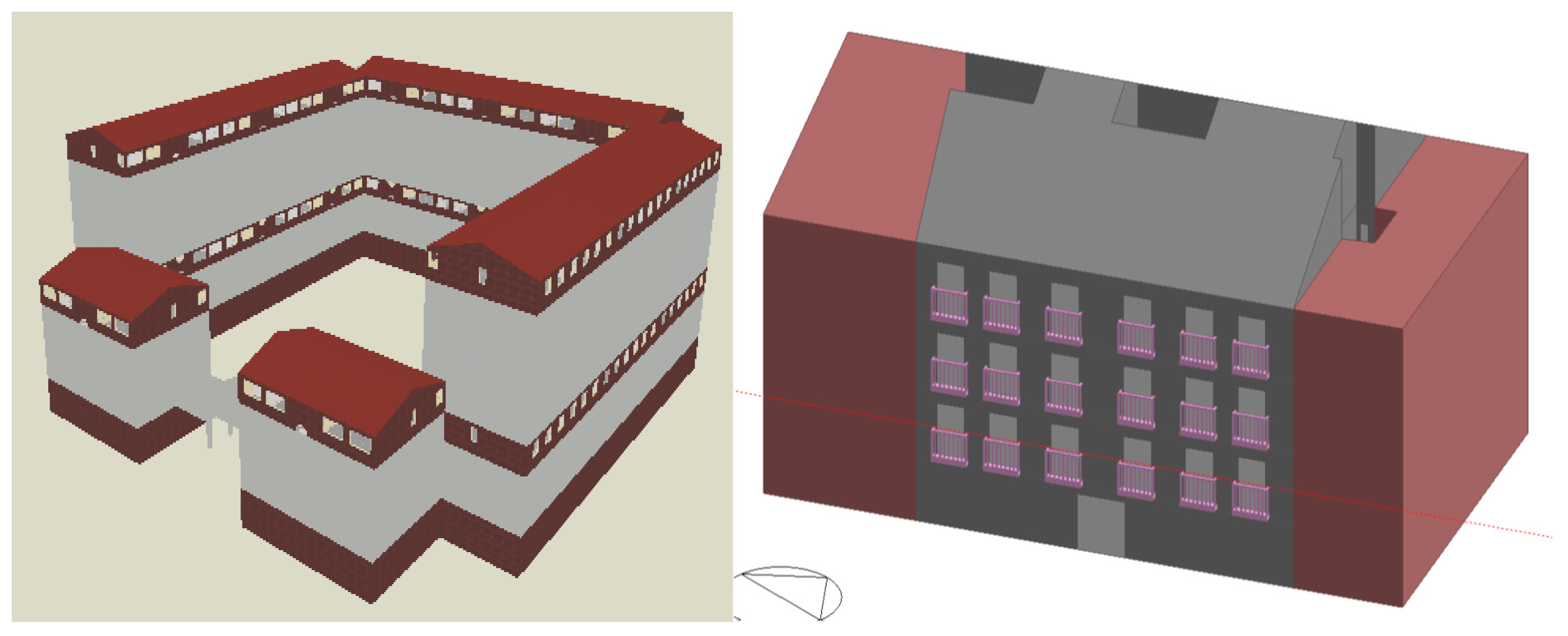
Figure 5.
Monthly average for simulated and actual final energy consumption (kWh/month) per dwelling in building A.
Figure 5.
Monthly average for simulated and actual final energy consumption (kWh/month) per dwelling in building A.

Figure 6.
Monthly average of simulated and actual final energy consumption (kWh/month) per dwelling in building B.
Figure 6.
Monthly average of simulated and actual final energy consumption (kWh/month) per dwelling in building B.

Figure 7.
Monthly heating demand (kWh per month) for several levels of air changes per hour for a dwelling in building B.
Figure 7.
Monthly heating demand (kWh per month) for several levels of air changes per hour for a dwelling in building B.

Figure 8.
Average annual energy cost per occupancy level (€/year): Building A.

Figure 9.
Average daily temperature in Zaragoza (°C) in the reference year 2002 and in year 2015.

Figure 10.
Heating demand (kWh per month) for a type-A dwelling in three different European climates.
Figure 10.
Heating demand (kWh per month) for a type-A dwelling in three different European climates.

Figure 11.
Monthly energy expenditure in €/month per household versus annual income levels: Building A.
Figure 11.
Monthly energy expenditure in €/month per household versus annual income levels: Building A.

Figure 12.
Number of hours and the indoor temperature for a dwelling in building A in winter, with and without heating (limited to actual figures of consumption).
Figure 12.
Number of hours and the indoor temperature for a dwelling in building A in winter, with and without heating (limited to actual figures of consumption).


Table 1.
Household information inquired.
| (1) Building characteristics | (2) Equipment characteristics |
| - Surface area | - Household equipment HVAC and DHW systems |
| - Envelope materials and quality | - Other energy-consuming elements |
| - Refurbishments undertaken to date | |
| (3) Energy supply and consumption per year | (4) Household structure and consumption habits |
| - Type of energy-supply contract (utilities) | - Frequency of equipment use |
| - Energy consumption invoiced per year and type of energy invoiced | - Intensity of equipment use |
| - Number of residents | |
| - Employment situation of each resident | |
| - Annual net income |
Table 2.
General data of the buildings and residents.
| Building Data | Building A | Building B |
|---|---|---|
| Number of dwellings | 160 | 12 |
| Number of blocks | 11 | 1 |
| Build year | 1988 | 1988 |
| Orientation | All | N-S |
| Sample of dwellings/total number of dwellings | 36/160 | 8/12 |
| Average dwelling size (m2) | 68.5 | 55 |
| Number of floors on ground level | 8 | 3 |
| Useable surface on each floor (m2) | 1644 | 220 |
| Average number of occupants per dwelling | 3.7 | 2.8 |
| Surface area per occupant (m2/person) | 18.5 | 28.5 |
| Building refurbishment | No | partial |
| Other buildings surrounding the building | No | East and West |
Table 3.
Comparison of thermal-transmittance measurements of various enclosing areas of buildings A, B, B renewed and value required by current regulations CTE DB-HE1, in W/m2K.
Table 3.
Comparison of thermal-transmittance measurements of various enclosing areas of buildings A, B, B renewed and value required by current regulations CTE DB-HE1, in W/m2K.
| Type of Enclosure | Thermal Transmittance (W/m2K) | |||
|---|---|---|---|---|
| Building A | Building B | Building B, Renewed | CTE DB-HE1 | |
| External walls | 0.71 | 0.5 | 0.27 | 0.6 |
| Internal walls | 2.44 | 0.47 | 0.47 | 0.6 |
| Bottom floor | 1.12 | 0.5 | 0.33 | 0.4 |
| Roof | 0.51 | 1.18 | 0.19 | 0.4 |
| Windows (glazing type) | 5.7 (single glazing 6 mm) | 3.17 (double glazing 4-6-4) | 3.17 (double glazing 4-6-4) | 2.7 (-) |
Table 4.
Average socio-economic characteristics of households in Buildings A and B.
| Household Average Data | Building A | Building B |
|---|---|---|
| Average annual income (€/household) | €10,471 | €11,663 |
| Number of employed people per household | 0.7 | 0.4 |
| Number of children per household | 1.3 | 0.8 |
| Number of retired people per household | 0.6 | 0.9 |
Table 5.
Average actual energy consumption and cost ratios of households in buildings A and B.
| Household Average Energy Data | Building A | Building B |
|---|---|---|
| Annual energy consumption per household (kWh/year housing) | 6003 | 4249 |
| Annual energy cost per household (€/year housing) | 642 | 779 |
| Annual energy consumption per surface (kWh/m2 year) | 87.6 | 77.5 |
| Annual energy cost per m2 (€/m2 year) | 9.37 | 14.1 |
| Real thermal transmittance of facades (W/m2K) | 0.71 | 0.91 |
| Contracted power per housing (kW) | 3.52 | 5.6 |
| Equivalent hours of electricity usage per household (h/year) | 592 | 712 |
| Average overall cost of energy consumed (€/kWh) | 0.11 | 0.20 |
| Income percentage dedicated to energy costs (%) | 6.1% | 6.7% |
Table 6.
Comparison between the electrical consumption and economic cost in a household of four people in the buildings analysed and in an average reference home.
Table 6.
Comparison between the electrical consumption and economic cost in a household of four people in the buildings analysed and in an average reference home.
| Household | Power (kW) | Electricity Consumption (kWh/year) | Cost (€/year) | Electricity Average Price (€/kWh) |
|---|---|---|---|---|
| Building A | 3.8 | 2020 | €435 | €0.22 |
| Building B | 5.6 | 3695 | €771 | €0.21 |
| Reference home in Spain [50] | 4.4 | 3900 | €826 | €0.21 |
Table 7.
Comparison of simulated and actual consumption in the average dwelling in building A, in kWh/year.
Table 7.
Comparison of simulated and actual consumption in the average dwelling in building A, in kWh/year.
| Energy Consumption | Simulated Consumption (kWh/year) | Actual Consumption (kWh/year) | Change (%) |
|---|---|---|---|
| Electricity | 2669 | 2056 | 30% |
| DHW + others | 1920 | 2309 | −17% |
| Heating | 3779 | 1638 | 131% |
| TOTAL | 8368 | 6003 | 39% |
Table 8.
Comparison of simulated and actual consumption in a dwelling of building B, in kWh/year.
| Energy Consumption | Simulated Consumption (kWh/year) | Real Consumption (kWh/year) | Change (%) |
|---|---|---|---|
| Others | 6604 | 2980 | 122% |
| Heating | 3994 | 1268 | 215% |
| TOTAL | 10,598 | 4249 | 149% |
© 2018 by the authors. Licensee MDPI, Basel, Switzerland. This article is an open access article distributed under the terms and conditions of the Creative Commons Attribution (CC BY) license (http://creativecommons.org/licenses/by/4.0/).
Share and Cite
MDPI and ACS Style
Aranda, J.; Zabalza, I.; Llera-Sastresa, E.; Scarpellini, S.; Alcalde, A. Building Energy Assessment and Computer Simulation Applied to Social Housing in Spain. Buildings 2018, 8, 11. https://doi.org/10.3390/buildings8010011
AMA Style
Aranda J, Zabalza I, Llera-Sastresa E, Scarpellini S, Alcalde A. Building Energy Assessment and Computer Simulation Applied to Social Housing in Spain. Buildings. 2018; 8(1):11. https://doi.org/10.3390/buildings8010011
Chicago/Turabian StyleAranda, Juan, Ignacio Zabalza, Eva Llera-Sastresa, Sabina Scarpellini, and Alfonso Alcalde. 2018. "Building Energy Assessment and Computer Simulation Applied to Social Housing in Spain" Buildings 8, no. 1: 11. https://doi.org/10.3390/buildings8010011
Note that from the first issue of 2016, this journal uses article numbers instead of page numbers. See further details here.