Housing Affordability in Metropolitan Areas. The Application of a Combination of the Ratio Income and Residual Income Approaches to Two Case Studies in Sicily, Italy


Department of Architecture, University of Palermo, Palermo 90128, Italy
Buildings 2017, 7(4), 95; https://doi.org/10.3390/buildings7040095
Submission received: 31 August 2017
/
Revised: 20 October 2017
/
Accepted: 23 October 2017
/
Published: 26 October 2017
(This article belongs to the Special Issue Real Estate Economics, Management and Investments)
Abstract
:Housing affordability problems have become more serious over the course of the last few decades and are now also affecting the middle-class, despite the fall in prices on the housing market. This study proposes a methodology to assess threshold-income as an index for measuring housing affordability by applying a combination of the ratio income and residual income approaches. The methodology is applied to two particular areas of Sicily in Italy as case studies consisting of medium-size metropolitan areas located in a less developed European region. The areas have been chosen on the basis of their different territorial structure: a polarized area that comprises a high-density city centre and a polynuclear urban region. The results are diversified for income level, as well as for town and urban zone, and allow us to compare the housing affordability problems between towns belonging to the same metropolitan area.
1. Introduction
Though metropolitan and post-metropolitan areas have different territorial structures in that the former comprises a high-density city centre with urban sprawl in its hinterlands, while the latter comprises a polynuclear urban region, in both areas, residential and economic activities are strongly interconnected with mobility and communication infrastructures, owing to continuous flows of people, commodities, information, capital, and investment. These flows follow dynamics that modify the economic and demographic relationships that generate the growth or decline of towns or metropolitan territories [1,2,3]. The relationships between towns may be classified as hierarchical-vertical relationships between the hierarchy levels or as network-horizontal relationships, which may form a synergic network when there is an alliance between similar towns to achieve economies of scale or a complementarity network when different economic sectors create a value chain connecting various towns. More often, mixed relationships are observed, the nature of which is partly hierarchical and partly network [4,5,6]. Each town contributes to the ‘external competitiveness’ of the metropolitan area to which it belongs against other urban regions in terms of its abilities to attract inhabitants, capital, and services, whilst at the same time facing the internal competitiveness within the very metropolitan area itself, according to its own demographic and economic ranking, which may attract more investment and migratory flows [7,8].
From the economic point of view, the traditional neoclassical analysis of the choice of place to live is based on the trade-off between housing price and transport costs under the income threshold [9,10]. Obviously, the choices also depend on many other factors such as cultural, aesthetical, ethical, etc., but, nevertheless, housing price remains an acceptable conventional proxy of location quality (e.g., environmental, urban, and district quality) and of technological and architectural housing features, even if all these other factors may have diverse intensity and are variously combined in correspondence with the same overall price. Choosing a housing location may significantly depend on, or be seriously constrained by, the comparison of available income for housing and market prices (purchase or rental): ‘housing affordability’ is, precisely, a concept for analysing housing problems and defining housing need.
This study proposes to test a methodology to assess housing affordability problems in metropolitan and post-metropolitan areas in which, however, an all-encompassing housing policy has to be designed. The proposed methodology is applied to two areas, one in north-western Sicily (NWS) and the other in south-eastern Sicily (SES), as examples of medium-size metropolitan areas that are located in a less developed European region. These areas have been chosen on the basis of their different territorial structure: a polarized area that comprises a high-density city centre and a polynuclear urban region.
Starting from the basic concept that housing affordability always represents a relationship between people and price, the study is based on the analysis of the territorial distribution of both inhabitants’ incomes and the local real estate market. In a metropolitan area, housing prices may vary considerably according to the location; for this reason, the analysis of local real estate has been considered an important step of the methodology because it will allow us to identify which areas or municipalities are affordable/unaffordable by each household type. The local housing market can be gathered by collecting the housing prices in the central and peripheral zones of each municipality of the two metropolitan areas.
The collected data on household incomes and local housing prices are the main inputs for the assessment of threshold-income (T_I) by both the ratio income and the residual income approaches. According to the literature [11,12], the results of the ratio income approach may actually provide some distorted descriptions of the ability to purchase a house in correspondence to low and very low-income households. Consequently, a combined income approach is applied, as some others suggest [11,12], to reduce the methodological weakness of the income ratio, and for assessing the combined threshold-incomes. The combined threshold-income is used, not only to determine how many households have housing affordability problems, but also to show which locations in the metropolitan areas are affordable/not affordable. The mapping, in conjunction with other indexes, may support the metropolitan and urban planning by which the current ‘form’ of urban areas could be transformed in order to prevent, or to mitigate, the social polarization and ghettoization that are related to housing affordability problems [13].
In order to achieve this aim, Section 2 defines the concept of housing affordability and compares the most commonly used approaches for the assessment of housing affordability. In Section 3, a methodology is developed by using a combination of the ratio income and residual income approaches. In Section 4, the case study is presented, followed by the application of the ratio income, residual income, and combined approaches to two metropolitan areas. Section 5 discusses the results. In Section 6, the potential further development of the study is presented.
2. Housing Affordability: Concept and Measure
The debate in the literature is primarily focused on the very meaning of the term ‘housing affordability’ and on how to measure it.
The term ‘housing affordability’ began to be used from the 1980s and may be defined in various ways, among which we can cite: housing affordability refers to the capacity of households to meet housing costs, while maintaining the ability to meet other basic costs of living [14]; a rent is affordable when it leaves the consumer with a socially acceptable standard of both housing and non-housing consumption after rent is paid [15]; a household is said to have a housing affordability problem when it pays more than a certain percentage of its income to obtain adequate and appropriate housing [16].
Beyond a simple definition, however, it is important to underline that housing affordability is a complex matter that is related to various other issues such as affordable living, affordable standards, and affordable rents in social housing, and it presents policy implications, empirical analysis, norms, and standards [12]; further, it is opportune to clarify the difference between housing affordability and affordable housing.
The essential difference in the comparison of affordable housing and housing affordability lies in the fact that affordable housing addresses the problem from the point of view of the supply, whereas housing affordability addresses it from that of the demand. Public authorities can directly intervene in the supply by promoting social housing projects for middle-low income households [17]. An indirect public action could be to try to make market prices more affordable by applying fiscal incentives in return for tiered rents or by making subsidies available for refurbishments, consisting in interest subsidies or capital grants, to obtain adequate housing. An action on the demand side, on the other hand, could be to provide an ‘increase’ in household income through subsidies supporting rented housing [18].
Affordable living is another important and connected issue since achieving housing affordability is an insufficient constraint if it does not also occur that there is no housing deprivation and if minimum housings standards are respected (e.g., regarding inaccessible location, overcrowded conditions, or unsafe buildings) because affordable housing may bring, as a consequence, high commuting costs, especially when households live in outer areas or out of the metropolitan area.
However, affordability and lack of affordability are always relationships between people and housing (price or rent): at the same income, these relationships are affected by real estate market fluctuations and by housing types, while, at the same price, these relationships differ in regards to household type, income range, home purchase, and rental so that the specific income groups to whom the measure of affordability refers, as well as what the standard of affordability is, must be preliminarily defined [19].
In particular, the liquidity transmutation between different investment types and the speculative-financial actions of the investors in the markets (e.g., stock or real estate market, etc.) give raise to ‘real-estate-basins’, each one corresponding to a time section bounded by two displuvium points (maximum prices), and containing one compluvium point (minimum price). These can be described as boom and bust cycles in the residential property market; the former correspondes to the phase from the compluvium towards the displuvium point, and the latter, vice versa, decreases or amplifies housing affordability problems [20,21,22] and may influence housing policy and urban planning decisions.
Housing affordability may have several uses in fair public decision-making processes [23,24,25], especially regarding housing policy and metropolitan planning such as in terms of description, analysis, administration, definition, prediction, and selection [16]. It may be applied to describe household expenditures or to analyse and compare trends and different household types. It can also be a tool in the administration of public housing, used for defining eligibility criteria and subsidy levels in rent housing and, moreover, for defining housing need for public policy purposes. It can also be used for predicting the ability of a household to pay the rent or mortgage and so can be used as a selection criterion in the decision to rent or to provide a mortgage.
There are various approaches such as categorical, relative, subjective, family budget, ratio, and residual that can be used to define or assess housing affordability [12]. The most common are the ratio income and the residual income approaches.
The ratio income approach has roots going back to the Nineteenth Century in studies of household budgets and has gained broad acceptance as an appropriate indicator of the ability/problem to pay for housing since, for example, it is used by Housing and Urban Development (HUD) and National Association Realtors (NAR) in the USA, by the Observatory of the Real Estate Market (OMI) of the Ministry of Finance in Italy, and by the Housing Industry Association/Commonwealth Bank of Australia (HIA/CBA) [26,27,28,29]. This approach assesses the maximum acceptable housing cost to income ratio and asserts that, if a household pays more than a certain percentage of its income for housing, then it will not have enough income left for other necessities. An explicit ratio is also specified, although this has gradually shifted up over the Twentieth Century; for example, in Canada, it was 20 percent until the 1950s, 25% until the 1980s, and has been 30% since then. The ratio approach has been criticised because the value of this ratio is not the result of statistical models; it is just a ‘rule-of-thumb’ and, in any case, tends to apply the same ratio for any household type and consumption standard, so it may be misleading [13,15,30]. Nevertheless, if used in conjunction with other affordability measures, it may provide a useful starting point for examining affordability problems [31].
The residual income approach was proposed as an alternative to the conventional ratio approach during the late 1960s and the first half of the 1970s in the USA [32,33,34,35]. It takes into account the comparison of housing costs and non-housing expenditure and assesses the minimum income required to meet non-housing needs at a basic level after paying for housing or, in other words, estimates what a household can afford to spend on housing after taking into account the minimal necessary expenditures of living. In this approach, the indicator, the residual income after paying for housing, is the difference between incomes and housing costs rather than a ratio [12,36].
According to a recent analysis [37], the residual income approach can be formulated in two ways, depending on what priority housing is given and having different policy implications. In the approach presented by Stone [38], housing expenditure receives the greatest policy priority: if the household’s residual income is not enough to pay for appropriate housing, it is considered indispensable to provide some housing subsidies. The approach proposed by Feins and Lane [39] is specular to the previous one: if a household cannot afford its non-housing necessary needs after paying the housing cost, housing policy is considered only one of the potential tools to help households, and the housing affordability problem is brought into the general issue of poverty.
3. Methodology for the Assessment of Housing Affordability in Metropolitan Areas
With regard to the aforementioned diverse uses of housing affordability (Section 2), the aim of this study is to provide a methodology for assessing housing affordability in metropolitan areas and for mapping the territorial distribution of the resulting threshold-income, which may be incorporated into regional and urban planning, as well as into public decision-making processes for introducing specific targeted measures on housing.
Several studies and reports in the literature have measured housing affordability, mostly at a national or regional scale. The detailed quantification of income gaps and subsidies per household type [40,41] was based on the housing cost of ‘adequate’ housing but did not take into account the particular urban zone in which the housing is located.
Some other recent studies focused on the spatial distribution of housing affordability and were based mostly on the spatial patterning of housing market [12] or on local flexible plans, which may provide affordable housing by defining a new urban form [42].
The methodology proposed by this study is also focused on the analysis of the spatial distribution of household incomes and housing prices [43,44,45,46,47], which are both key elements for assessing housing affordability. The former are collected for the taxpayers and the inhabitants in each municipality of the metropolitan area, and the latter are collected in different urban zones (e.g., inner, middle, and outer zones). These data are used to assess the T_I, which does not correspond to generic housing affordability but rather shows which specific urban location is affordable for each household type. The T_I is, then, the minimum income that makes the purchase of housing affordable in a given location for a given household, and it is assessed by applying the two most common approaches, namely, ratio income and the residual income.
The general methodology for applying the two approaches is well known, and several studies have examined many particular aspects of its application such as: the income gap between renting and owning [39]; the definition of the cost of housing consumption in the short run or the analysis of affordability in the long run [13,15,48]; the type of households that are vulnerable to housing stress per age, location, composition, etc. [41]; and the housing standard based upon gross household income or disposable income [12].
According to some criticism [30], to compare the results highlights the methodological weakness of the two approaches and leads to the application of a combined approach [13].
The methodology has been tested for home purchase and for a unique type of household, namely, a family of two adults and one child, but may also be applied for home rental and for various types of households.
The key features of the method are:
- T_I for home purchase based on a minimum affordable mortgage payment (per year) and a minimum amount of savings required to purchase;
- affordability measure for a broad range of incomes;
- affordability measure for various municipalities and urban zones;
- affordability measure based on both ratio income and residual income approaches;
- affordability measure based on a combined income approach.
3.1. Threshold-Income Based on the Ratio Income Approach
The threshold-income based on the ratio income approach, the , is derived from the Housing Affordability Index (HAI) by NAR, which is used to make reports on the real estate market by region or geographical area in the USA and also, in Italy, by OMI of the Ministry of Finance.
The HAI measures whether or not a typical family could qualify for a mortgage loan on a typical home [27].
where is the Median Family Income and is the Qualifying Income. If HAI > 100, then a family with a median income has more than enough income to qualify for a mortgage on a median-priced home.
NAR uses income data from the Census Bureau American Community Survey to obtain the Median Family Income, whereas the Qualifying Income, that is, the income necessary to qualify for a loan for the median priced home, is based on:
- the median price of existing single-family home sales, calculated by the National Association of Realtors (USA);
- monthly mortgage rates, reported by the Federal Housing Finance Board (USA);
- a down payment of 20% of the home price and a Loan to Value (LTV) of 80%, which is the percentage of the housing price covered by loans;
- monthly principal and interest payment (P&I) that cannot exceed 25% of the median family monthly income.
The principal differences between the and HAI consist of the household income I and the housing price P used in the correspondent equations. The former index is based on the territorial distribution of income levels and housing prices within a metropolitan area, whereas the latter is based on the median income of a typical family and the median housing price. Using data that expresses the percentage of the population earning a given income in a given municipality enables one to know how many inhabitants have housing affordability problems and in which areas they live.
In a similar way, the methodology proposes to analyse the local real estate market, not only in each municipality within the metropolitan area, but also in various zones within the same towns to comprehend which urban location, namely, inner, middle, or outer, is related to the minimum housing affordability.
The threshold-income may be assessed for various household types, for numerous income levels, or for purchase housings, which are located in different towns and urban zones.
The based on the HAI index is calculated by applying Equations (2) and (3):
where P&I is the principal and interest annual payment for a loan; is the annual income of the household type j; is the affordable income ratio; i is the annual mortgage rate; T is the loan term; Pmz is the house price in the urban zone z of the municipality m; and LTV is the Loan to Value.
The value of the affordable Income ratio , as aforementioned, results from a ‘rule-of-thumb’ and may vary in time and for country. According to the OMI parameter, this study has used a ratio higher than NAR’s one, equal to 30% [28]. The household incomes are available from statistical analyses undertaken by national or local public institutions. According to NAR’s parameters, the P&I calculation assumes that T is equal to 20 years and that LTV is equal to 80%; the current mortgage rate i is from a direct survey of the current financial market. The median housing prices within the metropolitan area, differentiated for municipality and for urban zones, may have been taken from public or private study centres’ databases (e.g., National Association of Realtors in USA and OMI in Italy) or have been obtained through direct surveys.
The differences between the household incomes and the threshold-incomes indicate the absence/presence of housing affordability problems when they are respectively superior or inferior to zero. They also constitute the income gaps that should be filled through actions on housing demand and/or supply to achieve affordable housing in a given zone and municipality within the metropolitan area.
3.2. Threshold-Income Based on the Residual Income Approach
The threshold-income based on the residual income approach, , is the minimum affordable income necessary to purchase a given housing unit in a given town and urban zone for a given household type. According to Stone’s approach, is calculated by earmarking a steady part of the income such that a family’s basic subsistence needs are met by purchasing a market basket of essential items.
The calculation requires that the minimum income for household type, which corresponds to both the poverty and ‘nearly’ poverty lines, such as the analysis of the family budget for quantifying the non-housing expenditure has to be preliminarily defined.
The methodology consists of the following steps:
- definition of the minimum income corresponding to poverty line for household type and of the income levels corresponding to the ‘nearly’ poverty lines;
- definition of non-housing expenditure for household type;
- threshold-income calculation for household type, for income level, for town, and for urban zone.
The is calculated by applying Equations (3) and (5):
where is the mimimun non-housing expenditure of the household j.
National centre studies provide the required statistical data (for example, the Italian National Statistical Institute (ISTAT) provides data for Italy), which may be broken down on a geographical or regional basis to analyse household aggregate spending and to specify where the poverty lines lie.
The income gaps related to residual income are calculated by applying Equation (6):
3.3. Threshold-Income Based on the Combined Income Approach
As previously mentioned, the income ratio is really a ‘rule of thumb’ that applies the same ratio to very different regions or household types and assumes that each income is always adequate to meet non-housing needs. Instead, housing affordability problems mostly occur in areas where incomes are very low and close to the poverty line, even if the middle class may now also be affected by the same problem, owing to the economic crisis and to specific conditions in the real estate market. In order to overcome this methodological weakness and to response to the principal criticism regarding this issue, a combined income approach is applied [12,13]. It consists of the two following steps:
- the assessment of the T_I_residual, to verify that the household’s income is adequate to pay for the minimum housing expenditure and the housing cost;
- the application of income ratio to those T_I_residuals that are affordable by verifying that the housing cost is lower than a given ratio, for example 30%, as expressed in Equation (7).
4. The Case Study: Housing Affordability in Two Sicilian Metropolitan Areas
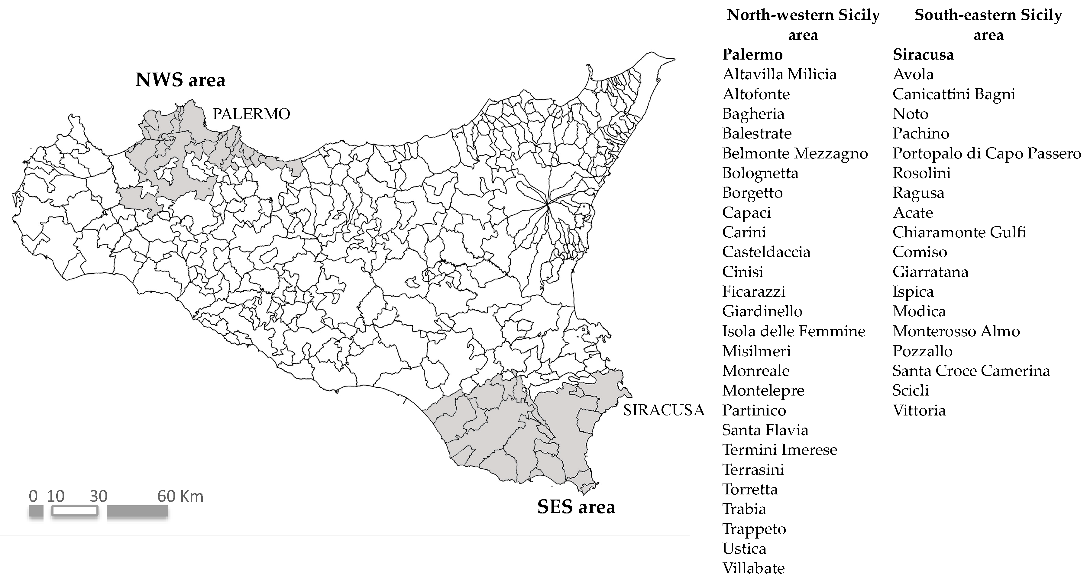
The case study consists of two areas of Sicily (Italy), which are medium-size metropolitan areas located in a less developed European region:, the metropolitan area of Palermo, in north-western Sicily (NWS), and the south-eastern Sicily (SES) area in which the major city is Siracusa (Figure 1). The metropolitan area of Palermo had 1,070,681 inhabitants in 2015 and comprises the city of Palermo (which is the political and administrative capital of the Sicilian Region) and 26 municipalities. The SES area comprises the city of Siracusa, which had 552,766 inhabitants in 2015 and is the capital city of the homonymous province, as well as 18 municipalities.
The two areas are very different. In the former case, the capital city (Palermo) has 674,435 inhabitants, corresponding to 63% of the entire population of the metropolitan area; it is, therefore, a polarised and hierarchical region, where small towns gravitate to the largest city in which the most important administrative, economic, and political functions are located. Palermo nowadays maintains a high attractiveness even if it is reaching a late disurbanisation stage according to the urban lifecycle theory [2,49,50], and a few surrounding towns have begun to form a potential polynuclear city-region [51]. In the latter case, on the other hand, the inhabitants of Siracusa number 122,291, corresponding to just 22.1% of the total SES population. The area includes several medium-size towns (over 50,000 inhabitants), and the territorial structure is closer to a network in which there is not a strong hierarchy, and horizontal relationships between towns are prevalent [52].
4.1. Household Incomes in the Two Metropolitan Areas
From the point of view of wealth creation, expressed by the parameter of gross annual income in 2015 obtained from ISTAT, there are strong differences between the two areas. In fact, the gross annual income produced in the city of Palermo reaches 70.9% of that for the entire NWS area, meaning that it is two and a half times greater than that of the hinterland, and shows that the more profitable economic activities and jobs are located in the capital city. In the SES area, the gross annual income produced in Siracusa is just 28.8% of the total income, which is indicative of the fact that the territorial distribution of wealth is much more even (Figure 2).
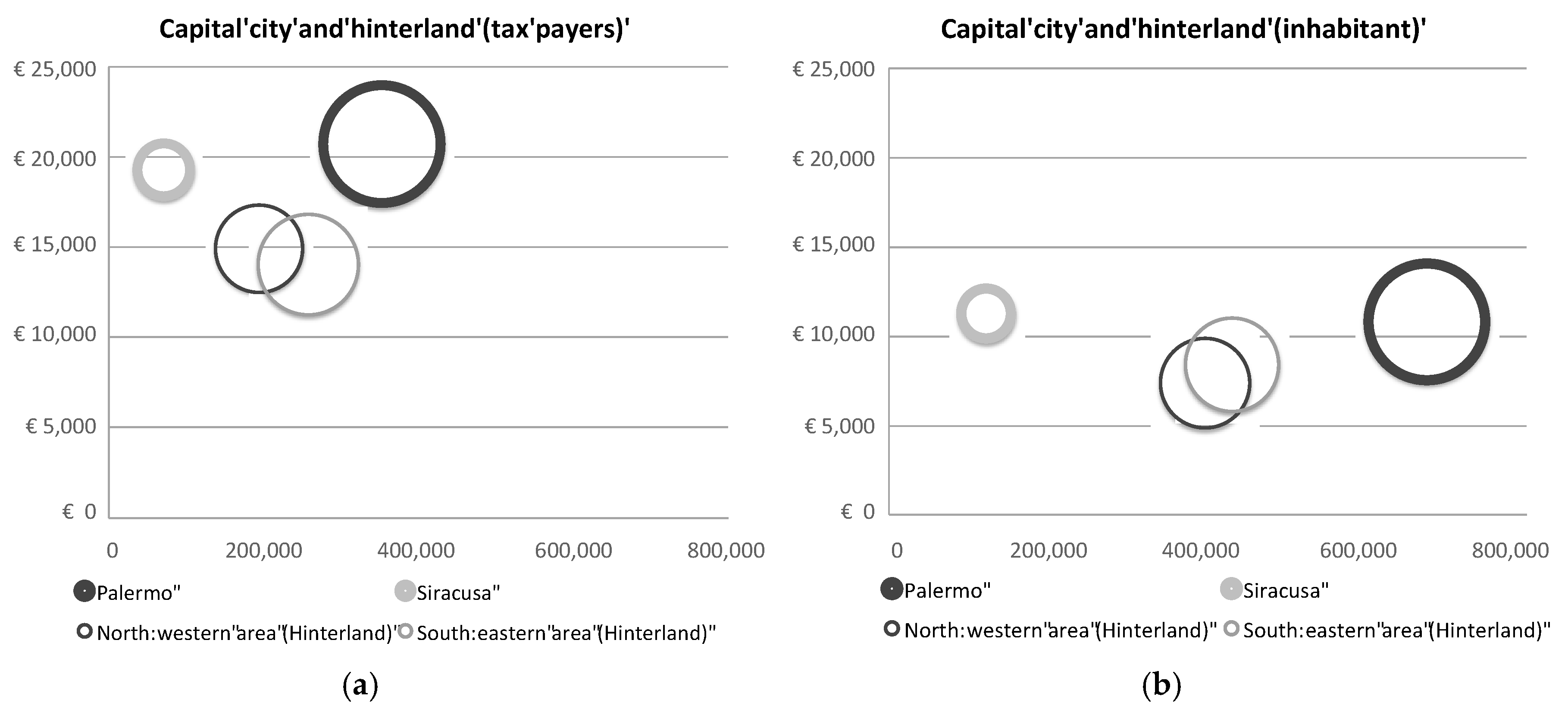
The relationship between the population and the annual average per capita income shows that the income of taxpayers living in the two capital cities is higher than that of those living in the small towns, and this grows as the city rank increases. On the other hand, the annual average per capita incomes of the two hinterlands (each area without a capital city) are very similar, with only a slightly higher average in the area with the smaller hinterland (SES) (Figure 3a). The results are overturned when the annual average per capita income is calculated per inhabitant, and Figure 3b shows that there is a levelling of the incomes: the gross average incomes of the two cities are almost identical and, moreover, are also very close to those of their respective hinterlands. The wealth seems homogeneously distributed within the two metropolitan systems.
The analysis of the annual average per capita income per taxpayer for each municipality of the two hinterlands shows that the income range within the towns in the SES area is wider than that in the NWS area. In the first area, medium-size towns such as Ragusa and Modica (respectively 17,026 and 15,340 euros/year) show both the highest average incomes and the lowest ones (9857 euros/year). In contrast, the annual income range within the metropolitan area in Palermo is smaller, and high average incomes occur even in small towns (e.g., 17,685 euros/year in Isola delle Femmine) (Figure 4a).
The annual average per capita incomes per inhabitant in the hinterlands are all extremely level; the annual income of Ragusa only just exceeds 10,000 euros, confirming, therefore, a homogeneous distribution of the wealth (Figure 4b).
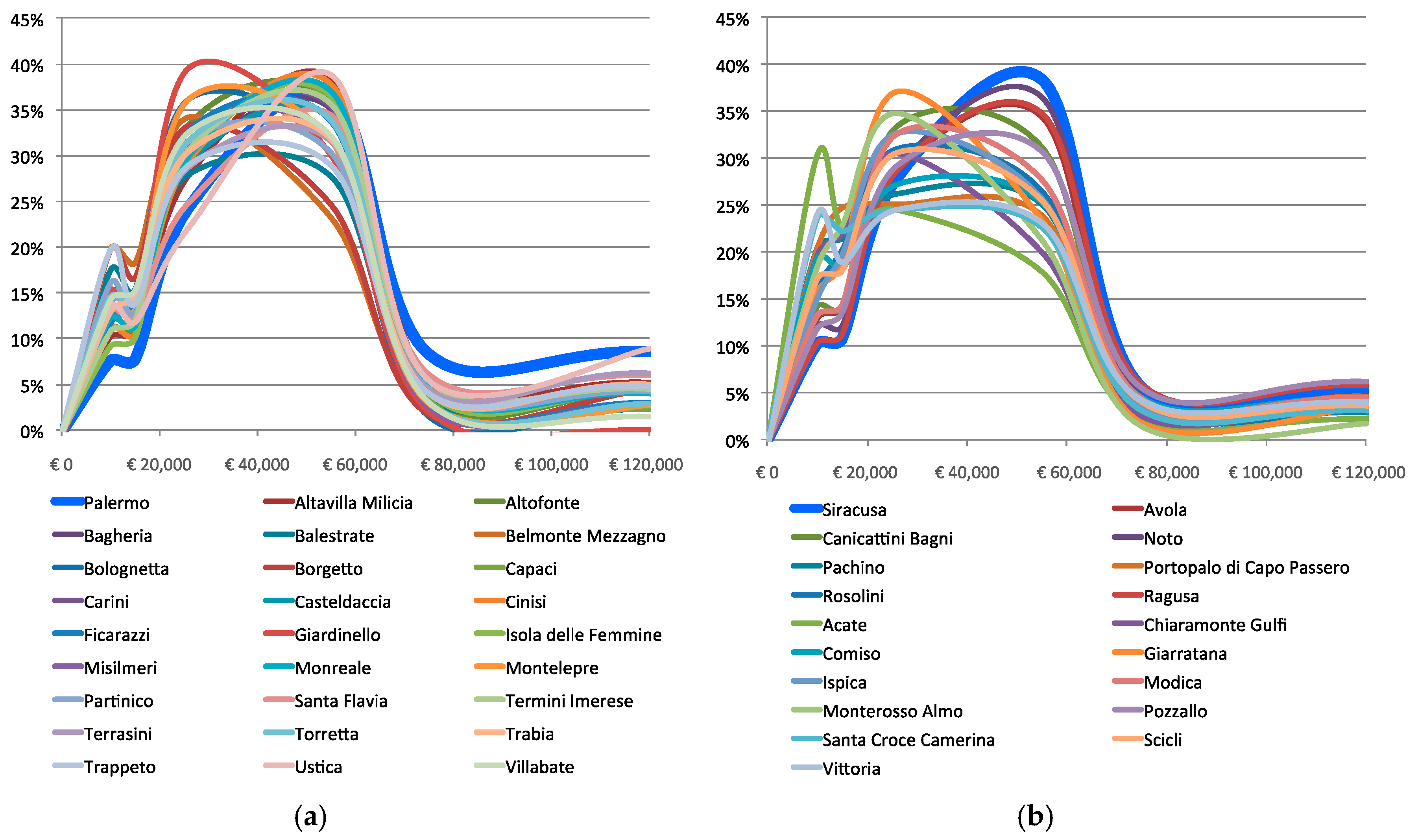
To deepen the study into the territorial distribution of wealth, the analysis of the annual income levels per taxpayer has been made in each municipality, expressing the frequency of each level in percentage terms. The income data derived from ISTAT are broken down by municipality and according to eight levels, which are minor or equal to zero; 0 to 10,000; 10,000 to 15,000; 15,000 to 26,000; 26,000 to 55,000; 55,000 to 75,000; 75,000 to 120,000; and above 120,000 euros/year [53].
Figure 5a shows that the most frequent annual income levels in the NWS area are those in the ranges of 15,000 to 26,000 euros/year and 26,000 to 55,000 euros/year, even if several municipalities have significant percentages (up to 20%) in the lowest income levels, from 0 to 10,000 and from 10,000 to 15,000 euros/year. The highest income levels (75,000 to 120,000 euros/year) register small percentages, and the maximum one (8.6%) occurs in Palermo. In the SES area, on the other hand, the distribution is very diversified (Figure 5b). In many municipalities, the lowest income levels register high percentages of up to 30%, whilst, in a few municipalities, the 15,000 to 26,000 euros/year level registers the highest percentage, and, in other towns, the 26,000 to 55,000 euros/year level is the most common (e.g., Siracusa, Ragusa, and Noto). For all municipalities, the high-income levels have a small percentage, which is less than 5% or absent.
ISTAT calculates the National poverty threshold for a household of a given size and type in Italy [53]. The incomes corresponding to the poverty line are disaggregated by geographical region (northern, central, and southern Italy), by municipality type (centres of metropolitan areas, suburbs of metropolitan areas or towns of more than 50,000 inhabitants, and towns of less than 50,000 inhabitants that are not a part of a metropolitan area), and by household size and type (number of members, ages of adults and children).
The basic poverty line is calculated for two adult households, and, therefore, the coefficients of equivalence are elaborated to convert the basic income into those of different household sizes. ISTAT has also termed households with an income that is up to +20% higher than the poverty line income as ‘nearly poor’.
To test the methodology, a specific household type, comprised of two adults from 18 to 59 years old and one child from four to 10 years old, has been selected. In 2015, the poverty threshold incomes for southern Italy were, respectively, 12,840, 12,516, and 11,952 euros/year for selected households living in the centre of a metropolitan area, in the suburbs of a metropolitan area or a town of more than 50,000 inhabitants, or in a town of less than 50,000 inhabitants that was not part of a metropolitan area.
With regard to Equation (5), the housing cost set by ISTAT has been subtracted from the minimum income of the poverty threshold to obtain the affordable non-housing expenditure for a poor household. The same calculation has also been made for a ‘nearly poor’ household (see Table 1).
4.2. Housing Prices in the Two Metropolitan Areas
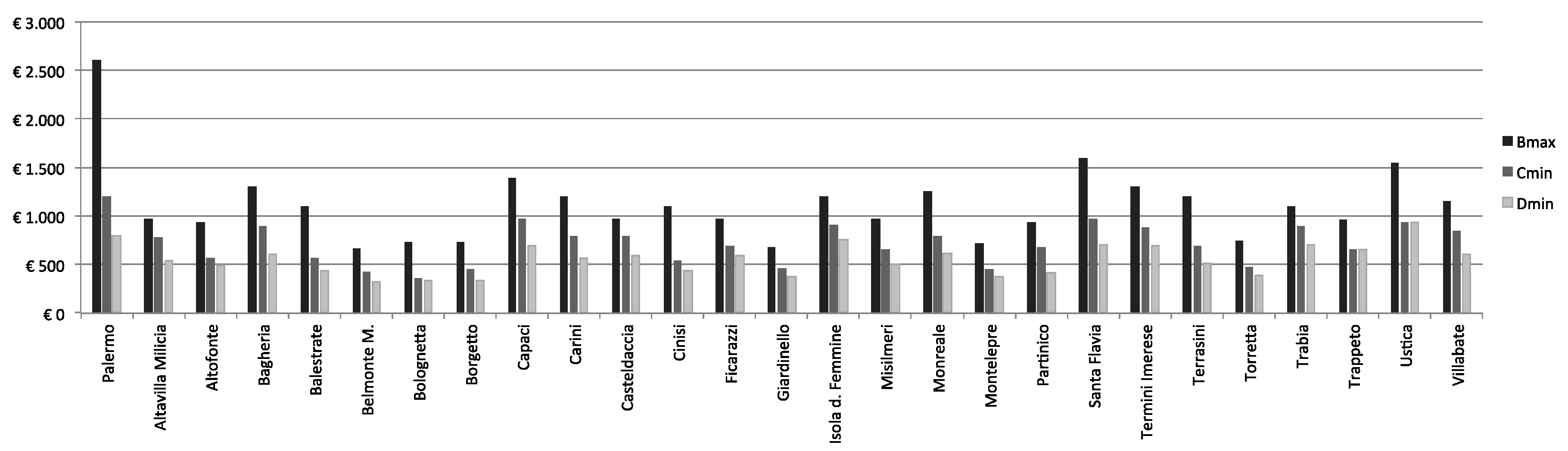
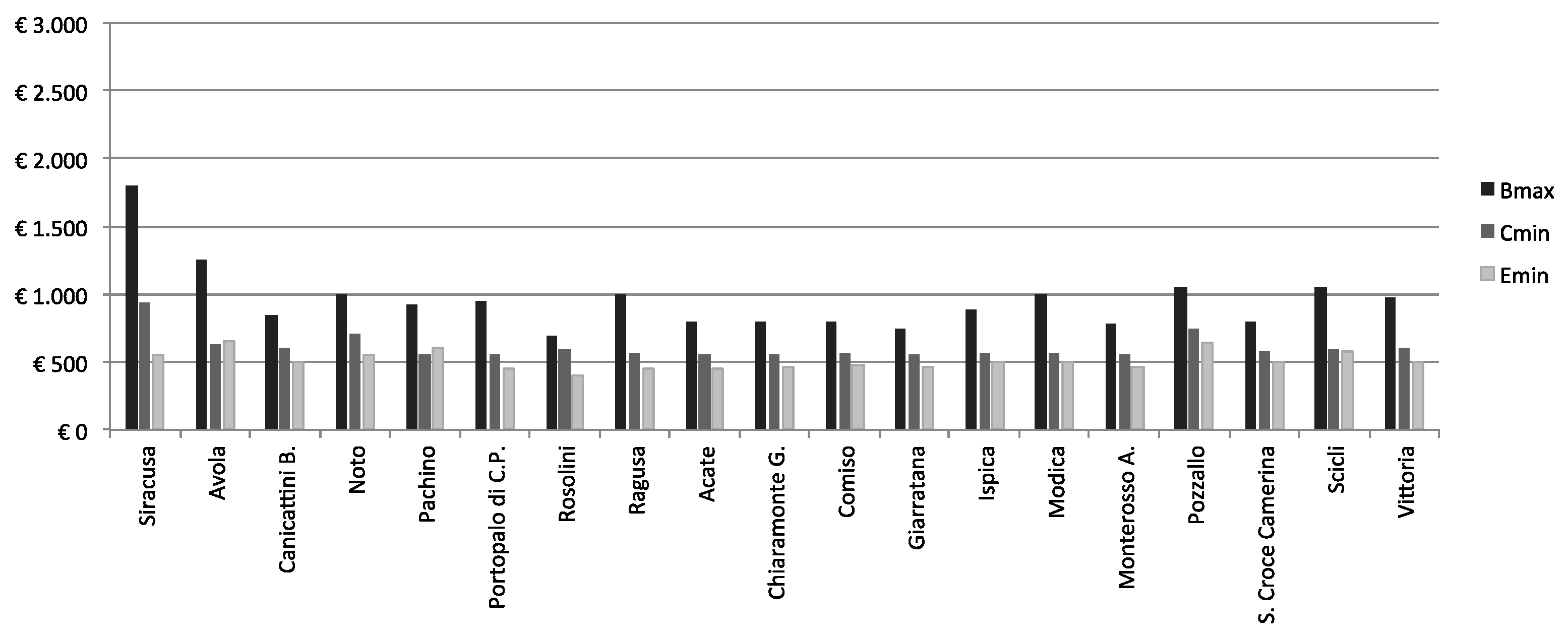
Housing price is a key factor for measuring housing affordability because its spatial distribution expresses the monetary form of the city corresponding to the particular characteristics of each zone (e.g., distance to the city centre, kind and number of amenities, housing quality, etc.). Market prices may be analysed by using several models [54,55,56]. In this study, the housing prices are taken from the OMI database since it is easily accessible and includes housing prices by town and by zone across the Italian territory. The minimum and maximum prices are available per housing type. The housing affordability could be calculated for each price, but, for an analysis at a metropolitan scale, a price range has been selected that may better briefly represent the location in a given town. According to the zone codification by OMI [57], to test the specific affordability in each municipality, the prices for purchasing selected types of housing have been considered to be representative of the local housing market:
- the maximum price Bmax of a housing located in zone B1, which is an inner zone;
- the minimum price Cmin of a housing located in zone C1, which is a middle zone;
- the minimum price Dmin of a housing located in zone D1, which is an outer zone.
In zones B1 and C1, housing standards are respected because the prices refer to mid-range housing, namely ‘civil housing’ by OMI [57], whereas the minimum price in zone D1 is refers to low-range housing, namely ‘cheap housing’, where there may be some deprivation and the quality of housing is low. This latter datum is considered significant to verify the housing affordability, at least for low housing standards and peripheral locations. In the case of the city of Palermo, the selected zones are: B5 as the inner zone; C11 as the middle zone; and E22 as the outer zone.
The data are represented in the Figure 6 and Figure 7 for the NWS and SES areas, respectively. The comparison of the prices within the metropolitan area of Palermo reveals a great differential between the inner zone (zone B5) in the capital city and those in the other towns; the differential depends clearly on Palermo’s high rank. In fact, it also occurs that the housing prices in the outer zones of Palermo are similar to those for the inner zones of the other towns. The minimum price of low-quality housing in zone D1 is very low and ranges from 320 to 940 euros/m2 (Figure 6).
In contrast, the housing prices in the SES area are more homogeneous as a consequence of the regional polynuclear territorial structure. In fact, the differences between the housing prices in the principal city (Siracusa) and those in the other towns are not too pronounced (Figure 7), and the Bmax average price within the hinterland is equal to 50% of the Bmax in Siracusa. The minimum prices of ‘cheap’ housing are 510 euros/m2, and these never rise above 650 euros/m2.
4.3. Calculation of the Threshold-Income in the Metropolitan Areas
The threshold-income has been calculated by applying both the ratio income and the residual income to the housing prices of zones B1, C1, and D1 of each town of the two metropolitan areas, applying Squations 2, 3, 5, and 7 and the parameters in Table 1 and Table 2. Table 3, Table 4 and Table 5 respectively show the calculation of the T_I_ratio, as well as the T_I_residual and the T_I_combined in some towns of the NWS area.
5. Results
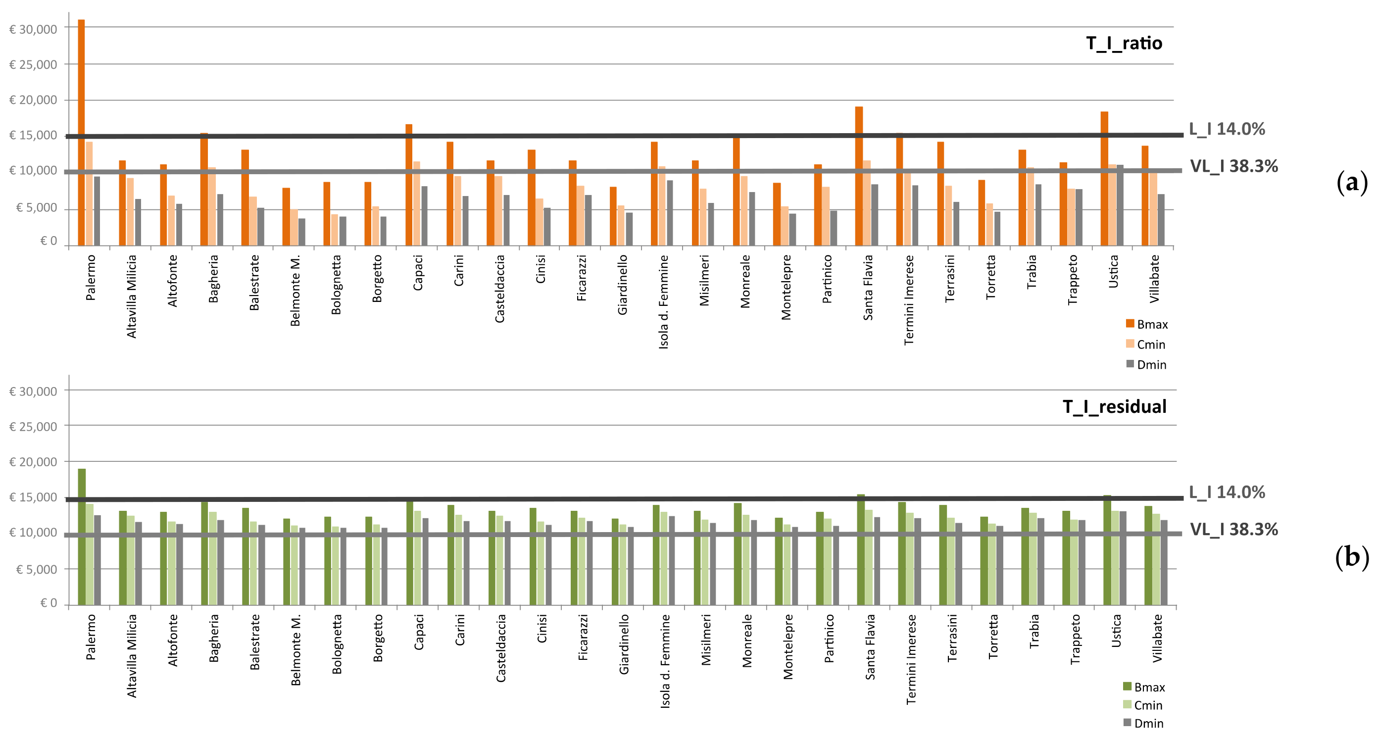
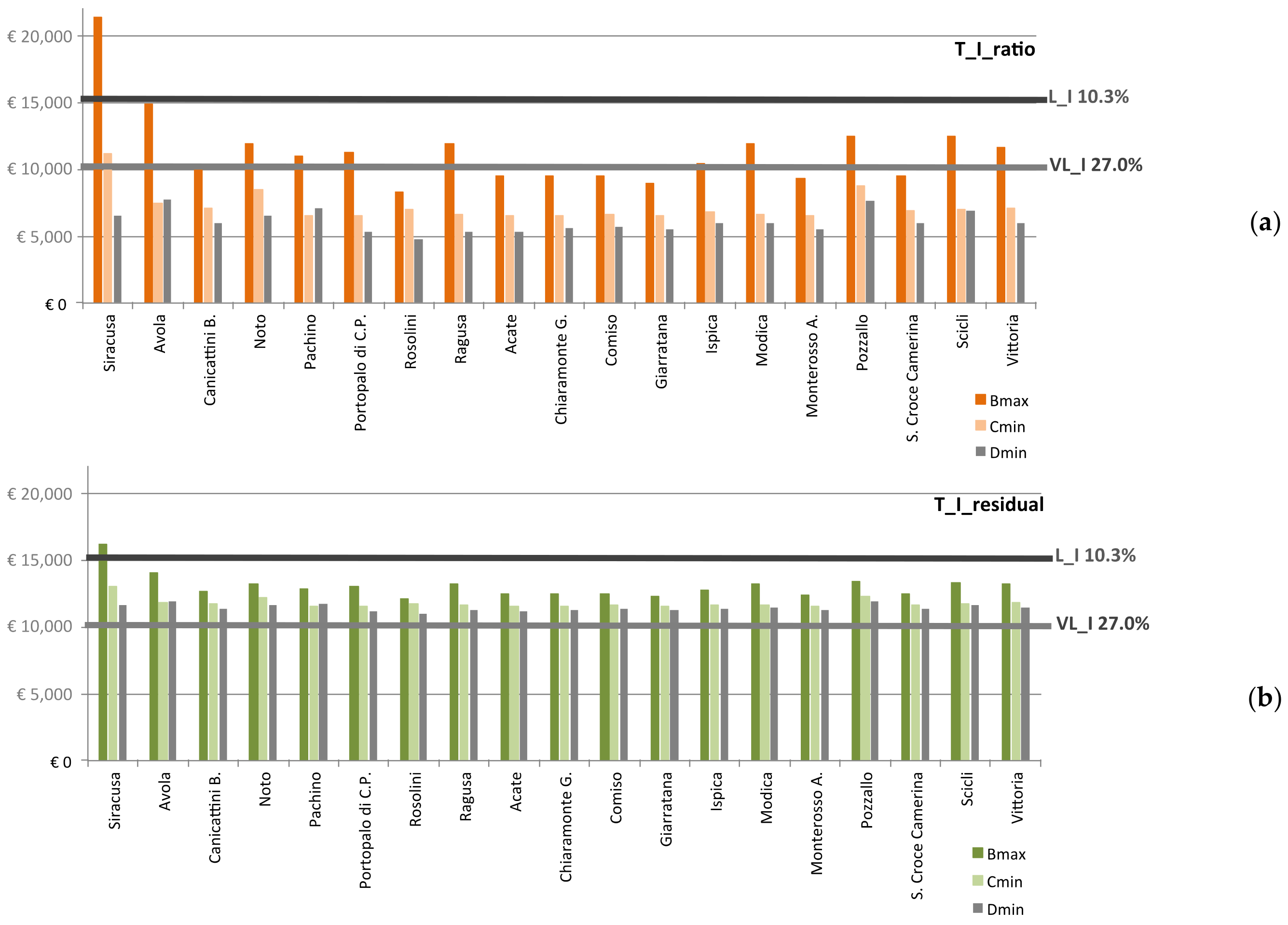
The T_I_ratios and T_I_residuals calculated above are compared, according to the ISTAT income levels, with the very low income (VL_I) level, from 0 to 10,000 euros/year, and with the low income (L_I) level, from 10,000 to 15,000 euros/year, to verify the presence or absence of housing affordability problems in the two metropolitan areas (Figure 8 and Figure 9).
Analysing the potential housing affordability problems of these household types is significant in terms of welfare policy and the actions of social and public housing since they exceed half of the total households in the NWS area, whereas they represent 37.3% of total households in the SES area, indicating that poverty affects a smaller percentage of people in comparison to the former area.
Figure 8 and Figure 9 and Table 6 and Table 7 show that the L_I households have good housing affordability in almost all towns in the two metropolitan areas. They may purchase a house in all the zones, except for the inner zones of the capital cities and of two tourism-oriented towns.
On the other hand, with regard to the resulting T_I_ratio, the central areas of almost all the towns are not affordable for the VL_I households as their income level allows them to purchase housing in the inner zones of the smallest and most marginal towns or a housing of a low standard located in outer zones. The results of the residual income approach profoundly differ from those of the previous approach, as the VL_I is greater than the T_I_residual in none of the zones of any town.
The comparison of the results of the two approaches confirms, in general, that the housing affordability for the VL_I households, which seems real according to the residual income approach, is actually fictitious since the income left is insufficient to meet the minimum needs of the poverty line, even if the housing cost is lower than 30% of the income. On the contrary, the value of the housing affordability is zero, as the results of the residual income approach show, so the VL_I households cannot purchase housing in any zones of any towns in both the NWS and SEA areas.
The similar results for the upper income levels, such as the L_I households, proves that the ratio income approach, although it should be thought of as a ‘rule-of-thumb’, more useful the farther from the poverty line.
The application of the combined income approach provides further results (Table 8):
- the calculation of the residual income approach is confirmed with regard to the VL_I households. There is not housing affordability in any zone of either metropolitan area;
- the housing affordability of the L_I households decreases (i.e., from 24/27 to 17/27 in the NWS area) and is absent in those zones in which the prices are high such as in zone B of the most important towns.
The previous results have two significant implications; one from a methodological point of view, the other from a territorial point of view.
From a methodological point of view, the combined income approach allows us to avoid the most serious distortions in the assessment of housing affordability:
- distortion 1 refers to the ratio income. The same ratio (i.e., 30%) is always used, even if the remaining income is so low that it does not allow the household to cover the non-housing expenditure corresponding to the poverty threshold.
- distortion 2 refers to the residual income. The housing cost is affordable but is too high because it equals a large part of the income, leaving only enough to cover just the minimum non-housing expenditure.
From a methodological point of view, the combined income approach makes it evident that the VL_I households in the metropolitan areas—38.3% in the NWS area and 27% in the SES area—need housing subsidies to locate themselves even in the peripheral zones of small and marginal towns.
The L_I households have, unexpectedly, good housing affordability and may decide to migrate within the metropolitan area and choose to localise in the inner zones of many towns, even if they are excluded from the inner zones of the capital cities and of the most important towns.
6. Concluding Remarks
This study has assessed the housing affordability in two metropolitan areas in a less developed European region with the aim of defining the spatial distribution of the income gap and the affordable zones, which may support metropolitan and urban planning.
The methodology has used a combined income approach, including ratio income and residual income, which was proposed in the literature. This has been applied with a particular emphasis on the analysis of the real estate market, which is considered a key factor. Consequently, the housing prices were collected for each town and urban zone. Nevertheless the ratio income approach has been applied by several national public institutions, and the results confirm its methodological weakness, which can be overcome by using the combined income approach.
The assessment of the combined income in two Sicilian metropolitan areas shows that the fall in prices on the housing market has made the purchase of housing more affordable even for low-income households that live in a marginal European region. On the other hand, very low-income households need housing subsidies, as well as planning able to transform the urban form in order to mitigate social polarization. Public programs or projects are necessary, for example, in the NWA, because its polarized territorial structure has generated high differentials with respect to housing prices. The increase of these differentials tends to exclude very low-income households from the biggest towns or to ghettoize them in a very spatially constrained market on the fringe of the metropolitan area.
The elaboration and representation of the results may be improved in further studies by applying the geographic information system (GIS) system to represent the territorial distribution of income levels and T_I_combined in order to better identify the weakest zones in terms of low-income levels or high market prices. In the assessment of the threshold-incomes, transportation costs could also be included [26] in order to study the potential internal migratory flows within the metropolitan area.
Conflicts of Interest
The author declares no conflicts of interest.
References
- Bruegmann, R. Sprawl: A Compact History; University of Chicago Press: Chicago, IL, USA, 2005. [Google Scholar]
- Van den Berg, L.; Drewett, R.; Klaassen, L.H. Urban Europe: A Study of Growth and Decline; Pergamon: Oxford, UK, 1982. [Google Scholar]
- Soja, E.W. Postmetropolis: Critical Studies of Cities and Regions; Blackwell: Malden, MA, USA, 2000. [Google Scholar]
- Beguin, H. Urban Hierarchy and the Rank-size Distribution. Geogr. Anal. 1979, 11, 149–164. [Google Scholar] [CrossRef]
- Dematteis, G. Contro-urbanizzazione e strutture urbane reticolari. In Sviluppo Multiregionale: Teorie, Metodi, Problem; Bianchi, G., Magnani, I., Eds.; Franco Angeli: Milano, Italy, 1985; pp. 121–132. [Google Scholar]
- Camagni, R. From City-hierarchy to City-network: reflections on Emerging Paradigm. In Structure and Development in the Space Economy: Essays in Honor of Martin Beckmann; Lackshmanan, T.R., Nijkamp, P., Eds.; Springer: Berlin, Germany, 1992; pp. 87–114. [Google Scholar]
- Czamanski, S. A Model of Urban Growth. Pap. Proc. Reg. Sci. Assoc. 1964, 13, 177–200. [Google Scholar] [CrossRef]
- Camagni, R.; Cappellin, R. Struttura economica regionale e integrazione economica europea. Econ. Politica Ind. 1980, 27, 21–76. [Google Scholar]
- Alonso, W. Location and Land Use: Towards a General Theory of the Land Rent; Harvard University Press: Cambridge, UK, 1964. [Google Scholar]
- Fujita, M. Urban Economy Theory: Land Use and City Size; Cambridge University Press: Cambridge, UK, 1989. [Google Scholar]
- Stone, M.E.; Burke, T.; Ralston, L. The Residual Income Approach to Housing Affordability: The Theory and the Practise, 2011. Available online: http://works.bepress.com/michael_stone/7 (accessed on 28 July 2017).
- Heylen, K.; Haffner, M. A ratio or budget benchmark for comparison affordability across countries? J. Hous. Built Environ. 2013, 28, 547–565. [Google Scholar] [CrossRef]
- Hedin, K.; Clark, E.; Lundholm, E.; Malmberg, G. Neoliberalization of housing in Sweden: Gentrification, filtering and social polarization. Ann. Assoc. Am. Geogr. 2012, 102, 443–463. [Google Scholar] [CrossRef]
- Burke, T.; Ralston, L. Measuring housing affordability. AHURI Res. Policy Bull. 2004, 45. Available online: https://www.ahuri.edu.au/research/research-and-policy-bulletins/45 (accessed on 28 July 2017).
- Hancock, K.E. ‘Can pay? Won’t pay?’ or economic principles of affordability. Urban Stud. 1993, 30, 127–145. [Google Scholar] [CrossRef]
- Hulchanski, J.D. The concept of housing affordability: Six contemporary uses of the housing expenditure-to-income. Hous. Stud. 1995, 10, 471–491. [Google Scholar] [CrossRef]
- CDP Cassa Depositi e Prestiti: Report Monografico 03—Social Housing. Il Mercato Immobiliare in Italia: Focus su L’edilia Sociale. 2014. Available online: http://www.cdpisgr.it/static/upload/cdp/cdp-report-monografico_social-housing.pdf (accessed on 28 July 2017).
- Bonafede, G.; Napoli, G. Palermo Multiculturale tra gentrification e crisi del mercato immobiliare nel centro storico. Arch. Stud. Urbani Reg. 2015, 113, 123–150. [Google Scholar] [CrossRef]
- Stone, M.E. A housing affordability standard for the UK. Hous. Stud. 2006, 21, 453–476. [Google Scholar] [CrossRef]
- Rizzo, F. Valori e Valutazioni. La scienza dell’economia o L’economia Della Scienza; FrancoAngeli: Milano, Italy, 1999. [Google Scholar]
- Rizzo, F. Dalla Rivoluzione Keynesiana Alla Nuova Economia. Dis-Equilibrio, Tras-in-Formazione e Coefficiente di Capitalizzazione; FrancoAngeli: Milano, Italy, 2002. [Google Scholar]
- Napoli, G. The Economic Sustainability of Residential Location and Social Housing. An Application in Palermo City. Aestimum 2016, 257–277. Available online: http://www.fupress.net/index.php/ceset/article/view/17896/16729 (accessed on 28 July 2017).
- Napoli, G.; Giuffrida, S.; Trovato, M.R. Fair Planning and Affordability Housing in Urban Policy. The Case of Syracuse (Italy). In Computational Science and Its Applications—ICCSA 2016; Gervasi, O., Murgante, B., Misra, S., Rocha, A.M.A.C., Torre, C.M., Taniar, D., Apduhan, B.O., Stankova, E., Wang, S., Eds.; Springer International Publishing: Cham, Switzerland, 2016; Volume 9789, pp. 46–62. [Google Scholar] [CrossRef]
- Napoli, G.; Schilleci, F. An Application of Analytic Network Process in the Planning Process: The Case of an Urban Transformation in Palermo (Italy). In Computational Science and Its Applications—ICCSA 2014; Murgante, B., Misra, S., Rocha, A.M.A.C., Torre, C.M., Rocha, J.G., Taniar, D., Apduhan, B.O., Gervasi, O., Eds.; Springer International Publishing: Cham, Switzerland, 2014; Volume 8581, pp. 300–314. [Google Scholar] [CrossRef]
- Napoli, G. Financial sustainability and morphogenesis of urban transformation project. In Computational Science and Its Applications—ICCSA 2015; Gervasi, O., Murgante, B., Misra, S., Gavrilova, M.L., Rocha, A.M.A.C., Torre, C.M., Taniar, D., Apduhan, B.O., Eds.; Springer International Publishing: Cham, Switzerland, 2015; Volume 9157, pp. 178–193. [Google Scholar] [CrossRef]
- Brookings Institution. The Affordability Index: A New Tool for Measuring the True Affordability of a Housing Choice. 2006. Available online: https://www.brookings.edu/wp-content/uploads/2016/06/20060127_affindex.pdf (accessed on 7 July 2017).
- National Association of Realtors. NAR: Housing Affordability Index (2005). Available online: http://www.realtor.org (accessed on 7 February 2016).
- OMI: Rapporto Immobiliare 2017. Il Settore Residenziale (2017). Available online: http://www.agenziaentrate.gov.it/wps/content/Nsilib/Nsi/Documentazione/omi/Pubblicazioni/Rapporti+immobiliari+residenziali/ (accessed on 7 July 2017).
- HIA/CBA. Housing Report: A Quarterly Review of Housing Affordability. Available online: https://www.commbank.com.au/about-us/news/media-releases/2003/Commonwealth-Bank-HIA-Housing-Report.pdf (accessed on 7 July 2017).
- Baer, W.C. The evolution of housing indicators and housing standards: Some lessons for the future. Public Policy 1976, 24, 361–393. [Google Scholar]
- Bogdon, A.S.; Can, A. Indicators of local housing affordability: Comparative and spatial approaches. Real Estate Econ. 1997, 25, 43–80. [Google Scholar] [CrossRef]
- Dolbeare, C.N. Housing Grants for the Very Poor; Philadelphia Housing Association: Philadelphia, PA, USA, 1966.
- Frieden, B.J. Improving federal housing subsidies: Summary report. In US Congress, House Committee on Banking and Currency. Papers Submitted to Subcommittee on Housing Panels; 92nd Congress, First Session; U.S. Government Publishing Office: Washington, DC, USA, 1971; pp. 473–488. [Google Scholar]
- Newman, D.K. Housing the poor and the shelter to income ratio. In US Congress, House Committee on Banking and Currency. Papers Submitted to Subcommittee on Housing Panels; 92nd Congress, First Session; U.S. Government Publishing Office: Washington, DC, USA, 1971; pp. 555–578. [Google Scholar]
- Lowry, I.S. Housing assistance for low income urban families: A fresh approach. In US Congress, House Committee on Banking and Currency. Papers Submitted to Subcommittee on Housing Panels; 92nd Congress, First Session; U.S. Government Publishing Office: Washington, DC, USA, 1971; pp. 489–523. [Google Scholar]
- Thalmann, P. House poor’ or simply ‘poor’? J. Hous. Econ. 2003, 12, 291–317. [Google Scholar] [CrossRef]
- Pelletiere, D. Getting to the Heart of Housing’s Fundamental Question: How Much Can a Family Afford? NLIHC: Washington, DC, USA, 2008. [Google Scholar]
- Stone, M.E. Shelter Poverty: New Ideas on Housing Affordability; Temple University Press: Philadelphia, PA, USA, 1993. [Google Scholar]
- Feins, J.D.; Lane, T.S. How Much for Housing? Abt Books: Cambridge, MA, USA, 1981. [Google Scholar]
- Haffner, M.; Boumeester, H. The Affordability of Housing in the Netherlands: An Increasing Income Gap between Renting and Owning? Hous. Stud. 2010, 25, 799–820. [Google Scholar] [CrossRef]
- Borrowman, L.; Kazakevitch, G.; Frost, L. What Types of Australian Households are in Housing Affordability Stress? Econ. Pap. 2015, 34, 1–10. [Google Scholar] [CrossRef]
- Mah, J. Can Inclusionary Zoning Help Address the Shortage of Affordable Housing in Toronto? Canadian Policy Research Networks: Ottawa, ON, Canada, 2009; Available online: http://inclusionaryhousing.ca/wp-content/uploads/sites/2/2009/12/Mah-Can-IZ-Help-2009.pdf (accessed on 7 July 2017).
- Gabrielli, L.; Giuffrida, S.; Trovato, M.R. Gaps and Overlaps of Urban Housing Sub-market: Hard Clustering and Fuzzy Clustering Approaches. In Appraisal: From Theory to Practice; Stanghellini, S., Morano, P., Bottero, M., Oppio, A., Eds.; Springer International Publishing: Cham, Switzerland, 2017; pp. 203–219. [Google Scholar]
- Giuffrida, S.; Ventura, V.; Trovato, M.R.; Napoli, G. Axiology of the historical city and the cap rate. The case of the old town of Ragusa Superiore. Valori e Valutazioni 2017, 18, 41–55. [Google Scholar]
- Napoli, G.; Giuffrida, S.; Valenti, A. Forms and functions of the real estate market of Palermo. Science and knowledge in the cluster analysis approach. In Appraisal: From Theory to Practice; Stanghellini, S., Morano, P., Bottero, M., Oppio, A., Eds.; Springer International Publishing: Cham, Switzerland, 2017; pp. 191–202. [Google Scholar]
- Gabrielli, L.; Giuffrida, S.; Trovato, M.R. Functions and Perspective of Public Real Estate in the urban Policies: the Sustainable Development Plan of Syracuse. In Computational Science and Its Applications; Gervasi, O., Murgante, B., Misra, S., Rocha, A.M.A.C., Torre, C.M., Taniar, D., Apduhan, B.O., Stankova, E., Wang, S., Eds.; Springer International Publishing: Cham, Switzerland, 2016; Volume 9789, pp. 13–28. [Google Scholar] [CrossRef]
- Giuffrida, S.; Napoli, G.; Trovato, M.R. Industrial Areas and the City. Equalization and Compensation in a Value-Oriented Allocation Pattern. In Computational Science and Its Applications; Gervasi, O., Murgante, B., Misra, S., Rocha, A.M.A.C., Torre, C.M., Taniar, D., Apduhan, B.O., Stankova, E., Wang, S., Eds.; Springer International Publishing: Cham, Switzerland, 2016; Volume 9789, pp. 79–89. [Google Scholar] [CrossRef]
- Stone, M.E. What is housing affordability? The case for the residual income approach. Hous. Policy Debate 2006, 17, 151–184. [Google Scholar] [CrossRef]
- Picone, M. II ciclo di vita urbana in Sicilia. Riv. Geogr. Ital. 2006, 113, 129–146. [Google Scholar]
- Lo Piccolo, F.; Picone, M.; Schilleci, F. Forme di territori post metropolitan siciliani. Planum J. Urban. 2013, 27, 46–51. [Google Scholar]
- Lotta, F.; Picone, M.; Schilleci, F. An incomplete post-metropolitan area. In Post-Metropolitan Territories. Looking for a New Urbanity; Balducci, A., Fedeli, V., Curci, F., Eds.; Routledge: New York, NY, USA, 2017; pp. 161–182. [Google Scholar]
- Lo Piccolo, F.; Picone, M.; Todaro, V. South-eastern Sicily: A counterfactual post-metropolis. In Post-Metropolitan Territories. Looking for a New Urbanity; Balducci, A., Fedeli, V., Curci, F., Eds.; Routledge: New York, NY, USA, 2017; pp. 183–204. [Google Scholar]
- ISTAT. Report La Povertà in Italia. 2015. Available online: https://www.istat.it/it/archivio/202338 (accessed on 7 July 2017).
- Del Giudice, V.; De Paola, P.; Forte, F. Using Genetic Algorithms for Real Estate Appraisal. Buildings 2017, 7, 31. [Google Scholar] [CrossRef]
- Del Giudice, V.; De Paola, P.; Forte, F. Bayesian neural network models in the appraisal of real estate properties. In Computational Science and Its Applications; Borruso, G., Cuzzocrea, A., Apduhan, B.O., Rocha, A.M.A.C., Taniar, D., Misra, S., Gervasi, O., Torre, C.M., Stankova, E., Murgante, B., Eds.; Springer International Publishing: Cham, Switzerland, 2017; Volume 10406, pp. 478–489. [Google Scholar] [CrossRef]
- Del Giudice, V.; De Paola, P. Spatial analysis of residential real estate rental market with geoadditive models. Stud. Syst. Decis. Control 2017, 86, 155–162. [Google Scholar]
- OMI. Banche dati OMI. Available online: http://www.agenziaentrate.gov.it/wps/content/Nsilib/Nsi/Documentazione/omi/ (accessed on 7 July 2017).
Figure 1.
Geographical location of the north-western Sicily (NWS) and south-eastern Sicily (SES) areas in Italy.
Figure 1.
Geographical location of the north-western Sicily (NWS) and south-eastern Sicily (SES) areas in Italy.

Figure 2.
Gross annual income (2015) per municipality and per metropolitan area for (a) NWS and (b) SES (our elaboration on Italian National Statistical Institute (ISTAT) data).
Figure 2.
Gross annual income (2015) per municipality and per metropolitan area for (a) NWS and (b) SES (our elaboration on Italian National Statistical Institute (ISTAT) data).
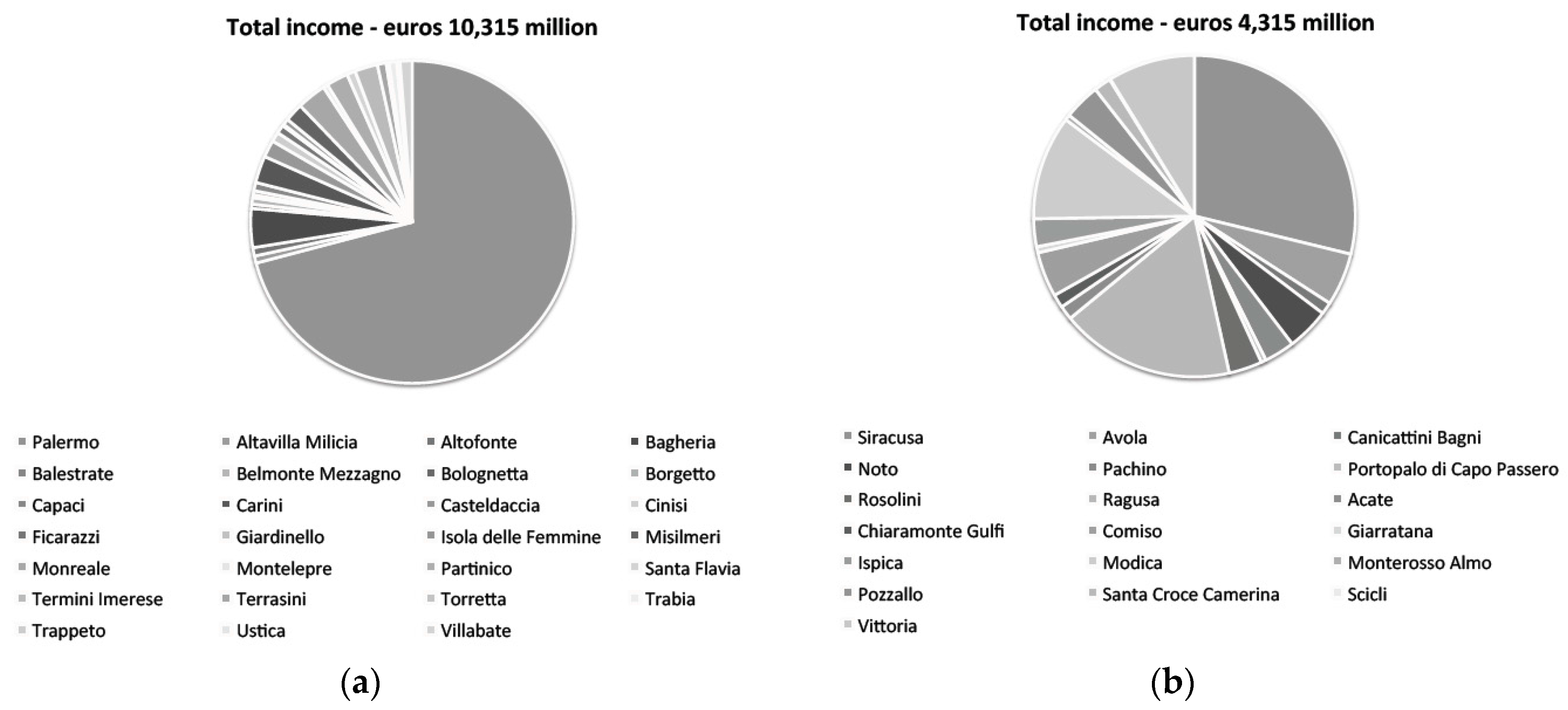
Figure 3.
Population (x-axis) and annual average per capita income (y-axis) of (a) the taxpayers and (b) the inhabitants of the capital cities and their hinterlands (our elaboration on ISTAT data).
Figure 3.
Population (x-axis) and annual average per capita income (y-axis) of (a) the taxpayers and (b) the inhabitants of the capital cities and their hinterlands (our elaboration on ISTAT data).

Figure 4.
Population (x-axis) and average per capita income (y-axis) of (a) the taxpayers and (b) the inhabitants of each town of the hinterland (our elaboration on ISTAT data).
Figure 4.
Population (x-axis) and average per capita income (y-axis) of (a) the taxpayers and (b) the inhabitants of each town of the hinterland (our elaboration on ISTAT data).
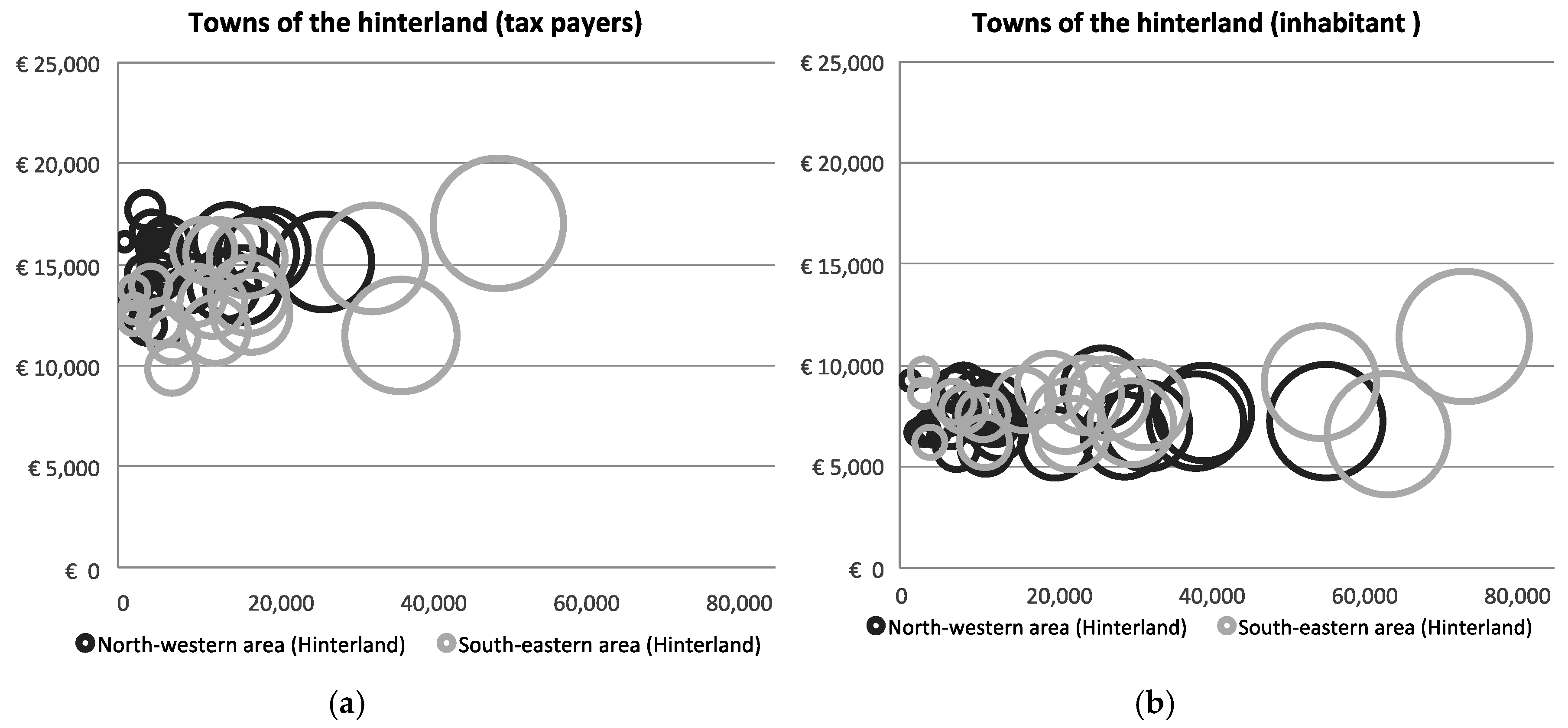
Figure 5.
Percentage of the annual income levels (x-axis) per municipality in the NWS (a) and SES (b) areas (including capital cities) (our elaboration on ISTAT data).
Figure 5.
Percentage of the annual income levels (x-axis) per municipality in the NWS (a) and SES (b) areas (including capital cities) (our elaboration on ISTAT data).

Figure 6.
Purchase. Housing prices in euros/m2 (y-axis) in the municipalities of the NWA area (II semester 2016) (our elaboration on OMI data).
Figure 6.
Purchase. Housing prices in euros/m2 (y-axis) in the municipalities of the NWA area (II semester 2016) (our elaboration on OMI data).

Figure 7.
Purchase. Housing prices in euros/m2 (y-axis) in the municipalities of the SES area (II semester 2016) (our elaboration on Real Estate Market (OMI) data).
Figure 7.
Purchase. Housing prices in euros/m2 (y-axis) in the municipalities of the SES area (II semester 2016) (our elaboration on Real Estate Market (OMI) data).

Figure 8.
T_I_ratio (a) and T_I_residual (b) in euros/year (y-axis) per zone and per municipality of the metropolitan area of Palermo (NWS area).
Figure 8.
T_I_ratio (a) and T_I_residual (b) in euros/year (y-axis) per zone and per municipality of the metropolitan area of Palermo (NWS area).

Figure 9.
T_I_ratio (a) and T_I_residual (b) in euros/year (y-axis) per zone and per municipality in the SES area.
Figure 9.
T_I_ratio (a) and T_I_residual (b) in euros/year (y-axis) per zone and per municipality in the SES area.


Table 1.
Poverty threshold and non-housing expenditure of a family of two adults (from 18 to 59 years old) and one child (from four to 10 years old) in 2015 (our elaboration on ISTAT data).
Table 1.
Poverty threshold and non-housing expenditure of a family of two adults (from 18 to 59 years old) and one child (from four to 10 years old) in 2015 (our elaboration on ISTAT data).
| Town Size | Poverty Income | Non-Housing Expenditure | ||
|---|---|---|---|---|
| Poverty Income | Nearly Poverty Income | |||
| euros/month | euros/year | euros/year | euros/year | |
| Centre of metropolis | €1,070 | €12,840 | €9,713 | €11,656 |
| Metropolitan suburbs and municipalities > 50,000 inhabitants | €1,043 | €12,516 | €9,673 | €11,608 |
| Municipalities < 50,000 inhabitants | €996 | €11,952 | €9,594 | €11,513 |
Table 2.
Parameters for the T_I_ratio calculations
| Parameters | Unit | Value |
|---|---|---|
| Housing size | sqm | 70 |
| Down payment | % | 20 |
| Loan To Value | % | 80 |
| Loan term | years | 20 |
| Annual mortgage rate | % | 2.54 |
| Monthly mortage rate | % | 0.21167 |
| Monthly P&I number | n | 240 |
| Ratio income | % | 30 |
Table 3.
Calculation of the T_I_ratio in some towns of the NWS area (other data omitted).
| Town | Zone | Housing Price | Down Payment | Mortgage | Monthly P&I | T_I_Ratio | ||
|---|---|---|---|---|---|---|---|---|
| Euros/m2 | Euros | Euros | Euros | Euros/Month | Euros/Month | Euros/Year | ||
| Palermo | Bmax | 2600 | 182,000 | 36,400 | 145,600 | 773 | 2576 | 30,910 |
| Palermo | Cmin | 1200 | 84,000 | 16,800 | 67,200 | 357 | 1189 | 14,266 |
| Palermo | Emin | 800 | 56,000 | 11,200 | 44,800 | 238 | 793 | 9511 |
| Altavilla Milicia | Bmax | 980 | 68,600 | 13,720 | 54,880 | 291 | 971 | 11,651 |
| Altavilla Milicia | Cmin | 780 | 54,600 | 10,920 | 43,680 | 232 | 773 | 9273 |
| Altavilla Milicia | Dmin | 540 | 37,800 | 7560 | 30,240 | 160 | 535 | 6420 |
| Altofonte | Bmax | 930 | 65,100 | 13,020 | 52,080 | 276 | 921 | 11,056 |
| Altofonte | Cmin | 570 | 39,900 | 7980 | 31,920 | 169 | 565 | 6776 |
| Altofonte | Dmin | 490 | 34,300 | 6860 | 27,440 | 146 | 485 | 5825 |
| Bagheria | Bmax | 1300 | 91,000 | 18,200 | 72,800 | 386 | 1288 | 15,455 |
| Bagheria | Cmin | 900 | 63,000 | 12,600 | 50,400 | 267 | 892 | 10,700 |
| Bagheria | Dmin | 600 | 42,000 | 8400 | 33,600 | 178 | 594 | 7133 |
| Balestrate | Bmax | 1100 | 77,000 | 15,400 | 61,600 | 327 | 1090 | 13,077 |
| Balestrate | Cmin | 560 | 39,200 | 7840 | 31,360 | 166 | 555 | 6657 |
| Balestrate | Dmin | 440 | 30,800 | 6160 | 24,640 | 131 | 436 | 5231 |
| Belmonte M. | Bmax | 670 | 46,900 | 9380 | 37,520 | 199 | 664 | 7965 |
| Belmonte M. | Cmin | 420 | 29,400 | 5880 | 23,520 | 125 | 416 | 4993 |
| Belmonte M. | Dmin | 320 | 22,400 | 4480 | 17,920 | 95 | 317 | 3804 |
| Bolognetta | Bmax | 730 | 51,100 | 10,220 | 40,880 | 217 | 723 | 8679 |
| Bolognetta | Cmin | 360 | 25,200 | 5040 | 20,160 | 107 | 357 | 4280 |
| Bolognetta | Dmin | 340 | 23,800 | 4760 | 19,040 | 101 | 337 | 4042 |
| Borgetto | Bmax | 730 | 51,100 | 10,220 | 40,880 | 217 | 723 | 8679 |
| Borgetto | Cmin | 450 | 31,500 | 6300 | 25,200 | 134 | 446 | 5350 |
| Borgetto | Dmin | 340 | 23,800 | 4760 | 19,040 | 101 | 337 | 4042 |
| Capaci | Bmax | 1400 | 98,000 | 19,600 | 78,400 | 416 | 1387 | 16,644 |
| Capaci | Cmin | 970 | 67,900 | 13,580 | 54,320 | 288 | 961 | 11,532 |
| Capaci | Dmin | 690 | 48,300 | 9660 | 38,640 | 205 | 684 | 8203 |
Table 4.
Calculation of the T_I_residual in some towns of the NWS area (other data omitted).
| Town | Zone | Monthly P&I | Non-Housing Expenditure | T_I_Residual | |
|---|---|---|---|---|---|
| Euros/Month | Euros/Month | Euros/Month | Euros/Year | ||
| Palermo | Bmax | 773 | 809 | 1582 | 18,985 |
| Palermo | Cmin | 357 | 809 | 1166 | 13,992 |
| Palermo | Emin | 238 | 809 | 1047 | 12,566 |
| Altavilla Milicia | Bmax | 291 | 800 | 1091 | 13,089 |
| Altavilla Milicia | Cmin | 232 | 800 | 1031 | 12,376 |
| Altavilla Milicia | Dmin | 160 | 800 | 960 | 11,520 |
| Altofonte | Bmax | 276 | 800 | 1076 | 12,911 |
| Altofonte | Cmin | 169 | 800 | 969 | 11,627 |
| Altofonte | Dmin | 146 | 800 | 945 | 11,342 |
| Bagheria | Bmax | 386 | 806 | 1192 | 14,310 |
| Bagheria | Cmin | 267 | 806 | 1074 | 12,883 |
| Bagheria | Dmin | 178 | 806 | 984 | 11,813 |
| Balestrate | Bmax | 327 | 800 | 1126 | 13,517 |
| Balestrate | Cmin | 166 | 800 | 966 | 11,591 |
| Balestrate | Dmin | 131 | 800 | 930 | 11,164 |
| Belmonte M. | Bmax | 199 | 800 | 999 | 11,984 |
| Belmonte M. | Cmin | 125 | 800 | 924 | 11,092 |
| Belmonte M. | Dmin | 95 | 800 | 895 | 10,736 |
| Bolognetta | Bmax | 217 | 800 | 1016 | 12,198 |
| Bolognetta | Cmin | 107 | 800 | 907 | 10,878 |
| Bolognetta | Dmin | 101 | 800 | 901 | 10,807 |
| Borgetto | Bmax | 217 | 800 | 1016 | 12,198 |
| Borgetto | Cmin | 134 | 800 | 933 | 11,199 |
| Borgetto | Dmin | 101 | 800 | 901 | 10,807 |
| Capaci | Bmax | 416 | 806 | 1222 | 14,666 |
| Capaci | Cmin | 288 | 806 | 1094 | 13,133 |
| Capaci | Dmin | 205 | 806 | 1011 | 12,134 |
Table 5.
Calculation of the T_I_combined in some towns of the NWS area (other data omitted).
| Town | Zone | Annual P&I | T_I_Residual | Ratio |
|---|---|---|---|---|
| Euros/Year | Euros/Year | Threshold = 30% | ||
| Palermo | Bmax | 9273 | 18,985 | 49% |
| Palermo | Cmin | 4280 | 13,992 | 31% |
| Palermo | Emin | 2853 | 12,566 | 23% |
| Altavilla Milicia | Bmax | 3495 | 13,089 | 27% |
| Altavilla Milicia | Cmin | 2782 | 12,376 | 22% |
| Altavilla Milicia | Dmin | 1926 | 11,520 | 17% |
| Altofonte | Bmax | 3317 | 12,911 | 26% |
| Altofonte | Cmin | 2033 | 11,627 | 17% |
| Altofonte | Dmin | 1748 | 11,342 | 15% |
| Bagheria | Bmax | 4636 | 14,310 | 32% |
| Bagheria | Cmin | 3210 | 12,883 | 25% |
| Bagheria | Dmin | 2140 | 11,813 | 18% |
| Balestrate | Bmax | 3923 | 13,517 | 29% |
| Balestrate | Cmin | 1997 | 11,591 | 17% |
| Balestrate | Dmin | 1569 | 11,164 | 14% |
| Belmonte M. | Bmax | 2390 | 11,984 | 20% |
| Belmonte M. | Cmin | 1498 | 11,092 | 14% |
| Belmonte M. | Dmin | 1141 | 10,736 | 11% |
| Bolognetta | Bmax | 2604 | 12,198 | 21% |
| Bolognetta | Cmin | 1284 | 10,878 | 12% |
| Bolognetta | Dmin | 1213 | 10,807 | 11% |
| Borgetto | Bmax | 2604 | 12,198 | 21% |
| Borgetto | Cmin | 1605 | 11,199 | 14% |
| Borgetto | Dmin | 1213 | 10,807 | 11% |
| Capaci | Bmax | 4993 | 14,666 | 34% |
| Capaci | Cmin | 3460 | 13,133 | 26% |
| Capaci | Dmin | 2461 | 12,134 | 20% |
Note: The bold numbers highlight cases in which the housing cost is lower than the threshold ratio.
Table 6.
Frequency of housing affordability per income level and per zone in the NWS area.
| Household Income Level | Income Level > T_I_Ratio | Income Level > T_I_Residual | ||||
|---|---|---|---|---|---|---|
| Bmax | Cmin | Dmin | Bmax | Cmin | Dmin | |
| euros/year | No. | No. | No. | No. | No. | No. |
| VL_I (0–10,000) | 5/27 | 18/27 | 27/27 | 0/27 | 0/27 | 0/27 |
| L_I (10,000–15,000) | 22/27 | 27/27 | 27/27 | 24/27 | 27/27 | 27/27 |
Table 7.
Frequency of housing affordability per income level and per zone in the SES area.
| Household Income Level | Income Level > T_I_Ratio | Income Level > T_I_Residual | ||||
|---|---|---|---|---|---|---|
| Bmax | Cmin | Dmin | Bmax | Cmin | Dmin | |
| euros/year | No. | No. | No. | No. | No. | No. |
| VL_I (0–10,000) | 7/19 | 18/19 | 19/19 | 0/19 | 0/19 | 0/19 |
| L_I (10,000–15,000) | 18/19 | 19/19 | 19/19 | 18/19 | 19/19 | 19/19 |
Table 8.
Combined income approach. Frequency of housing affordability per income level and per zone in the NWS and SWS areas.
Table 8.
Combined income approach. Frequency of housing affordability per income level and per zone in the NWS and SWS areas.
| Household Income Level | North-Western Area | South-Eastern Area | ||||
|---|---|---|---|---|---|---|
| Bmax | Cmin | Dmin | Bmax | Cmin | Dmin | |
| euros/year | No. | No. | No. | No. | No. | No. |
| VL_I (0–10,000) | 0/27 | 0/27 | 0/27 | 0/19 | 0/19 | 0/19 |
| L_I (10,000–15,000) | 17/27 | 26/27 | 27/27 | 17/19 | 19/19 | 19/19 |
© 2017 by the author. Licensee MDPI, Basel, Switzerland. This article is an open access article distributed under the terms and conditions of the Creative Commons Attribution (CC BY) license (http://creativecommons.org/licenses/by/4.0/).
Share and Cite
MDPI and ACS Style
Napoli, G. Housing Affordability in Metropolitan Areas. The Application of a Combination of the Ratio Income and Residual Income Approaches to Two Case Studies in Sicily, Italy. Buildings 2017, 7, 95. https://doi.org/10.3390/buildings7040095
AMA Style
Napoli G. Housing Affordability in Metropolitan Areas. The Application of a Combination of the Ratio Income and Residual Income Approaches to Two Case Studies in Sicily, Italy. Buildings. 2017; 7(4):95. https://doi.org/10.3390/buildings7040095
Chicago/Turabian StyleNapoli, Grazia. 2017. "Housing Affordability in Metropolitan Areas. The Application of a Combination of the Ratio Income and Residual Income Approaches to Two Case Studies in Sicily, Italy" Buildings 7, no. 4: 95. https://doi.org/10.3390/buildings7040095
Note that from the first issue of 2016, this journal uses article numbers instead of page numbers. See further details here.